In this post, we demonstrate how Kubeflow on AWS (an AWS-specific distribution of Kubeflow) used with AWS Deep Learning Containers and Amazon Elastic File System (Amazon EFS) simplifies collaboration and provides flexibility in training deep learning models at scale on both Amazon Elastic Kubernetes Service (Amazon EKS) and Amazon SageMaker utilizing a hybrid architecture approach.
Machine learning (ML) development relies on complex and continuously evolving open-source frameworks and toolkits, as well as complex and continuously evolving hardware ecosystems. This poses a challenge when scaling out ML development to a cluster. Containers offer a solution, because they can fully encapsulate not just the training code, but the entire dependency stack down to the hardware libraries. This ensures an ML environment that is consistent and portable, and facilitates reproducibility of the training environment on each individual node of the training cluster.
Kubernetes is a widely adopted system for automating infrastructure deployment, resource scaling, and management of these containerized applications. However, Kubernetes wasn’t built with ML in mind, so it can feel counterintuitive to data scientists due to its heavy reliance on YAML specification files. There isn’t a Jupyter experience, and there aren’t many ML-specific capabilities, such as workflow management and pipelines, and other capabilities that ML experts expect, such as hyperparameter tuning, model hosting, and others. Such capabilities can be built, but Kubernetes wasn’t designed to do this as its primary objective.
The open-source community took notice and developed a layer on top of Kubernetes called Kubeflow. Kubeflow aims to make the deployment of end-to-end ML workflows on Kubernetes simple, portable, and scalable. You can use Kubeflow to deploy best-of-breed open-source systems for ML to diverse infrastructures.
Kubeflow and Kubernetes provides flexibility and control to data scientist teams. However, ensuring high utilization of training clusters running at scale with reduced operational overheads is still challenging.
This post demonstrates how customers who have on-premises restrictions or existing Kubernetes investments can address this challenge by using Amazon EKS and Kubeflow on AWS to implement an ML pipeline for distributed training based on a self-managed approach, and use fully managed SageMaker for a cost-optimized, fully managed, and production-scale training infrastructure. This includes step-by-step implementation of a hybrid distributed training architecture that allows you to choose between the two approaches at runtime, conferring maximum control and flexibility with stringent needs for your deployments. You will see how you can continue using open-source libraries in your deep learning training script and still make it compatible to run on both Kubernetes and SageMaker in a platform agnostic way.
How does Kubeflow on AWS and SageMaker help?
Neural network models built with deep learning frameworks like TensorFlow, PyTorch, MXNet, and others provide much higher accuracy by using significantly larger training datasets, especially in computer vision and natural language processing use cases. However, with large training datasets, it takes longer to train the deep learning models, which ultimately slows down the time to market. If we could scale out a cluster and bring down the model training time from weeks to days or hours, it could have a huge impact on productivity and business velocity.
Amazon EKS helps provision the managed Kubernetes control plane. You can use Amazon EKS to create large-scale training clusters with CPU and GPU instances and use the Kubeflow toolkit to provide ML-friendly, open-source tools and operationalize ML workflows that are portable and scalable using Kubeflow Pipelines to improve your team’s productivity and reduce the time to market.
However, there could be a couple of challenges with this approach:
- Ensuring maximum utilization of a cluster across data science teams. For example, you should provision GPU instances on demand and ensure its high utilization for demanding production-scale tasks such as deep learning training, and use CPU instances for the less demanding tasks such data preprocessing
- Ensuring high availability of heavyweight Kubeflow infrastructure components, including database, storage, and authentication, that are deployed in the Kubernetes cluster worker node. For example, the Kubeflow control plane generates artifacts (such as MySQL instances, pod logs, or MinIO storage) that grow over time and need resizable storage volumes with continuous monitoring capabilities.
- Sharing the training dataset, code, and compute environments between developers, training clusters, and projects is challenging. For example, if you’re working on your own set of libraries and those libraries have strong interdependencies, it gets really hard to share and run the same piece of code between data scientists in the same team. Also, each training run requires you to download the training dataset and build the training image with new code changes.
Kubeflow on AWS helps address these challenges and provides an enterprise-grade semi-managed Kubeflow product. With Kubeflow on AWS, you can replace some Kubeflow control plane services like database, storage, monitoring, and user management with AWS managed services like Amazon Relational Database Service (Amazon RDS), Amazon Simple Storage Service (Amazon S3), Amazon Elastic File System (Amazon EFS), Amazon FSx, Amazon CloudWatch, and Amazon Cognito.
Replacing these Kubeflow components decouples critical parts of the Kubeflow control plane from Kubernetes, providing a secure, scalable, resilient, and cost-optimized design. This approach also frees up storage and compute resources from the EKS data plane, which may be needed by applications such as distributed model training or user notebook servers. Kubeflow on AWS also provides native integration of Jupyter notebooks with Deep Learning Container (DLC) images, which are pre-packaged and preconfigured with AWS optimized deep learning frameworks such as PyTorch and TensorFlow that allow you to start writing your training code right away without dealing with dependency resolutions and framework optimizations. Also, Amazon EFS integration with training clusters and the development environment allows you to share your code and processed training dataset, which avoids building the container image and loading huge datasets after every code change. These integrations with Kubeflow on AWS help you speed up the model building and training time and allow for better collaboration with easier data and code sharing.
Kubeflow on AWS helps build a highly available and robust ML platform. This platform provides flexibility to build and train deep learning models and provides access to many open-source toolkits, insights into logs, and interactive debugging for experimentation. However, achieving maximum utilization of infrastructure resources while training deep learning models on hundreds of GPUs still involves a lot of operational overheads. This could be addressed by using SageMaker, which is a fully managed service designed and optimized for handling performant and cost-optimized training clusters that are only provisioned when requested, scaled as needed, and shut down automatically when jobs complete, thereby providing close to 100% resource utilization. You can integrate SageMaker with Kubeflow Pipelines using managed SageMaker components. This allows you to operationalize ML workflows as part of Kubeflow pipelines, where you can use Kubernetes for local training and SageMaker for product-scale training in a hybrid architecture.
Solution overview
The following architecture describes how we use Kubeflow Pipelines to build and deploy portable and scalable end-to-end ML workflows to conditionally run distributed training on Kubernetes using Kubeflow training or SageMaker based on the runtime parameter.
Kubeflow training is a group of Kubernetes Operators that add to Kubeflow the support for distributed training of ML models using different frameworks like TensorFlow, PyTorch, and others. pytorch-operator is the Kubeflow implementation of the Kubernetes custom resource (PyTorchJob) to run distributed PyTorch training jobs on Kubernetes.
We use the PyTorchJob Launcher component as part of the Kubeflow pipeline to run PyTorch distributed training during the experimentation phase when we need flexibility and access to all the underlying resources for interactive debugging and analysis.
We also use SageMaker components for Kubeflow Pipelines to run our model training at production scale. This allows us to take advantage of powerful SageMaker features such as fully managed services, distributed training jobs with maximum GPU utilization, and cost-effective training through Amazon Elastic Compute Cloud (Amazon EC2) Spot Instances.
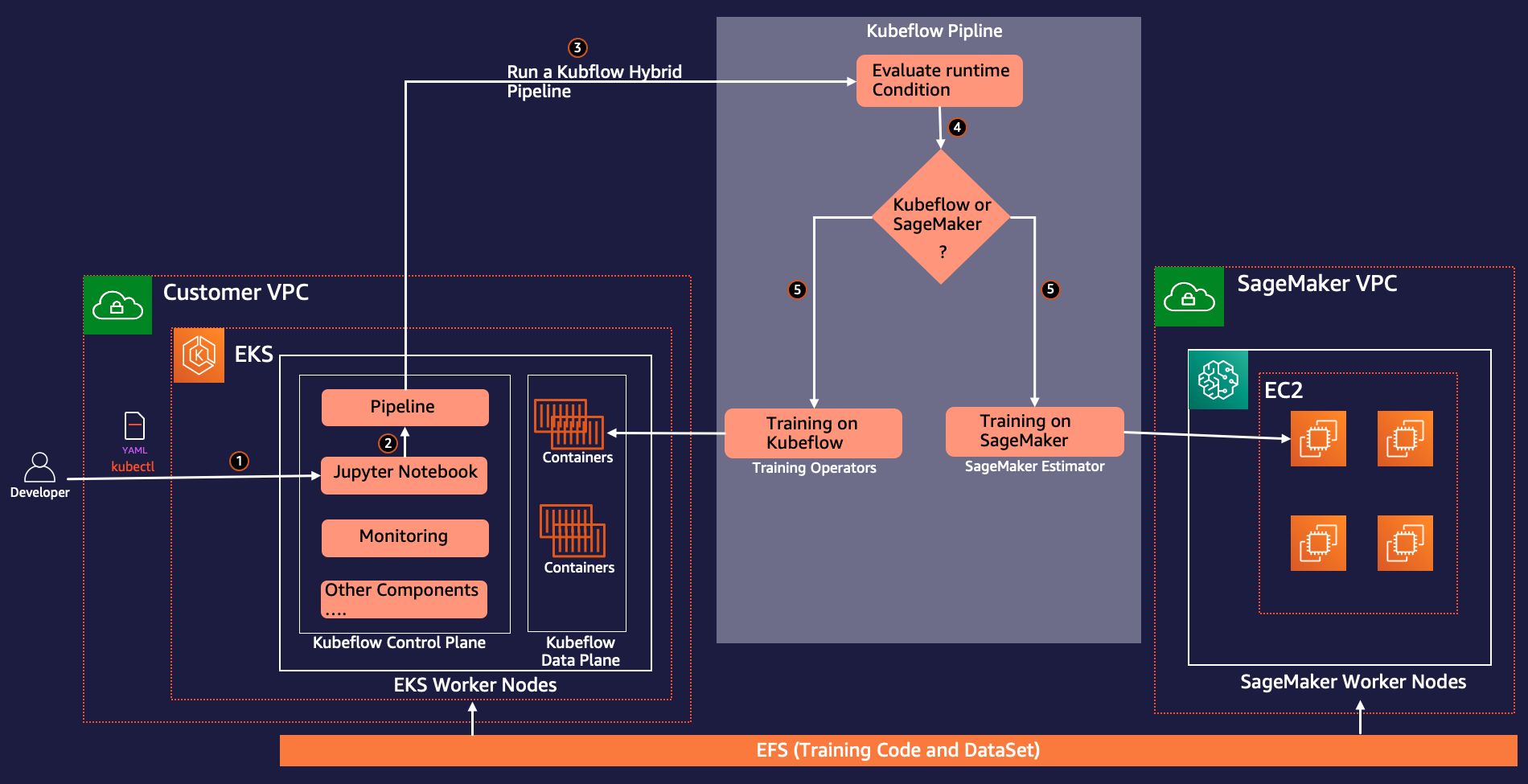
As part for the workflow creation process, you complete the following steps (as shown in the preceding diagram) to create this pipeline:
- Use the Kubeflow manifest file to create a Kubeflow dashboard and access Jupyter notebooks from the Kubeflow central dashboard.
- Use the Kubeflow pipeline SDK to create and compile Kubeflow pipelines using Python code. Pipeline compilation converts the Python function to a workflow resource, which is an Argo-compatible YAML format.
- Use the Kubeflow Pipelines SDK client to call the pipeline service endpoint to run the pipeline.
- The pipeline evaluates the conditional runtime variables and decides between SageMaker or Kubernetes as the target run environment.
- Use the Kubeflow PyTorch Launcher component to run distributed training on the native Kubernetes environment, or use the SageMaker component to submit the training on the SageMaker managed platform.
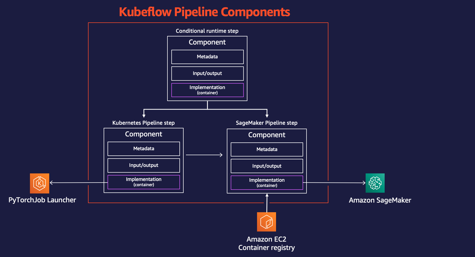
The following figure shows the Kubeflow Pipelines components involved in the architecture that give us the flexibility to choose between Kubernetes or SageMaker distributed environments.
Use Case Workflow
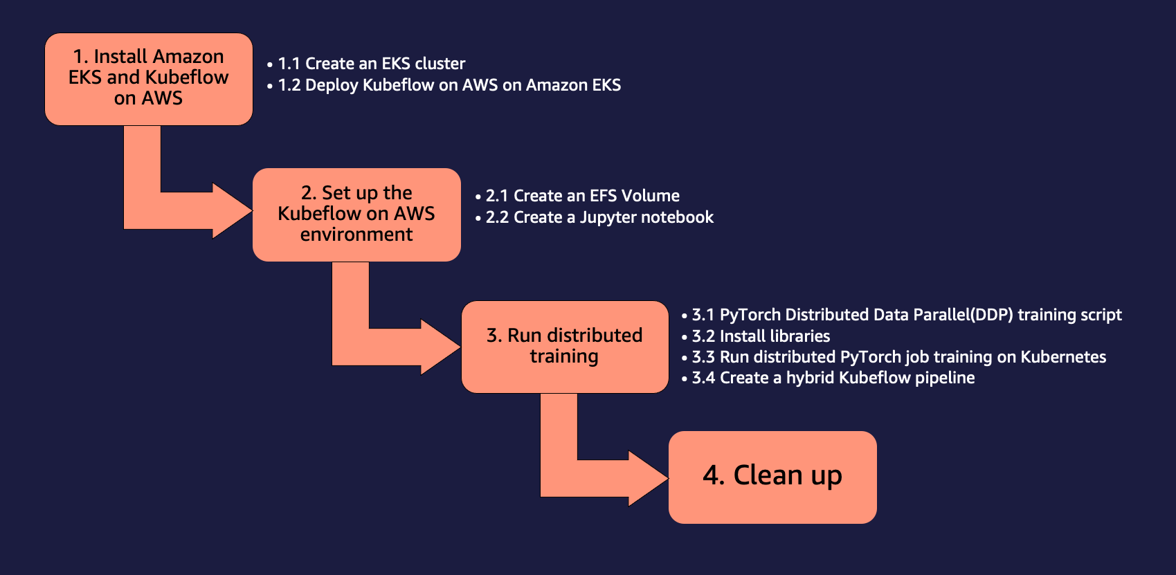
We use the following step-by-step approach to install and run the use case for distributed training using Amazon EKS and SageMaker using Kubeflow on AWS.
Prerequisites
For this walkthrough, you should have the following prerequisites:
- An AWS account.
- A machine with Docker and the AWS Command Line Interface (AWS CLI) installed.
- Optionally, you can use AWS Cloud9, a cloud-based integrated development environment (IDE) that enables completing all the work from your web browser. For setup instructions, refer to Setup Cloud9 IDE. From your Cloud9 environment, choose the plus sign and open new terminal.
-
Create a role with the name
sagemakerrole. Add managed policiesAmazonSageMakerFullAccessandAmazonS3FullAccessto give SageMaker access to S3 buckets. This role is used by SageMaker job submitted as part of Kubeflow Pipelines step. - Make sure your account has SageMaker Training resource type limit for
ml.p3.2xlargeincreased to 2 using Service Quotas Console
1. Install Amazon EKS and Kubeflow on AWS
You can use several different approaches to build a Kubernetes cluster and deploy Kubeflow. In this post, we focus on an approach that we believe brings simplicity to the process. First, we create an EKS cluster, then we deploy Kubeflow on AWS v1.5 on it. For each of these tasks, we use a corresponding open-source project that follows the principles of the Do Framework. Rather than installing a set of prerequisites for each task, we build Docker containers that have all the necessary tools and perform the tasks from within the containers.
We use the Do Framework in this post, which automates the Kubeflow deployment with Amazon EFS as an add-on. For the official Kubeflow on AWS deployment options for production deployments, refer to Deployment.
Configure the current working directory and AWS CLI
We configure a working directory so we can refer to it as the starting point for the steps that follow:
We also configure an AWS CLI profile. To do so, you need an access key ID and secret access key of an AWS Identity and Access Management (IAM) user account with administrative privileges (attach the existing managed policy) and programmatic access. See the following code:
1.1 Create an EKS cluster
If you already have an EKS cluster available, you can skip to the next section. For this post, we use the aws-do-eks project to create our cluster.
- First clone the project in your working directory
- Then build and run the
aws-do-ekscontainer:The
build.shscript creates a Docker container image that has all the necessary tools and scripts for provisioning and operation of EKS clusters. Therun.shscript starts a container using the created Docker image and keeps it up, so we can use it as our EKS management environment. To see the status of youraws-do-ekscontainer, you can run./status.sh. If the container is in Exited status, you can use the./start.shscript to bring the container up, or to restart the container, you can run./stop.shfollowed by./run.sh. - Open a shell in the running
aws-do-ekscontainer: - To review the EKS cluster configuration for our KubeFlow deployment, run the following command:
By default, this configuration creates a cluster named
eks-kubeflowin theus-west-2Region with six m5.xlarge nodes. Also, EBS volumes encryption is not enabled by default. You can enable it by adding"volumeEncrypted: true"to the nodegroup and it will encrypt using the default key. Modify other configurations settings if needed. - To create the cluster, run the following command:
The cluster provisioning process may take up to 30 minutes.
- To verify that the cluster was created successfully, run the following command:
The output from the preceding command for a cluster that was created successfully looks like the following code:
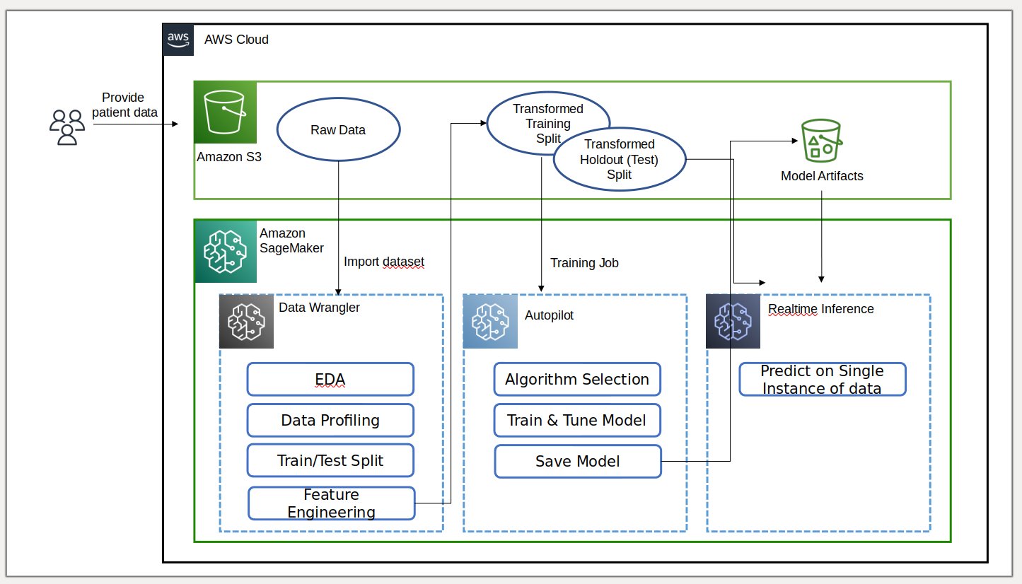
Create an EFS volume for the SageMaker training job
In this use case, you speed up the SageMaker training job by training deep learning models from data already stored in Amazon EFS. This choice has the benefit of directly launching your training jobs from the data in Amazon EFS with no data movement required, resulting in faster training start times.
We create an EFS volume and deploy the EFS Container Storage Interface (CSI) driver. This is accomplished by a deployment script located in /eks/deployment/csi/efs within the aws-do-eks container.
This script assumes you have one EKS cluster in your account. Set CLUSTER_NAME=<eks_cluster_name> in case you have more than one EKS cluster.
This script provisions an EFS volume and creates mount targets for the subnets of the cluster VPC. It then deploys the EFS CSI driver and creates the efs-sc storage class and efs-pv persistent volume in the EKS cluster.
Upon successful completion of the script, you should see output like the following:
Create an Amazon S3 VPC endpoint
You use a private VPC that your SageMaker training job and EFS file system have access to. To give the SageMaker training cluster access to the S3 buckets from your private VPC, you create a VPC endpoint:
You may now exit the aws-do-eks container shell and proceed to the next section:
1.2 Deploy Kubeflow on AWS on Amazon EKS
To deploy Kubeflow on Amazon EKS, we use the aws-do-kubeflow project.
- Clone the repository using the following commands:
- Then configure the project:
This script opens the project configuration file in a text editor. It’s important for AWS_REGION to be set to the Region your cluster is in, as well as AWS_CLUSTER_NAME to match the name of the cluster that you created earlier. By default, your configuration is already properly set, so if you don’t need to make any changes, just close the editor.
The
build.shscript creates a Docker container image that has all the tools necessary to deploy and manage Kubeflow on an existing Kubernetes cluster. Therun.shscript starts a container, using the Docker image, and the exec.sh script opens a command shell into the container, which we can use as our Kubeflow management environment. You can use the./status.shscript to see if theaws-do-kubeflowcontainer is up and running and the./stop.shand./run.shscripts to restart it as needed. - After you have a shell opened in the
aws-do-ekscontainer, you can verify that the configured cluster context is as expected: - To deploy Kubeflow on the EKS cluster, run the
deploy.shscript:The deployment is successful when all pods in the kubeflow namespace enter the Running state. A typical output looks like the following code:
- To monitor the state of the KubeFlow pods, in a separate window, you can use the following command:
- Press Ctrl+C when all pods are Running, then expose the Kubeflow dashboard outside the cluster by running the following command:
You should see output that looks like the following code:
This command port-forwards the Istio ingress gateway service from your cluster to your local port 8080. To access the Kubeflow dashboard, visit http://localhost:8080 and log in using the default user credentials (user@example.com/12341234). If you’re running the aws-do-kubeflow container in AWS Cloud9, then you can choose Preview, then choose Preview Running Application. If you’re running on Docker Desktop, you may need to run the ./kubeflow-expose.sh script outside of the aws-do-kubeflow container.
2. Set up the Kubeflow on AWS environment
To set up your Kubeflow on AWS environment, we create an EFS volume and a Jupyter notebook.
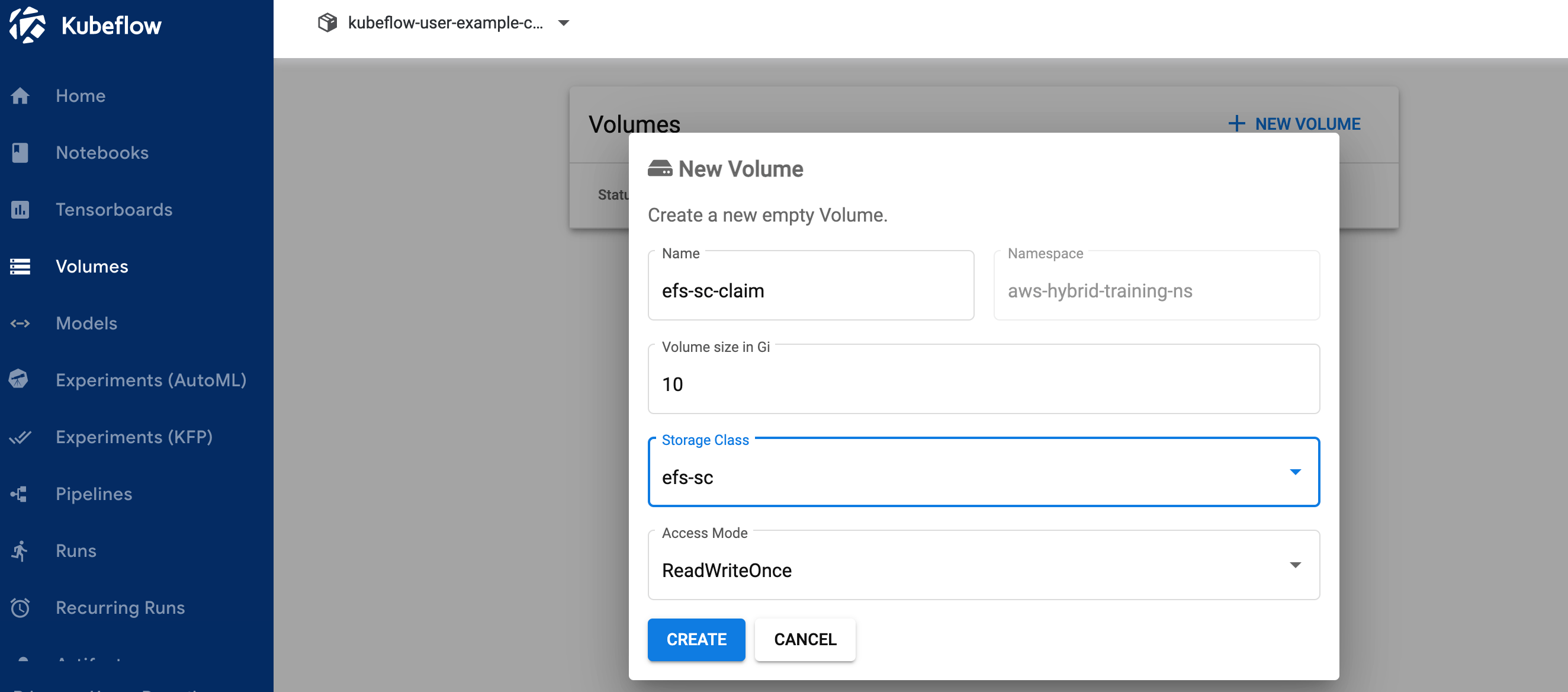
2.1 Create an EFS volume
To create an EFS volume, complete the following steps:
- On the Kubeflow dashboard, choose Volumes in the navigation pane.
- Chose New volume.
- For Name, enter
efs-sc-claim. - For Volume size, enter
10. - For Storage class, choose efs-sc.
- For Access mode, choose ReadWriteOnce.
- Choose Create.
2.2 Create a Jupyter notebook
To create a new notebook, complete the following steps:
- On the Kubeflow dashboard, choose Notebooks in the navigation pane.
- Choose New notebook.
- For Name, enter
aws-hybrid-nb. - For Jupyter Docket Image, choose the image
c9e4w0g3/notebook-servers/jupyter-pytorch:1.11.0-cpu-py38-ubuntu20.04-e3-v1.1(the latest available jupyter-pytorch DLC image). - For CPU, enter
1. - For Memory, enter
5. - For GPUs, leave as None.
- Don’t make any changes to the Workspace Volume section.
- In the Data Volumes section, choose Attach existing volume and expand Existing volume section
- For Name, choose
efs-sc-claim. - For Mount path, enter
/home/jovyan/efs-sc-claim.
This mounts the EFS volume to your Jupyter notebook pod, and you can see the folderefs-sc-claimin your Jupyter lab interface. You save the training dataset and training code to this folder so the training clusters can access it without needing to rebuild the container images for testing.
- Select Allow access to Kubeflow Pipelines in Configuration section.
- Choose Launch.
Verify that your notebook is created successfully (it may take a couple of minutes).
- On the Notebooks page, choose Connect to log in to the JupyterLab environment.
- On the Git menu, choose Clone a Repository.
- For Clone a repo, enter
https://github.com/aws-samples/aws-do-kubeflow.

3. Run distributed training
After you set up the Jupyter notebook, you can run the entire demo using the following high-level steps from the folder aws-do-kubeflow/workshop in the cloned repository:
- PyTorch Distributed Data Parallel (DDP) training Script: Refer PyTorch DDP training script cifar10-distributed-gpu-final.py, which includes a sample convolutional neural network and logic to distribute training on a multi-node CPU and GPU cluster. (Refer 3.1 for details)
-
Install libraries: Run the notebook
0_initialize_dependencies.ipynbto initialize all dependencies. (Refer 3.2 for details) -
Run distributed PyTorch job training on Kubernetes: Run the notebook
1_submit_pytorchdist_k8s.ipynbto create and submit distributed training on one primary and two worker containers using the Kubernetes custom resource PyTorchJob YAML file using Python code. (Refer 3.3 for details) -
Create a hybrid Kubeflow pipeline: Run the notebook
2_create_pipeline_k8s_sagemaker.ipynbto create the hybrid Kubeflow pipeline that runs distributed training on the either SageMaker or Amazon EKS using the runtime variabletraining_runtime. (Refer 3.4 for details)
Make sure you ran the notebook 1_submit_pytorchdist_k8s.ipynb before you start notebook 2_create_pipeline_k8s_sagemaker.ipynb.
In the subsequent sections, we discuss each of these steps in detail.
3.1 PyTorch Distributed Data Parallel(DDP) training script
As part of the distributed training, we train a classification model created by a simple convolutional neural network that operates on the CIFAR10 dataset. The training script cifar10-distributed-gpu-final.py contains only the open-source libraries and is compatible to run both on Kubernetes and SageMaker training clusters on either GPU devices or CPU instances. Let’s look at a few important aspects of the training script before we run our notebook examples.
We use the torch.distributed module, which contains PyTorch support and communication primitives for multi-process parallelism across nodes in the cluster:
We create a simple image classification model using a combination of convolutional, max pooling, and linear layers to which a relu activation function is applied in the forward pass of the model training:
We use the torch DataLoader that combines the dataset and DistributedSampler (loads a subset of data in a distributed manner using torch.nn.parallel.DistributedDataParallel) and provides a single-process or multi-process iterator over the data:
If the training cluster has GPUs, the script runs the training on CUDA devices and the device variable holds the default CUDA device:
Before you run distributed training using PyTorch DistributedDataParallel to run distributed processing on multiple nodes, you need to initialize the distributed environment by calling init_process_group. This is initialized on each machine of the training cluster.
We instantiate the classifier model and copy over the model to the target device. If distributed training is enabled to run on multiple nodes, the DistributedDataParallel class is used as a wrapper object around the model object, which allows synchronous distributed training across multiple machines. The input data is split on the batch dimension and a replica of model is placed on each machine and each device.
3.2 Install libraries
You will install all necessary libraries to run the PyTorch distributed training example. This includes Kubeflow Pipelines SDK, Training Operator Python SDK, Python client for Kubernetes and Amazon SageMaker Python SDK.
3.3 Run distributed PyTorch job training on Kubernetes
The notebook 1_submit_pytorchdist_k8s.ipynb creates the Kubernetes custom resource PyTorchJob YAML file using Kubeflow training and the Kubernetes client Python SDK. The following are a few important snippets from this notebook.
We create the PyTorchJob YAML with the primary and worker containers as shown in the following code:
This is submitted to the Kubernetes control plane using PyTorchJobClient:
View the Kubernetes training logs
You can view the training logs either from the same Jupyter notebook using Python code or from the Kubernetes client shell.
- From the notebook, run the following code with the appropriate
log_typeparameter value to view the primary, worker, or all logs: - From the Kubernetes client shell connected to the Kubernetes cluster, run the following commands using Kubectl to see the logs (substitute your namespace and pod names):

We set world size – 3 because we’re distributing the training to three processes running in one primary and two worker pods. Data is split at the batch dimension and a third of the data is processed by the model in each container.

3.4 Create a hybrid Kubeflow pipeline
The notebook 2_create_pipeline_k8s_sagemaker.ipynb creates a hybrid Kubeflow pipeline based on conditional runtime variable training_runtime, as shown in the following code. The notebook uses the Kubeflow Pipelines SDK and it’s provided a set of Python packages to specify and run the ML workflow pipelines. As part of this SDK, we use the following packages:
- The domain-specific language (DSL) package decorator
dsl.pipeline, which decorates the Python functions to return a pipeline - The
dsl.Conditionpackage, which represents a group of operations that are only run when a certain condition is met, such as checking thetraining_runtimevalue assagemakerorkubernetes
See the following code:
We configure SageMaker distributed training using two ml.p3.2xlarge instances.
After the pipeline is defined, you can compile the pipeline to an Argo YAML specification using the Kubeflow Pipelines SDK’s kfp.compiler package. You can run this pipeline using the Kubeflow Pipeline SDK client, which calls the Pipelines service endpoint and passes in appropriate authentication headers right from the notebook. See the following code:
If you get a sagemaker import error, run !pip install sagemaker and restart the kernel (on the Kernel menu, choose Restart Kernel).
Choose the Run details link under the last cell to view the Kubeflow pipeline.
Repeat the pipeline creation step with training_runtime='kubernetes' to test the pipeline run on a Kubernetes environment. The training_runtime variable can also be passed in your CI/CD pipeline in a production scenario.
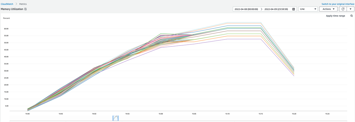
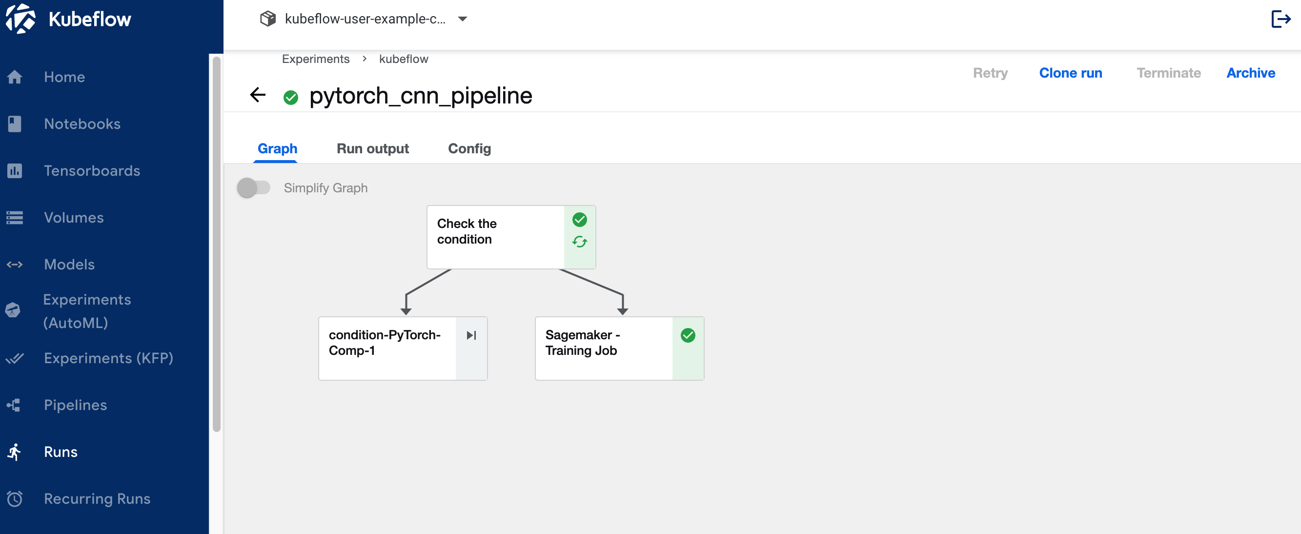
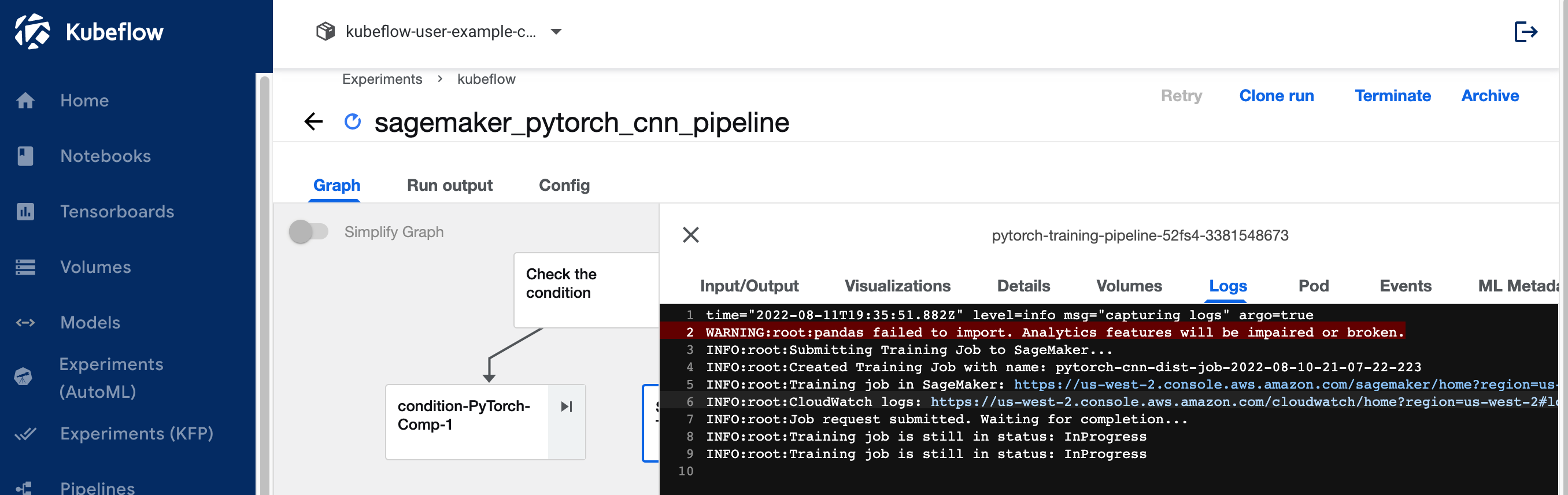
View the Kubeflow pipeline run logs for the SageMaker component
The following screenshot shows our pipeline details for the SageMaker component.
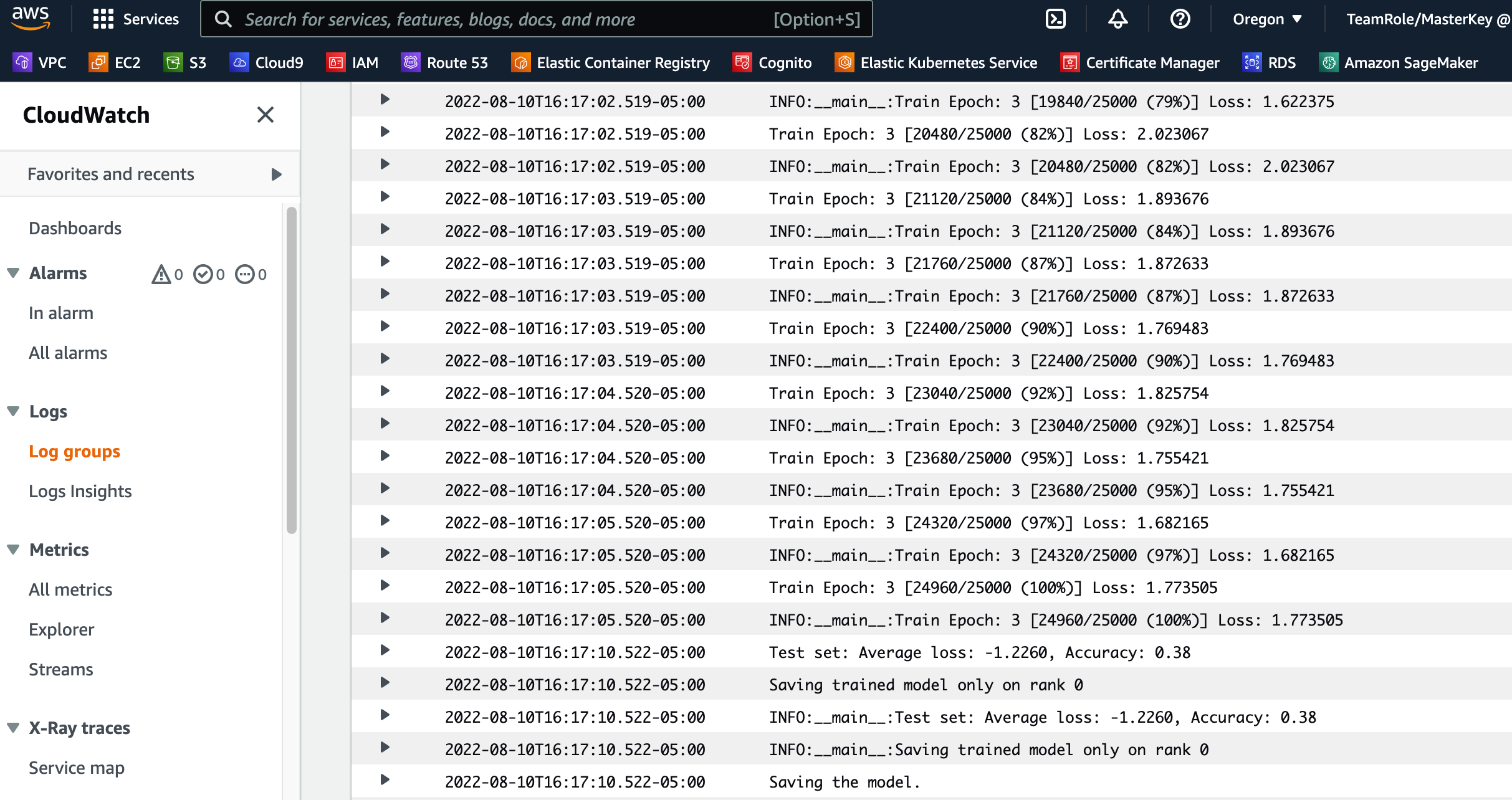
Choose the training job step and on the Logs tab, choose the CloudWatch logs link to access the SageMaker logs.
The following screenshot shows the CloudWatch logs for each of the two ml.p3.2xlarge instances.
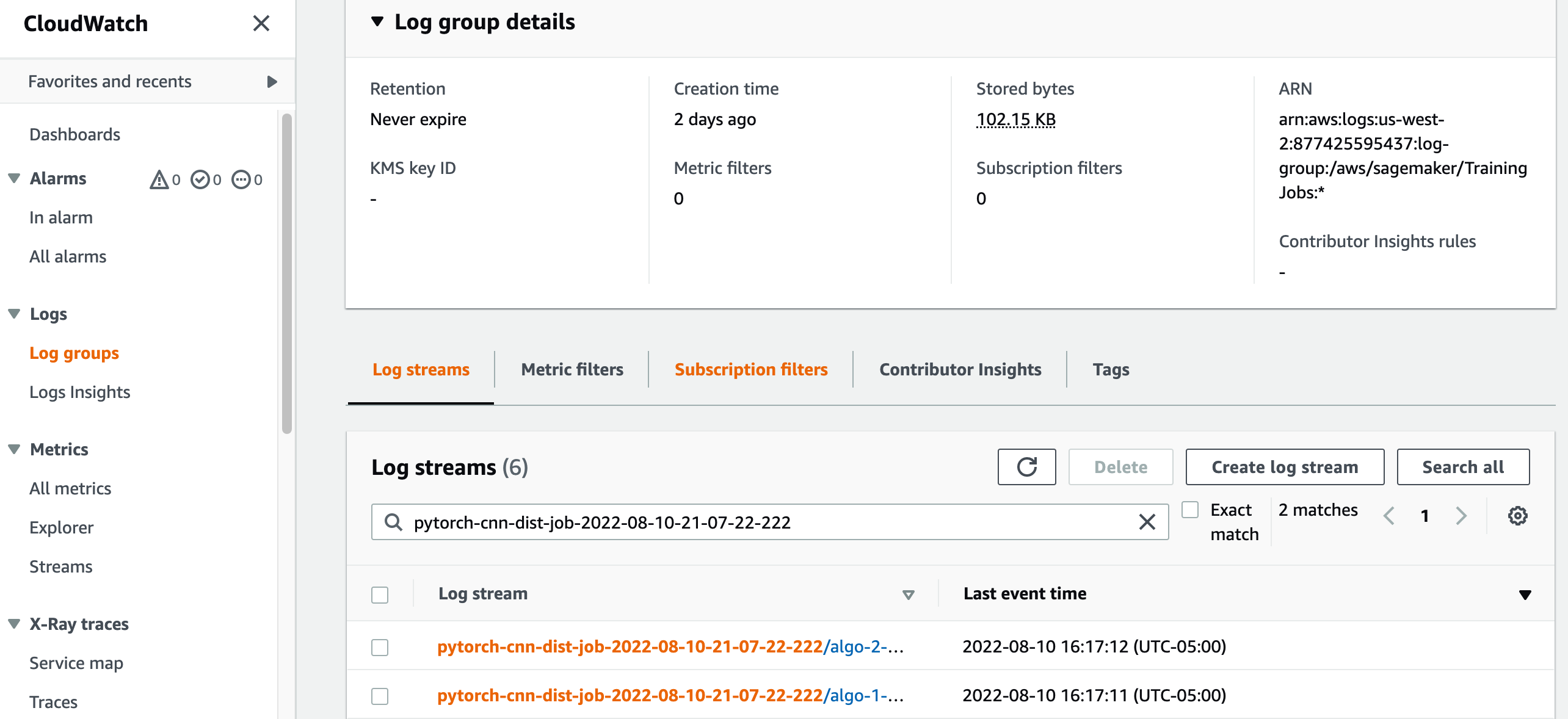
Choose any of the groups to see the logs.
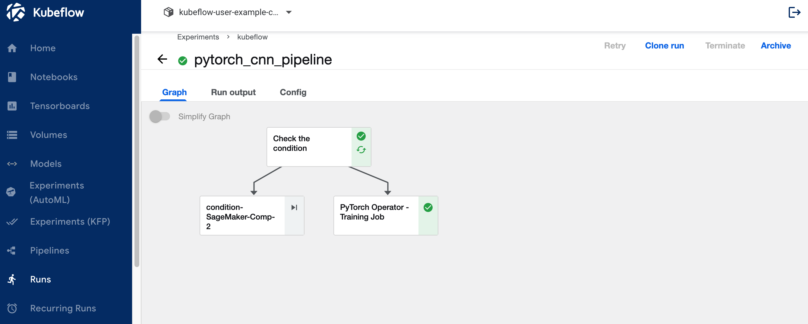
View the Kubeflow pipeline run logs for the Kubeflow PyTorchJob Launcher component
The following screenshot shows the pipeline details for our Kubeflow component.
Run the following commands using Kubectl on your Kubernetes client shell connected to the Kubernetes cluster to see the logs (substitute your namespace and pod names):
4.1 Clean up
To clean up all the resources we created in the account, we need to remove them in reverse order.
- Delete the Kubeflow installation by running
./kubeflow-remove.shin theaws-do-kubeflowcontainer. The first set of commands are optional and can be used in case you don’t already have a command shell into youraws-do-kubeflowcontainer open. - From the
aws-do-ekscontainer folder, remove the EFS volume. The first set of commands is optional and can be used in case you don’t already have a command shell into youraws-do-ekscontainer open.Deleting Amazon EFS is necessary in order to release the network interface associated with the VPC we created for our cluster. Note that deleting the EFS volume destroys any data that is stored on it.
- From the
aws-do-ekscontainer, run theeks-delete.shscript to delete the cluster and any other resources associated with it, including the VPC:
Summary
In this post, we discussed some of the typical challenges of distributed model training and ML workflows. We provided an overview of the Kubeflow on AWS distribution and shared two open-source projects (aws-do-eks and aws-do-kubeflow) that simplify provisioning the infrastructure and the deployment of Kubeflow on it. Finally, we described and demonstrated a hybrid architecture that enables workloads to transition seamlessly between running on a self-managed Kubernetes and fully managed SageMaker infrastructure. We encourage you to use this hybrid architecture for your own use cases.
You can follow the AWS Labs repository to track all AWS contributions to Kubeflow. You can also find us on the Kubeflow #AWS Slack Channel; your feedback there will help us prioritize the next features to contribute to the Kubeflow project.
Special thanks to Sree Arasanagatta (Software Development Manager AWS ML) and Suraj Kota (Software Dev Engineer) for their support to the launch of this post.
About the authors
 Kanwaljit Khurmi is an AI/ML Specialist Solutions Architect at Amazon Web Services. He works with the AWS product, engineering and customers to provide guidance and technical assistance helping them improve the value of their hybrid ML solutions when using AWS. Kanwaljit specializes in helping customers with containerized and machine learning applications.
 Gautam Kumar is a Software Engineer with AWS AI Deep Learning. He has developed AWS Deep Learning Containers and AWS Deep Learning AMI. He is passionate about building tools and systems for AI. In his spare time, he enjoy biking and reading books.
 Alex Iankoulski is a full-stack software and infrastructure architect who likes to do deep, hands-on work. He is currently a Principal Solutions Architect for Self-managed Machine Learning at AWS. In his role he focuses on helping customers with containerization and orchestration of ML and AI workloads on container-powered AWS services. He is also the author of the open source Do framework and a Docker captain who loves applying container technologies to accelerate the pace of innovation while solving the world’s biggest challenges. During the past 10 years, Alex has worked on combating climate change, democratizing AI and ML, making travel safer, healthcare better, and energy smarter.


 Geremy Cohen is a Solutions Architect with AWS where he helps customers build cutting-edge, cloud-based solutions. In his spare time, he enjoys short walks on the beach, exploring the bay area with his family, fixing things around the house, breaking things around the house, and BBQing.
 Pradeep Reddy is a Senior Product Manager in the SageMaker Low/No Code ML team, which includes SageMaker Autopilot, SageMaker Automatic Model Tuner. Outside of work, Pradeep enjoys reading, running and geeking out with palm sized computers like raspberry pi, and other home automation tech.
 Dr. John He is a senior software development engineer with Amazon AI, where he focuses on machine learning and distributed computing. He holds a PhD degree from CMU.