Posts in category: Amazon AWS

Want to accelerate machine learning (ML) innovation in your organization? Join us for 30 days of new Amazon SageMaker content designed to help you build, train, and deploy ML models faster. On April 20, we’re kicking off 30 days of hands-on workshops, Twitch sessions, Slack chats, and partner perspectives. Our goal is to connect you with AWS experts—including Greg Coquillio, the second-most influential speaker according to LinkedIn Top Voices 2020: Data Science & AI and Julien Simon, the number one AI evangelist according to AI magazine —to learn hints and tips for success with ML.

We built SageMaker from the ground up to provide every developer and data scientist with the ability to build, train, and deploy ML models quickly and at lower cost by providing the tools required for every step of the ML development lifecycle in one integrated, fully managed service. We have launched over 50 SageMaker capabilities in the past year alone, all aimed at making this process easier for our customers. The customer response to what we’re building has been incredible, making SageMaker one of the fastest growing services in AWS history.

To help you dive deep into these SageMaker innovations, we’re dedicating April 20 – May 21, 2021 to SageMaker education. Here are some must dos to add to your calendar:

• April 23 – Introduction to SageMaker workshop
• April 30 – SageMaker Fridays Twitch session with Greg Coquillio and Julien Simon on cost-optimization
• May 12 – An end-to-end tutorial on SageMaker during the workshop at the AWS Summit

Besides these virtual hands-on opportunities, we will have regular blog posts from AWS experts and our partners, including Snowflake, Tableau, Genesys, and DOMO. Bookmark the SageMaker Month webpage or sign up to our weekly newsletters so you don’t miss any of the planned activities.

But we aren’t stopping there!

To coincide with SageMaker Month, we launched new Savings Plans. The SageMaker Savings Plans offer a flexible, usage-based pricing model for SageMaker. The goal of the savings plans is to offer you the flexibility to save up to 64% on SageMaker ML instance usage in exchange for a commitment of consistent usage for a 1 or 3-year term. For more information, read the launch blog. Further, to help you save even more, we also just announced a price drop on several instance families in SageMaker.

The SageMaker Savings Plans are on top of the productivity and cost-optimizing capabilities already available in SageMaker Studio. You can improve your data science team’s productivity up to 10 times using SageMaker Studio. SageMaker Studio provides a single web-based visual interface where you can perform all your ML development steps. SageMaker Studio gives you complete access, control, and visibility into each step required to build, train, and deploy models. You can quickly upload data, create new notebooks, train and tune models, move back and forth between steps to adjust experiments, compare results, and deploy models to production all in one place, which boosts productivity.

You can also optimize costs through capabilities such as Managed Spot Training, in which you use Amazon Elastic Compute Cloud (Amazon EC2) Spot Instances for your SageMaker training jobs (see Optimizing and Scaling Machine Learning Training with Managed Spot Training for Amazon SageMaker), and Amazon Elastic Inference, which allows you to attach just the right amount of GPU-powered inference acceleration to any SageMaker instance type.

We are also excited to see continued customer momentum with SageMaker. Just in the first quarter of 2021, we launched 15 new SageMaker case studies and references, spanning a wide range industries including SNCF, Mueller, Bundesliga, University of Oxford, and Latent Space. Some highlights include:

• The data science team at SNFC reduced model training time from 3 days to 10 hours.
• Mueller Water Products automated the daily collection of more than 5 GB of data and used ML to improve leak-detection performance.
• Latent Space scaled model training beyond 1 billion parameters.

We would love for you to join the thousands of customers who are seeing success with Amazon SageMaker. We want to add you to our customer reference list, and we can’t wait to work with you this month!

About the Author

Kimberly Madia is a Principal Product Marketing Manager with AWS Machine Learning. Her goal is to make it easy for customers to build, train, and deploy machine learning models using Amazon SageMaker. For fun outside work, Kimberly likes to cook, read, and run on the San Francisco Bay Trail.

Read More

You can now control the Amazon Virtual Private Cloud (Amazon VPC) and encryption settings for your Amazon Comprehend APIs using AWS Identity and Access Management (IAM) condition keys, and encrypt your Amazon Comprehend custom models using customer managed keys (CMK) via AWS Key Management Service (AWS KMS). IAM condition keys enable you to further refine the conditions under which an IAM policy statement applies. You can use the new condition keys in IAM policies when granting permissions to create asynchronous jobs and creating custom classification or custom entity training jobs.

Amazon Comprehend now supports five new condition keys:

• comprehend:VolumeKmsKey
• comprehend:OutputKmsKey
• comprehend:ModelKmsKey
• comprehend:VpcSecurityGroupIds
• comprehend:VpcSubnets

The keys allow you to ensure that users can only create jobs that meet your organization’s security posture, such as jobs that are connected to the allowed VPC subnets and security groups. You can also use these keys to enforce encryption settings for the storage volumes where the data is pulled down for computation and on the Amazon Simple Storage Service (Amazon S3) bucket where the output of the operation is stored. If users try to use an API with VPC settings or encryption parameters that aren’t allowed, Amazon Comprehend rejects the operation synchronously with a 403 Access Denied exception.

Solution overview

The following diagram illustrates the architecture of our solution.

We want to enforce a policy to do the following:

• Make sure that all custom classification training jobs are specified with VPC settings
• Have encryption enabled for the classifier training job, the classifier output, and the Amazon Comprehend model

This way, when someone starts a custom classification training job, the training data that is pulled in from Amazon S3 is copied to the storage volumes in your specified VPC subnets and is encrypted with the specified VolumeKmsKey. The solution also makes sure that the results of the model training are encrypted with the specified OutputKmsKey. Finally, the Amazon Comprehend model itself is encrypted with the AWS KMS key specified by the user when it’s stored within the VPC. The solution uses three different keys for the data, output, and the model, respectively, but you can choose to use the same key for all three tasks.

Additionally, this new functionality enables you to audit model usage in AWS CloudTrail by tracking the model encryption key usage.

Encryption with IAM policies

The following policy makes sure that users must specify VPC subnets and security groups for VPC settings and AWS KMS keys for both the classifier and output:

{
   "Version": "2012-10-17",
   "Statement": [{
    "Action": ["comprehend:CreateDocumentClassifier"],
    "Effect": "Allow",
    "Resource": "*",
    "Condition": {
      "Null": {
        "comprehend:VolumeKmsKey": "false",
        "comprehend:OutputKmsKey": "false",
        "comprehend:ModelKmsKey": "false",
        "comprehend:VpcSecurityGroupIds": "false",
        "comprehend:VpcSubnets": "false"
      }
    }
  }]
}

For example, in the following code, User 1 provides both the VPC settings and the encryption keys, and can successfully complete the operation:

aws comprehend create-document-classifier 
--region region 
--document-classifier-name testModel 
--language-code en 
--input-data-config S3Uri=s3://S3Bucket/docclass/filename 
--data-access-role-arn arn:aws:iam::[your account number]:role/testDataAccessRole
--volume-kms-key-id arn:aws:kms:region:[your account number]:alias/ExampleAlias
--output-data-config S3Uri=s3://S3Bucket/output/file name,KmsKeyId=arn:aws:kms:region:[your account number]:alias/ExampleAlias
--vpc-config SecurityGroupIds=sg-11a111111a1exmaple,Subnets=subnet-11aaa111111example

User 2, on the other hand, doesn’t provide any of these required settings and isn’t allowed to complete the operation:

aws comprehend create-document-classifier 
--region region 
--document-classifier-name testModel 
--language-code en 
--input-data-config S3Uri=s3://S3Bucket/docclass/filename 
--data-access-role-arn arn:aws:iam::[your account number]:role/testDataAccessRole
--output-data-config S3Uri=s3://S3Bucket/output/file name

In the preceding code examples, as long as the VPC settings and the encryption keys are set, you can run the custom classifier training job. Leaving the VPC and encryption settings in their default state results in a 403 Access Denied exception.

In the next example, we enforce an even stricter policy, in which we have to set the VPC and encryption settings to also include specific subnets, security groups, and KMS keys. This policy applies these rules for all Amazon Comprehend APIs that start new asynchronous jobs, create custom classifiers, and create custom entity recognizers. See the following code:

{
   "Version": "2012-10-17",
   "Statement": [{
    "Action":
     [
    "comprehend:CreateDocumentClassifier",
    "comprehend:CreateEntityRecognizer",
    "comprehend:Start*Job"
    ],
    "Effect": "Allow",
    "Resource": "*",
    "Condition": {
      "ArnEquals": {
        "comprehend:VolumeKmsKey": "arn:aws:kms:region:[your account number]:key/key_id",
        "comprehend:ModelKmsKey": "arn:aws:kms:region:[your account number]:key/key_id1",
        "comprehend:OutputKmsKey": "arn:aws:kms:region:[your account number]:key/key_id2"
      },
      "ForAllValues:StringLike": {
        "comprehend:VpcSecurityGroupIds": [
          "sg-11a111111a1exmaple"
        ],
        "comprehend:VpcSubnets": [
          "subnet-11aaa111111example"
        ]
      }
    }
  }]
}

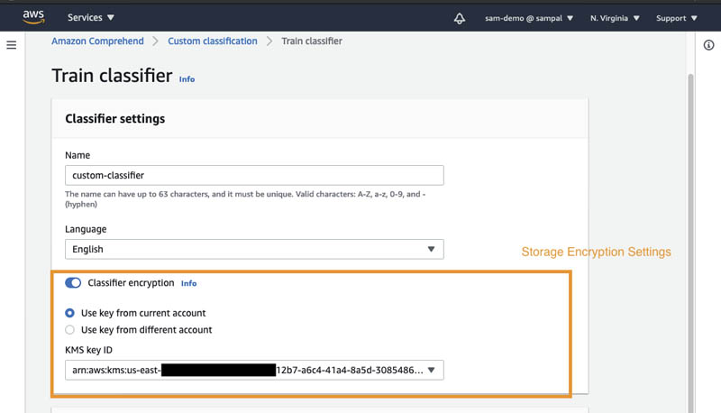
In the next example, we first create a custom classifier on the Amazon Comprehend console without specifying the encryption option. Because we have the IAM conditions specified in the policy, the operation is denied.

When you enable classifier encryption, Amazon Comprehend encrypts the data in the storage volume while your job is being processed. You can either use an AWS KMS customer managed key from your account or a different account. You can specify the encryption settings for the custom classifier job as in the following screenshot.

Output encryption enables Amazon Comprehend to encrypt the output results from your analysis. Similar to Amazon Comprehend job encryption, you can either use an AWS KMS customer managed key from your account or another account.

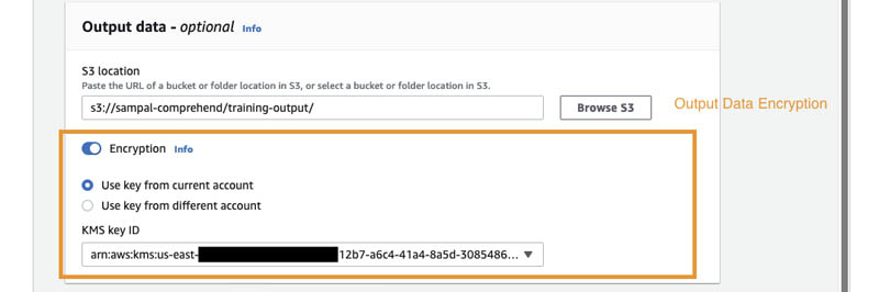
Because our policy also enforces the jobs to be launched with VPC and security group access enabled, you can specify these settings in the VPC settings section.

Amazon Comprehend API operations and IAM condition keys

The following table lists the Amazon Comprehend API operations and the IAM condition keys that are supported as of this writing. For more information, see Actions, resources, and condition keys for Amazon Comprehend.

Model encryption with a CMK

Along with encrypting your training data, you can now encrypt your custom models in Amazon Comprehend using a CMK. In this section, we go into more detail about this feature.

Prerequisites

You need to add an IAM policy to allow a principal to use or manage CMKs. CMKs are specified in the Resource element of the policy statement. When writing your policy statements, it’s a best practice to limit CMKs to those that the principals need to use, rather than give the principals access to all CMKs.

In the following example, we use an AWS KMS key (1234abcd-12ab-34cd-56ef-1234567890ab) to encrypt an Amazon Comprehend custom model.

When you use AWS KMS encryption, kms:CreateGrant and kms:RetireGrant permissions are required for model encryption.

For example, the following IAM policy statement in your dataAccessRole provided to Amazon Comprehend allows the principal to call the create operations only on the CMKs listed in the Resource element of the policy statement:

{"Version": "2012-10-17",
  "Statement": {"Effect": "Allow",
    "Action": [
      "kms:CreateGrant",
      "kms:RetireGrant",
      "kms:GenerateDataKey",
      "kms:Decrypt"
    ],
    "Resource": [
      "arn:aws:kms:us-west-2:[your account number]:key/1234abcd-12ab-34cd-56ef-1234567890ab"
    ]
  }
}

Specifying CMKs by key ARN, which is a best practice, makes sure that the permissions are limited only to the specified CMKs.

Enable model encryption

As of this writing, custom model encryption is available only via the AWS Command Line Interface (AWS CLI). The following example creates a custom classifier with model encryption:

 aws comprehend create-document-classifier 
--document-classifier-name my-document-classifier  
--data-access-role-arn arn:aws:iam::[your account number]:role/mydataaccessrole 
--language-code en  --region us-west-2 
--model-kms-key-id arn:aws:kms:us-west-2:[your account number]:key/[your key Id] 
--input-data-config S3Uri=s3://path-to-data/multiclass_train.csv

The next example trains a custom entity recognizer with model encryption:

aws comprehend create-entity-recognizer 
--recognizer-name my-entity-recognizer 
--data-access-role-arn arn:aws:iam::[your account number]:role/mydataaccessrole  
--language-code "en" --region us-west-2 
--input-data-config '{
      "EntityTypes": [{"Type": "PERSON"}, {"Type": "LOCATION"}],
      "Documents": {
            "S3Uri": "s3://path-to-data/documents"
      },
      "Annotations": {
          "S3Uri": "s3://path-to-data/annotations"
      }
}'

Finally, you can also create an endpoint for your custom model with encryption enabled:

aws comprehend create-endpoint 
 --endpoint-name myendpoint 
 --model-arn arn:aws:comprehend:us-west-2:[your account number]:document-classifier/my-document-classifier 
 --data-access-role-arn arn:aws:iam::[your account number]:role/mydataaccessrole 
 --desired-inference-units 1 --region us-west-2

Conclusion

You can now enforce security settings like enabling encryption and VPC settings for your Amazon Comprehend jobs using IAM condition keys. The IAM condition keys are available in all AWS Regions where Amazon Comprehend is available. You can also encrypt the Amazon Comprehend custom models using customer managed keys.

To learn more about the new condition keys and view policy examples, see Using IAM condition keys for VPC settings and Resource and Conditions for Amazon Comprehend APIs. To learn more about using IAM condition keys, see IAM JSON policy elements: Condition.

About the Authors

Sam Palani is an AI/ML Specialist Solutions Architect at AWS. He enjoys working with customers to help them architect machine learning solutions at scale. When not helping customers, he enjoys reading and exploring the outdoors.

Shanthan Kesharaju is a Senior Architect in the AWS ProServe team. He helps our customers with AI/ML strategy, architecture, and developing products with a purpose. Shanthan has an MBA in Marketing from Duke University and an MS in Management Information Systems from Oklahoma State University.

Read More

In preparation for the upcoming Olympic Games, Intel®, an American multinational corporation and one of the world’s largest technology companies, developed a concept around 3D Athlete Tracking (3DAT). 3DAT is a machine learning (ML) solution to create real-time digital models of athletes in competition in order to increase fan engagement during broadcasts. Intel was looking to leverage this technology for the purpose of coaching and training elite athletes.

Classical computer vision methods for 3D pose reconstruction have proven to be cumbersome for most scientists, given that these models mostly rely on embedding additional sensors on an athlete and the lack of 3D labels and models. Although we can put seamless data collection mechanisms in place using regular mobile phones, developing 3D models using 2D video data is a challenge, given the lack of depth of information in 2D videos. Intel’s 3DAT team partnered with the Amazon ML Solutions Lab (MLSL) to develop 3D human pose estimation techniques on 2D videos in order to create a lightweight solution for coaches to extract biomechanics and other metrics of their athletes’ performance.

This unique collaboration brought together Intel’s rich history in innovation and Amazon ML Solution Lab’s computer vision expertise to develop a 3D multi-person pose estimation pipeline using 2D videos from standard mobile phones as inputs, with Amazon SageMaker Studio notebooks (SM Studio) as the development environment.

Jonathan Lee, Director of Intel Sports Performance, Olympic Technology Group, says, “The MLSL team did an amazing job listening to our requirements and proposing a solution that would meet our customers’ needs. The team surpassed our expectations, developing a 3D pose estimation pipeline using 2D videos captured with mobile phones in just two weeks. By standardizing our ML workload on Amazon SageMaker, we achieved a remarkable 97% average accuracy on our models.”

This post discusses how we employed 3D pose estimation models and generated 3D outputs on 2D video data collected from Ashton Eaton, a decathlete and two-time Olympic gold medalist from the United States, using different angles. It also presents two computer vision techniques to align the videos captured from different angles, thereby allowing coaches to use a unique set of 3D coordinates across the run.

Challenges

Human pose estimation techniques use computer vision aim to provide a graphical skeleton of a person detected in a scene. They include coordinates of predefined key points corresponding to human joints, such as the arms, neck, and hips. These coordinates are used to capture the body’s orientation for further analysis, such as pose tracking, posture analysis, and subsequent evaluation. Recent advances in computer vision and deep learning have enabled scientists to explore pose estimation in a 3D space, where the Z-axis provides additional insights compared to 2D pose estimation. These additional insights could be used for more comprehensive visualization and analysis. However, building a 3D pose estimation model from scratch is challenging because it requires imaging data along with 3D labels. Therefore, many researchers employ pretrained 3D pose estimation models.

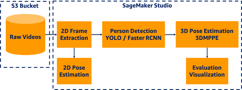
Data processing pipeline

We designed an end-to-end 3D pose estimation pipeline illustrated in the following diagram using SM Studio, which encompassed several components:

• Amazon Simple Storage Service (Amazon S3) bucket to host video data
• Frame extraction module to convert video data to static images
• Object detection modules to detect bounding boxes of persons in each frame
• 2D pose estimation for future evaluation purposes
• 3D pose estimation module to generate 3D coordinates for each person in each frame
• Evaluation and visualization modules

SM Studio offers a broad range of features facilitating the development process, including easy access to data in Amazon S3, availability of compute capability, software and library availability, and an integrated development experience (IDE) for ML applications.

First, we read the video data from the S3 bucket and extracted the 2D frames in a portable network graphics (PNG) format for frame-level development. We used YOLOv3 object detection to generate a bounding box of each person detected in a frame. For more information, see Benchmarking Training Time for CNN-based Detectors with Apache MXNet.

Next, we passed the frames and corresponding bounding box information to the 3D pose estimation model to generate the key points for evaluation and visualization. We applied a 2D pose estimation technique to the frames, and we generated the key points per frame for development and evaluation. The following sections discuss the details of each module in the 3D pipeline.

Data preprocessing

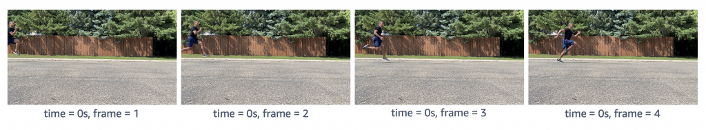
The first step was to extract frames from a given video utilizing OpenCV as shown in the following figure. We used two counters to keep track of time and frame count respectively, because videos were captured at different frames per second (FPS) rates. We then stored the sequence of images asvideo_name + second_count + frame_countin PNG format.

Object (person) detection

We employed YOLOv3 pretrained models based on the Pascal VOC dataset to detect persons in frames. For more information, see Deploying custom models built with Gluon and Apache MXNet on Amazon SageMaker. The YOLOv3 algorithm produced the bounding boxes shown in the following animations (the original images are resized to 910×512 pixels).

We stored the bounding box coordinates in a CSV file, in which the rows indicated the frame index, bounding box information as a list, and their confidence scores.

2D pose estimation

We selected ResNet-18 V1b as the pretrained pose estimation model, which considers a top-down strategy to estimate human poses within bounding boxes output by the object detection model. We further reset the detector classes to include humans so that the non-maximum suppression (NMS) process could be performed faster. The Simple Pose network was applied to predict heatmaps for key points (as in the following animation), and the highest values in the heatmaps were mapped to the coordinates on the original images.

3D pose estimation

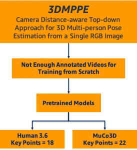
We employed a state-of-the-art 3D pose estimation algorithm encompassing a camera distance-aware top-down method for multi-person per RGB frame referred to as 3DMPPE (Moon et al.). This algorithm consisted of two major phases:

• RootNet – Estimates the camera-centered coordinates of a person’s root in a cropped frame
• PoseNet – Uses a top-down approach to predict the relative 3D pose coordinates in the cropped image

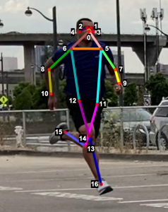
Next, we used the bounding box information to project the 3D coordinates back to the original space. 3DMPPE offered two pretrained models trained using Human36 and MuCo3D datasets (for more information, see the GitHub repo), which included 17 and 21 key points, respectively, as illustrated in the following animations. We used the 3D pose coordinates predicted by the two pretrained models for visualization and evaluation purposes.

Evaluation

To evaluate the 2D and 3D pose estimation models’ performance, we used the 2D pose (x,y) and 3D pose (x,y,z) coordinates for each joint generated for every frame in a given video. The number of key points varied based on the datasets; for instance, the Leeds Sports Pose Dataset (LSP) includes 14, whereas the MPII Human Pose dataset, a state-of-the-art benchmark for evaluating articulated human pose estimation referring to Human3.6M, includes 16 key points. We used two metrics commonly used for both 2D and 3D pose estimation, as described in the next section on evaluation. In our implementation, our default key points dictionary followed the COCO detection dataset, which has 17 key points (see the following image), and the order is defined as follows:

KEY POINTS = {
    0: "nose",
    1: "left_eye",
    2: "right_eye",
    3: "left_ear",
    4: "right_ear",
    5: "left_shoulder",
    6: "right_shoulder",
    7: "left_elbow",
    8: "right_elbow",
    9: "left_wrist",
    10: "right_wrist",
    11: "left_hip",
    12: "right_hip",
    13: "left_knee",
    14: "right_knee",
    15: "left_ankle",
    16: "right_ankle"
}

Mean per joint position error

Mean per joint position error (MPJPE) is the Euclidean distance between ground truth and a joint prediction. As MPJPE measures the error or loss distance, and lower values indicate greater precision.

We use the following pseudo code:

• Let G denote ground_truth_joint and preprocess G by:
  • Replacing the null entries in G with [0,0] (2D) or [0,0,0] (3D)
  • Using a Boolean matrix B to store the location of null entries
• Let P denote predicted_joint matrix, and align G and P by frame index by inserting a zero vector if any frame doesn’t have results or is unlabeled
• Compute element-wise Euclidean distance between G and P, and let D denote distance matrix
• Replace D_i,j with 0 if B_i,j
• Mean per joint position is the mean value of each column of D_s,tD_i,j ≠ 0

The following figure visualizes an example of video’s per joint error, a matrix with dimension m*n, where m denotes the number of frames in a video and n denotes the number of joints (key points). The matrix shows an example of a heatmap of per joint position error on the left and the mean per joint position error on the right.

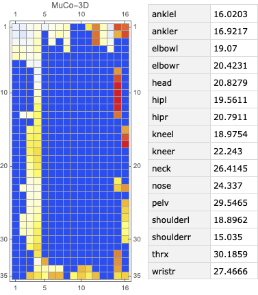
The following figure visualizes an example of video’s per joint error, a matrix with dimension m*n , where m denotes the number of frames in a video and n denotes the number of joints (key points). The matrix shows an example of a heatmap of per joint position error on the left and the mean per joint position error on the right.

Percentage of correct key points

The percentage of correct key points (PCK) represents a pose evaluation metric where a detected joint is considered correct if the distance between the predicted and actual joint is within a certain threshold; this threshold may vary, which leads to a few different variations of metrics. Three variations are commonly used:

• PCKh@0.5, which is when the threshold is defined as 0.5 * head bone link
• PCK@0.2, which is when the distance between the predicted and actual joint is < 0.2 * torso diameter
• 150mm as a hard threshold

In our solution, we used the PCKh@0.5 as our ground truth XML data containing the head bounding box, which we can use to compute the head-bone link. To the best of our knowledge, no existing package contains an easy-to-use implementation for this metric; therefore, we implemented the metric in-house.

Pseudo code

We used the following pseudo code:

• Let G denote ground-truth joint and preprocess G by:
  • Replacing the null entries in G with [0,0] (2D) or [0,0,0] (3D)
  • Using a Boolean matrix B to store the location of null entries
• For each frame F_i, use its bbox B_i=(x_min,y_min,x_max,y_max) to compute each frame’s corresponding head-bone link H_i , where H_i=((x_max-x_min)²+(y_max-y_min)²)^½
• Let P denote predicted joint matrix and align G and P by frame index; insert a zero tensor if any frame is missing
• Compute the element-wise 2-norm error between G and P; let E denote error matrix, where E_i,j=||G_i,j-P_i,j||
• Compute a scaled matrix S=H*I, where I represents an identity matrix with the same dimension as E
• To avoid division by 0, replace S_i,j with 0.000001 if B_i,j=1
• Compute scaled error matrix S_i,j=E_i,j/S_i,j
• Filter out SE with threshold = 0.5, and let C denote the counter matrix, where C_i,j=1 if SE_i,j<0.5 and C_i,j=0 elsewise
• Count how many 1’s in C_*,j as c⃗ and count how many 0’s in B_*,j as b⃗
• PCKh@0.5=mean(c⃗/b⃗)

In the sixth step (replace S_i,jwith 0.000001 if B_i,j=1), we set up a trap for the scaled error matrix by replacing 0 entries with 0.00001. Dividing any number by a tiny number generates an amplified number. Because we later used > 0.5 as a threshold to filter out incorrect predictions, the null entries were excluded from the correct prediction because it was way too large. We subsequently counted only the not null entries in the Boolean matrix. In this way, we also excluded the null entries from the whole dataset. We proposed an engineering trick in this implementation to filter out null entries from either unlabeled key points in the ground truth or the frames with no person detected.

Video alignment

We considered two different camera configurations to capture video data from athletes, namely the line and box setups. The line setup consists of four cameras placed along a line while the box setup consists of four cameras placed in each corner of a rectangle. The cameras were synchronized in the line configuration and then lined up at a predefined distance from each other, utilizing slightly overlapping camera angles. The objective of the video alignment in the line configuration was to identify the timestamps connecting consecutive cameras to remove repeated and empty frames. We implemented two approaches based on object detection and cross-correlation of optical flows.

Object detection algorithm

We used the object detection results in this approach, including persons’ bounding boxes from the previous steps. The object detection techniques produced a probability (score) per person in each frame. Therefore, plotting the scores in a video enabled us to find the frame where the first person appeared or disappeared. The reference frame from the box configuration was extracted from each video, and all cameras were then synchronized based on the first frame’s references. In the line configuration, both the start and end timestamps were extracted, and a rule-based algorithm was implemented to connect and align consecutive videos, as illustrated in the following images.

The top videos in the following figure show the original videos in the line configuration. Underneath that are person detection scores. The next rows show a threshold of 0.75 applied to the scores, and appropriate start and end timestamps are extracted. The bottom row shows aligned videos for further analysis.

Moment of snap

We introduced the moment of snap (MOS) – a well-known alignment approach – which indicates when an event or play begins. We wanted to determine the frame number when an athlete enters or leaves the scene. Typically, relatively little movement occurs on the running field before the start and after the end of the snap, whereas relatively substantial movement occurs when the athlete is running. Therefore, intuitively, we could find the MOS frame by finding the video frames with relatively large differences in the video’s movement before and after the frame. To this end, we utilized density optical flow, a standard measure of movement in the video, to estimate the MOS. First, given a video, we computed optical flow for every two consecutive frames. The following videos present a visualization of dense optical flow on the horizontal axis.

We then measured cross-correlation between two consecutive frames’ optical flows, because cross-correlation measures the difference between them. For each angle’s camera-captured video, we repeated the algorithm to find its MOS. Finally, we used the MOS frame as the key frame for aligning videos from different angles. The following video details these steps.

Conclusion

The technical objective of the work demonstrated in this post was to develop a deep-learning based solution producing 3D pose estimation coordinates using 2D videos. We employed a camera distance-aware technique with a top-down approach to achieve 3D multi-person pose estimation. Further, using object detection, cross-correlation, and optical flow algorithms, we aligned the videos captured from different angles.

This work has enabled coaches to analyze 3D pose estimation of athletes over time to measure biomechanics metrics, such as velocity, and monitor the athletes’ performance using quantitative and qualitative methods.

This post demonstrated a simplified process for extracting 3D poses in real-world scenarios, which can be scaled to coaching in other sports such as swimming or team sports.

If you would like help with accelerating the use of ML in your products and services, please contact the Amazon ML Solutions Lab program.

References

Moon, Gyeongsik, Ju Yong Chang, and Kyoung Mu Lee. “Camera distance-aware top-down approach for 3d multi-person pose estimation from a single RGB image.” In Proceedings of the IEEE International Conference on Computer Vision, pp. 10133-10142. 2019.

About the Author

Saman Sarraf is a Data Scientist at the Amazon ML Solutions Lab. His background is in applied machine learning including deep learning, computer vision, and time series data prediction.

Amery Cong is an Algorithms Engineer at Intel, where he develops machine learning and computer vision technologies to drive biomechanical analyses at the Olympic Games. He is interested in quantifying human physiology with AI, especially in a sports performance context.

Ashton Eaton is a Product Development Engineer at Intel, where he helps design and test technologies aimed at advancing sport performance. He works with customers and the engineering team to identify and develop products that serve customer needs. He is interested in applying science and technology to human performance.

Jonathan Lee is the Director of Sports Performance Technology, Olympic Technology Group at Intel. He studied the application of machine learning to health as an undergrad at UCLA and during his graduate work at University of Oxford. His career has focused on algorithm and sensor development for health and human performance. He now leads the 3D Athlete Tracking project at Intel.

Nelson Leung is the Platform Architect in the Sports Performance CoE at Intel, where he defines end-to-end architecture for cutting-edge products that enhance athlete performance. He also leads the implementation, deployment and productization of these machine learning solutions at scale to different Intel partners.

Suchitra Sathyanarayana is a manager at the Amazon ML Solutions Lab, where she helps AWS customers across different industry verticals accelerate their AI and cloud adoption. She holds a PhD in Computer Vision from Nanyang Technological University, Singapore.

Wenzhen Zhu is a data scientist with the Amazon ML Solution Lab team at Amazon Web Services. She leverages Machine Learning and Deep Learning to solve diverse problems across industries for AWS customers.

Read More

Customers often ask us how can they lower their costs when conducting deep learning training on AWS. Training deep learning models with libraries such as TensorFlow, PyTorch, and Apache MXNet usually requires access to GPU instances, which are AWS instances types that provide access to NVIDIA GPUs with thousands of compute cores. GPU instance types can be more expensive than other Amazon Elastic Compute Cloud (Amazon EC2) instance types, so optimizing usage of these types of instances is a priority for customers as well as an overall best practice for well-architected workloads.

Amazon SageMaker is a fully managed service that provides every developer and data scientist with the ability to prepare, build, train, and deploy machine learning (ML) models quickly. SageMaker removes the heavy lifting from each step of the ML process to make it easier to develop high-quality models. SageMaker provides all the components used for ML in a single toolset so models get to production faster with less effort and at lower cost.

Amazon EC2 Spot Instances offer spare compute capacity available in the AWS Cloud at steep discounts compared to On-Demand prices. Amazon EC2 can interrupt Spot Instances with 2 minutes of notification when the service needs the capacity back. You can use Spot Instances for various fault-tolerant and flexible applications. Some examples are analytics, containerized workloads, stateless web servers, CI/CD, training and inference of ML models, and other test and development workloads. Spot Instance pricing makes high-performance GPUs much more affordable for deep learning researchers and developers who run training jobs.

One of the key benefits of SageMaker is that it frees you of any infrastructure management, no matter the scale you’re working at. For example, instead of having to set up and manage complex training clusters, you simply tell SageMaker which EC2 instance type to use and how many you need. The appropriate instances are then created on-demand, configured, and stopped automatically when the training job is complete. As SageMaker customers have quickly understood, this means that they pay only for what they use. Building, training, and deploying ML models are billed by the second, with no minimum fees, and no upfront commitments. SageMaker can also use EC2 Spot Instances for training jobs, which optimize the cost of the compute used for training deep-learning models.

In this post, we walk through the process of training a TensorFlow model with Managed Spot Training in SageMaker. We walk through the steps required to set up and run a training job that saves training progress in Amazon Simple Storage Service (Amazon S3) and restarts the training job from the last checkpoint if an EC2 instance is interrupted. This allows our training jobs to continue from the same point before the interruption occurred. Finally, we see the savings that we achieved by running our training job on Spot Instances using Managed Spot Training in SageMaker.

Managed Spot Training in SageMaker

SageMaker makes it easy to train ML models using managed EC2 Spot Instances. Managed Spot Training can optimize the cost of training models up to 90% over On-Demand Instances. With only a few lines of code, SageMaker can manage Spot interruptions on your behalf.

Managed Spot Training uses EC2 Spot Instances to run training jobs instead of On-Demand Instances. You can specify which training jobs use Spot Instances and a stopping condition that specifies how long SageMaker waits for a training job to complete using EC2 Spot Instances. Metrics and logs generated during training runs are available in Amazon CloudWatch.

Managed Spot Training is available in all training configurations:

• All instance types supported by SageMaker
• All models: built-in algorithms, built-in frameworks, and custom models
• All configurations: single instance training and distributed training

Interruptions and checkpointing

There’s an important difference when working with Managed Spot Training. Unlike On-Demand Instances that are expected to be available until a training job is complete, Spot Instances may be reclaimed any time Amazon EC2 needs the capacity back.

SageMaker, as a fully managed service, handles the lifecycle of Spot Instances automatically. It interrupts the training job, attempts to obtain Spot Instances again, and either restarts or resumes the training job.

To avoid restarting a training job from scratch if it’s interrupted, we strongly recommend that you implement checkpointing, a technique that saves the model in training at periodic intervals. When you use checkpointing, you can resume a training job from a well-defined point in time, continuing from the most recent partially trained model, and avoiding starting from the beginning and wasting compute time and money.

To implement checkpointing, we have to make a distinction on the type of algorithm you use:

• Built-in frameworks and custom models – You have full control over the training code. Just make sure that you use the appropriate APIs to save model checkpoints to Amazon S3 regularly, using the location you defined in the CheckpointConfig parameter and passed to the SageMaker Estimator. TensorFlow uses checkpoints by default. For other frameworks, see our sample notebooks and Use Machine Learning Frameworks, Python, and R with Amazon SageMaker.
• Built-in algorithms – Computer vision algorithms support checkpointing (object detection, semantic segmentation, and image classification). Because they tend to train on large datasets and run for longer than other algorithms, they have a higher likelihood of being interrupted. The XGBoost built-in algorithm also supports checkpointing.

TensorFlow image classification model with Managed Spot Training

To demonstrate Managed Spot Training and checkpointing, I guide you through the steps needed to train a TensorFlow image classification model. To make sure that your training scripts can take advantage of SageMaker Managed Spot Training, we need to implement the following:

• Frequent saving of checkpoints, thereby saving checkpoints each epoch
• The ability to resume training from checkpoints if checkpoints exist

Save checkpoints

SageMaker automatically backs up and syncs checkpoint files generated by your training script to Amazon S3. Therefore, you need to make sure that your training script saves checkpoints to a local checkpoint directory on the Docker container that’s running the training. The default location to save the checkpoint files is /opt/ml/checkpoints, and SageMaker syncs these files to the specific S3 bucket. Both local and S3 checkpoint locations are customizable.

Saving checkpoints using Keras is very easy. You need to create an instance of the ModelCheckpoint callback class and register it with the model by passing it to the fit() function.

You can find the full implementation code on the GitHub repo.

The following is the relevant code:

callbacks = []
callbacks.append(ModelCheckpoint(args.checkpoint_path + '/checkpoint-{epoch}.h5'))

logging.info("Starting training from epoch: {}".format(initial_epoch_number+1))
    
model.fit(x=train_dataset[0],
          y=train_dataset[1],
          steps_per_epoch=(num_examples_per_epoch('train') 
          epochs=args.epochs,
          initial_epoch=initial_epoch_number,
          validation_data=validation_dataset,
          validation_steps=(num_examples_per_epoch('validation') 
          callbacks=callbacks) 

The names of the checkpoint files saved are as follows: checkpoint-1.h5, checkpoint-2.h5, checkpoint-3.h5, and so on.

For this post, I’m passing initial_epoch, which you normally don’t set. This lets us resume training from a certain epoch number and comes in handy when you already have checkpoint files.

The checkpoint path is configurable because we get it from args.checkpoint_path in the main function:

if __name__ == '__main__':
    parser = argparse.ArgumentParser()
    
    ...
    parser.add_argument("--checkpoint-path",type=str,default="/opt/ml/checkpoints",help="Path where checkpoints will be saved.")
    ...
    
    args = parser.parse_args()

Resume training from checkpoint files

When Spot capacity becomes available again after Spot interruption, SageMaker launches a new Spot Instance, instantiates a Docker container with your training script, copies your dataset and checkpoint files from Amazon S3 to the container, and runs your training scripts.

Your script needs to implement resuming training from checkpoint files, otherwise your training script restarts training from scratch. You can implement a load_model_from_checkpoints function as shown in the following code. It takes in the local checkpoint files path (/opt/ml/checkpoints being the default) and returns a model loaded from the latest checkpoint and the associated epoch number.

You can find the full implementation code on the GitHub repo.

The following is the relevant code:

def load_model_from_checkpoints(checkpoint_path):
    checkpoint_files = [file for file in os.listdir(checkpoint_path) if file.endswith('.' + 'h5')]
    logging.info('--------------------------------------------')
    logging.info("Available checkpoint files: {}".format(checkpoint_files))
    epoch_numbers = [re.search('(.*[0-9])(?=.)',file).group() for file in checkpoint_files]
      
    max_epoch_number = max(epoch_numbers)
    max_epoch_index = epoch_numbers.index(max_epoch_number)
    max_epoch_filename = checkpoint_files[max_epoch_index]

    logging.info('Latest epoch checkpoint file name: {}'.format(max_epoch_filename))
    logging.info('Resuming training from epoch: {}'.format(int(max_epoch_number)+1))
    logging.info('---------------------------------------------')
    
    resumed_model_from_checkpoints = load_model(f'{checkpoint_path}/{max_epoch_filename}')
    return resumed_model_from_checkpoints, int(max_epoch_number)

Managed Spot Training with a TensorFlow estimator

You can launch SageMaker training jobs from your laptop, desktop, EC2 instance, or SageMaker notebook instances. Make sure you have the SageMaker Python SDK installed and the right user permissions to run SageMaker training jobs.

To run a Managed Spot Training job, you need to specify few additional options to your standard SageMaker Estimator function call:

• use_spot_instances – Specifies whether to use SageMaker Managed Spot Training for training. If enabled, you should also set the train_max_wait automated reasoning group (ARG).
• max_wait – Timeout in seconds waiting for Spot training instances (default: None). After this amount of time, SageMaker stops waiting for Spot Instances to become available or the training job to finish. From previous runs, I know that the training job will finish in 4 minutes, so I set it to 600 seconds.
• max_run – Timeout in seconds for training (default: 24 * 60 * 60). After this amount of time, SageMaker stops the job regardless of its current status. I am willing to stand double the time a training with On-Demand takes, so I assign 20 minutes of training time in total using Spot.
• checkpoint_s3_uri – The S3 URI in which to persist checkpoints that the algorithm persists (if any) during training.

You can find the full implementation code on the GitHub repo.

The following is the relevant code:

use_spot_instances = True
max_run=600
max_wait = 1200

checkpoint_suffix = str(uuid.uuid4())[:8]
checkpoint_s3_uri = 's3://{}/checkpoint-{}'.format(bucket, checkpoint_suffix)
hyperparameters = {'epochs': 5, 'batch-size': 256}

spot_estimator = TensorFlow(entry_point='cifar10_keras_main.py',
                       source_dir='source_dir',
                       metric_definitions=metric_definitions,
                       hyperparameters=hyperparameters,
                       role=role,
                       framework_version='1.15.2',
                       py_version='py3',
                       instance_count=1,
                       instance_type='ml.p3.2xlarge',
                       base_job_name='cifar10-tf-spot-1st-run',
                       tags=tags,
                       checkpoint_s3_uri=checkpoint_s3_uri,
                       use_spot_instances=use_spot_instances,
                       max_run=max_run,
                       max_wait=max_wait)

Those are all the changes you need to make to significantly lower your cost of ML training.

To monitor your training job and view savings, you can look at the logs on your Jupyter notebook.

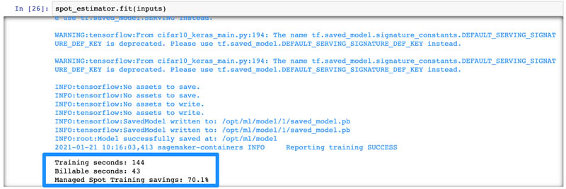
Towards the end of the job, you should see two lines of output:

• Training seconds: X – The actual compute time your training job spent
• Billable seconds: Y – The time you are billed for after Spot discounting is applied.

If you enabled use_spot_instances, you should see a notable difference between X and Y, signifying the cost savings you get for using Managed Spot Training. This is reflected in an additional line:

• Managed Spot Training savings – Calculated as (1-Y/X)*100 %

The following screenshot shows the output logs for our Jupyter notebook:

When the training is complete, you can also navigate to the Training jobs page on the SageMaker console and choose your training job to see how much you saved.

For this example training job of a model using TensorFlow, my training job ran for 144 seconds, but I’m only billed for 43 seconds, so for a 5 epoch training on a ml.p3.2xlarge GPU instance, I was able to save 70% on training cost!

Confirm that checkpoints and recovery works for when your training job is interrupted

How can you test if your training job will resume properly if a Spot Interruption occurs?

If you’re familiar with running EC2 Spot Instances, you know that you can simulate your application behavior during a Spot Interruption by following the recommended best practices. However, because SageMaker is a managed service, and manages the lifecycle of EC2 instances on your behalf, you can’t stop a SageMaker training instance manually. Your only option is to stop the entire training job.

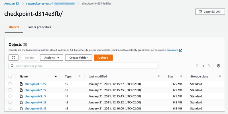
You can still test your code’s behavior when resuming an incomplete training by running a shorter training job, and then using the outputted checkpoints from that training job as inputs to a longer training job. To do this, first run a SageMaker Managed Spot Training job for a specified number of epochs as described in the previous section. Let’s say you run training for five epochs. SageMaker would have backed up your checkpoint files to the specified S3 location for the five epochs.

You can navigate to the training job details page on the SageMaker console to see the checkpoint configuration S3 output path.

Choose the S3 output path link to navigate to the checkpointing S3 bucket, and verify that five checkpoint files are available there.

Now run a second training run with 10 epochs. You should provide the first job’s checkpoint location to checkpoint_s3_uri so the training job can use those checkpoints as inputs to the second training job.

You can find the full implementation code in the GitHub repo.

The following is the relevant code:

hyperparameters = {'epochs': 10, 'batch-size': 256}

spot_estimator = TensorFlow(entry_point='cifar10_keras_main.py',
                       source_dir='source_dir',
                       metric_definitions=metric_definitions,
                       hyperparameters=hyperparameters,
                       role=role,
                       framework_version='1.15.2',
                       py_version='py3',
                       instance_count=1,
                       instance_type='ml.p3.2xlarge',
                       base_job_name='cifar10-tf-spot-2nd-run',
                       tags=tags,
                       checkpoint_s3_uri=checkpoint_s3_uri,
                       use_spot_instances=use_spot_instances,
                       max_run=max_run,
                       max_wait=max_wait)

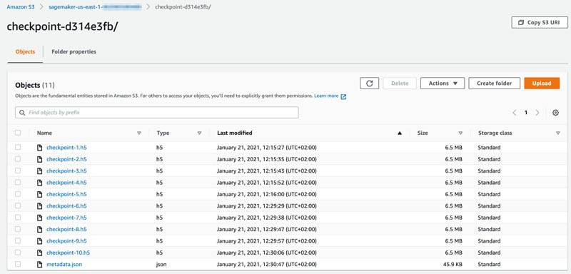
By providing checkpoint_s3_uri with your previous job’s checkpoints, you’re telling SageMaker to copy those checkpoints to your new job’s container. Your training script then loads the latest checkpoint and resumes training. The following screenshot shows that the training resumes resume from the sixth epoch.

To confirm that all checkpoint files were created, navigate to the same S3 bucket. This time you can see that 10 checkpoint files are available.

The key difference between simulating an interruption this way and how SageMaker manages interruptions is that you’re creating a new training job to test your code. In the case of Spot Interruptions, SageMaker simply resumes the existing interrupted job.

Implement checkpointing with PyTorch, MXNet, and XGBoost built-in and script mode

The steps shown in the TensorFlow example are basically the same for PyTorch and MXNet. The code for saving checkpoints and loading them to resume training is different.

You can see full examples for TensorFlow 1.x/2.x, PyTorch, MXNet, and XGBoost built-in and script mode in the GitHub repo.

Conclusions and next steps

In this post, we trained a TensorFlow image classification model using SageMaker Managed Spot Training. We saved checkpoints locally in the container and loaded checkpoints to resume training if they existed. SageMaker takes care of synchronizing the checkpoints with Amazon S3 and the training container. We simulated a Spot interruption by running Managed Spot Training with 5 epochs, and then ran a second Managed Spot Training Job with 10 epochs, configuring the checkpoints’ S3 bucket of the previous job. This resulted in the training job loading the checkpoints stored in Amazon S3 and resuming from the sixth epoch.

It’s easy to save on training costs with SageMaker Managed Spot Training. With minimal code changes, you too can save over 70% when training your deep-learning models.

As a next step, try to modify your own TensorFlow, PyTorch, or MXNet script to implement checkpointing, and then run a Managed Spot Training in SageMaker to see that the checkpoint files are created in the S3 bucket you specified. Let us know how you do in the comments!

About the Author

Eitan Sela is a Solutions Architect with Amazon Web Services. He works with AWS customers to provide guidance and technical assistance, helping them improve the value of their solutions when using AWS. Eitan also helps customers build and operate machine learning solutions on AWS. In his spare time, Eitan enjoys jogging and reading the latest machine learning articles.

Read More