 Face-off Probability is the National Hockey League’s (NHL) first advanced statistic using machine learning (ML) and artificial intelligence. It uses real-time Player and Puck Tracking (PPT) data to show viewers which player is likely to win a face-off before the puck is dropped, and provides broadcasters and viewers the opportunity to dive deeper into the importance of face-off matches and the differences in player abilities. Based on 10 years of historical data, hundreds of thousands of face-offs were used to engineer over 70 features fed into the model to provide real-time probabilities. Broadcasters can now discuss how a key face-off win by a player led to a goal or how the chances of winning a face-off decrease as a team’s face-off specialist is waived out of a draw. Fans can see visual, real-time predictions that show them the importance of a key part of the game.
In this post, we focus on how the ML model for Face-off Probability was developed and the services used to put the model into production. We also share the key technical challenges that were solved during construction of the Face-off Probability model.
How it works
Imagine the following scenario: It’s a tie game between two NHL teams that will determine who moves forward. We’re in the third period with 1:22 seconds left to play. Two players from opposite teams line up to take the draw in the closest face-off closer to one of the nets. The linesman notices a defensive player encroaching into the face-off circle and waives their player out of the face-off due to the violation. A less experienced defensive player comes in to take the draw as his replacement. The attacking team wins the face-off, gets possession of the puck, and immediately scores to take the lead. The score holds up for the remaining minute of the game and decides who moves forward. What player was favored to win the face-off before the initial duo was changed? How much did the defensive’s team probability of winning the face-off decrease by the violation that forced a different player to take the draw? Face-off Probability, the newest NHL Edge IQ statistic powered by AWS, can now answer these questions.
When there is a stoppage in play, Face-off Probability generates predictions for who will win the upcoming face-off based on the players on the ice, the location of the face-off, and the current game situation. The predictions are generated throughout the stoppage until the game clock starts running again. Predictions occur at sub-second latency and are triggered any time there is a change in the players involved in the face-off.

Overcoming key obstacles for face-off probability
Predicting face-off probability in real-time broadcasts can be broken down into two specific sub-problems:
- Modeling the face-off event as an ML problem, understanding the requirements and limitations, preparing the data, engineering the data signals, exploring algorithms, and ensuring reliability of results
- Detecting a face-off event during the game from a stream of PPT events, collecting parameters needed for prediction, calling the model, and submitting results to broadcasters
Predicting the probability of a player winning a face-off in real time on a televised broadcast has several technical challenges that had to be overcome. These included determining the features required and modeling methods to predict an event that has a large amount of uncertainty, and determining how to use streaming PPT sensor data to identify where a face-off is occurring, the players involved, and the probability of each player winning the face-off, all within hundreds of milliseconds.

Building an ML model for difficult-to-predict events
Predicting events such as face-off winning probabilities during a live game is a complex task that requires a significant amount of quality historic data and data streaming capabilities. To identify and understand the important signals in such a rich data environment, the development of ML models requires extensive subject matter expertise. The Amazon Machine Learning Solutions Lab partnered with NHL hockey and data experts to work backward from their target goal of enhancing their fan experience. By continuously listening to NHL’s expertise and testing hypotheses, AWS’s scientists engineered over 100 features that correlate to the face-off event. In particular, the team classified this feature set into one of three categories:
- Historical statistics on player performances such as the number of face-offs a player has taken and won in the last five seasons, the number of face-offs the player has taken and won in previous games, a player’s winning percentages over several time windows, and the head-to-head winning percentage for each player in the face-off
- Player characteristics such as height, weight, handedness, and years in the league
- In-game situational data that might affect a player’s performance, such as the score of the game, the elapsed time in the game to that point, where the face-off is located, the strength of each team, and which player has to put their stick down for the face-off first
AWS’s ML scientists considered the problem as a binary classification problem: either the home player wins the face-off or the away player wins the face-off. With data from more than 200,000 historical face-offs, they used a LightGBM model to predict which of the two players involved with a face-off event is likely to win.
Determining if a face-off is about to occur and which players are involved
When a whistle blows and the play is stopped, Face-off Probability begins to make predictions. However, Face-off Probability has to first determine where the face-off is occurring and which player from each team is involved in the face-off. The data stream indicates events as they occur but doesn’t provide information on when an event is likely to occur in the future. As such, the sensor data of the players on the ice is needed to determineif and where a face-off is about to happen.
The PPT system produces real-time locations and velocities for players on the ice at up to 60 events per second. These locations and velocities were used to determine where the face-off is happening on the ice and if it’s likely to happen soon. By knowing how close the players are to known face-off locations and how stationary the players were, Face-off Probability was able to determine that a face-off was likely to occur and the two players that would be involved in the face-off.
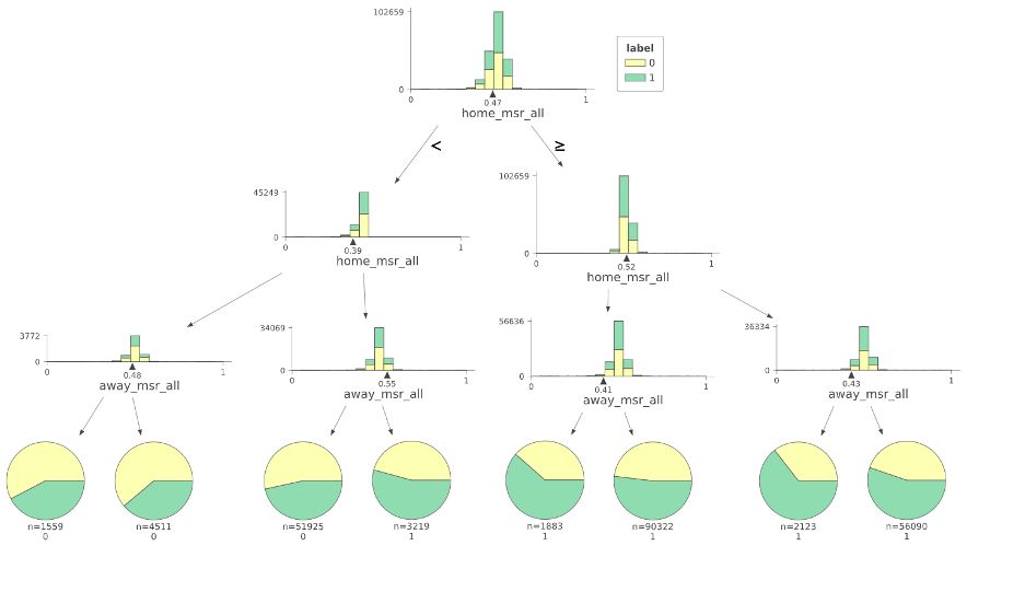
Determining the correct cut-off distance for proximity to a face-off location and the corresponding cut-off velocity for stationary players was accomplished using a decision tree model. With PPT data from the 2020-2021 season, we built a model to predict the likelihood that a face-off is occurring at a specified location given the average distance of each team to the location and the velocities of the players. The decision tree provided the cut-offs for each metric, which we included as rules-based logic in the streaming application.
With the correct face-off location determined, the player from each team taking the face-off was calculated by taking the player closest to the known location from each team. This provided the application with the flexibility to identify the correct players while also being able to adjust to a new player having to take a face-off if a current player is waived out due to an infraction. Making and updating the prediction for the correct player was a key focus for the real-time usability of the model in broadcasts, which we describe further in the next section.
Model development and training
To develop the model, we used more than 200,000 historical face-off data points, along with the custom engineered feature set designed by working with the subject matter experts. We looked at features like in-game situations, historical performance of the players taking the face-off, player-specific characteristics, and head-to-head performances of the players taking the face-off, both in the current season and for their careers. Collectively, this resulted in over 100 features created using a combination of available and derived techniques.
To assess different features and how they might influence the model, we conducted extensive feature analysis as part of the exploratory phase. We used a mix of univariate tests and multivariate tests. For multivariate tests, for interpretability, we used decision tree visualization techniques. To assess statistical significance, we used Chi Test and KS tests to test dependence or distribution differences.
We explored classification techniques and models with the expectation that the raw probabilities would be treated as the predictions. We explored nearest neighbors, decision trees, neural networks, and also collaborative filtering in terms of algorithms, while trying different sampling strategies (filtering, random, stratified, and time-based sampling) and evaluated performance on Area Under the Curve (AUC) and calibration distribution along with Brier score loss. At the end, we found that the LightGBM model worked best with well-calibrated accuracy metrics.
To evaluate the performance of the models, we used multiple techniques. We used a test set that the trained model was never exposed to. Additionally, the teams conducted extensive manual assessments of the results, looking at edge cases and trying to understand the nuances of how the model looked to determine why a certain player should have won or lost a face-off event.
With information collected from manual reviewers, we would adjust the features when required, or run iterations on the model to see if the performance of the model was as expected.
Deploying Face-off Probability for real-time use during national television broadcasts
One of the goals of the project was not just to predict the winner of the face-off, but to build a foundation for solving a number of similar problems in a real-time and cost-efficient way. That goal helped determine which components to use in the final architecture.
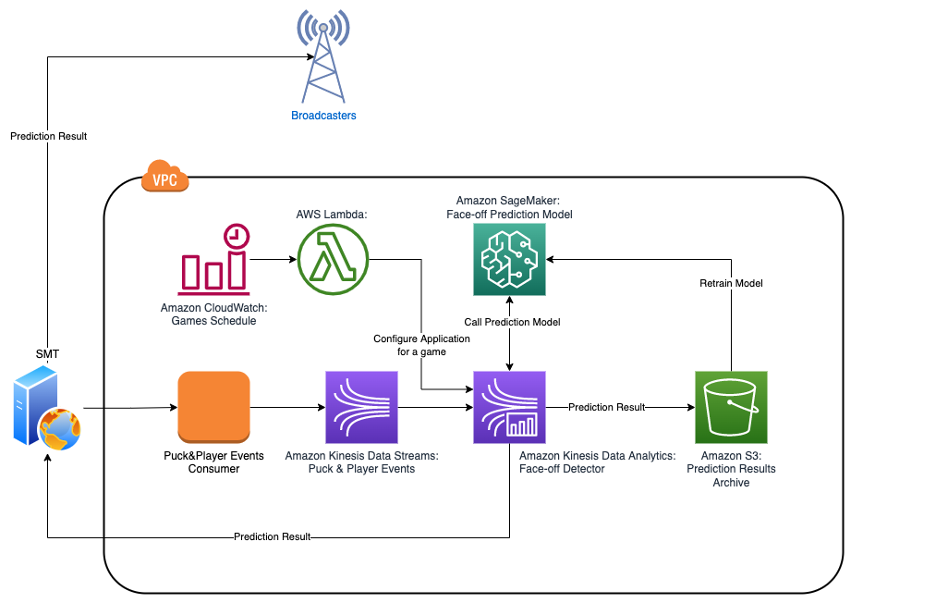
The first important component is Amazon Kinesis Data Streams, a serverless streaming data service that acts as a decoupler between the specific implementation of the PPT data provider and consuming applications, thereby protecting the latter from the disrupting changes in the former. It has also enhanced the fan-out feature, which provides the ability to connect up to 20 parallel consumers and maintain a low latency of 70 milliseconds and the same throughput of 2MB/s per shard between all of them simultaneously.
PPT events don’t come for all players at once, but arrive discretely for each player as well as other events in the game. Therefore, to implement the upcoming face-off detection algorithm, the application needs to maintain a state.
The second important component of the architecture is Amazon Kinesis Data Analytics for Apache Flink. Apache Flink is a distributed streaming, high-throughput, low-latency data flow engine that provides a convenient and easy way to use the Data Stream API, and it supports stateful processing functions, checkpointing, and parallel processing out of the box. This helps speed up development and provides access to low-level routines and components, which allows for a flexible design and implementation of applications.
Kinesis Data Analytics provides the underlying infrastructure for your Apache Flink applications. It eliminates a need to deploy and configure a Flink cluster on Amazon Elastic Compute Cloud (Amazon EC2) or Kubernetes, which reduces maintenance complexity and costs.
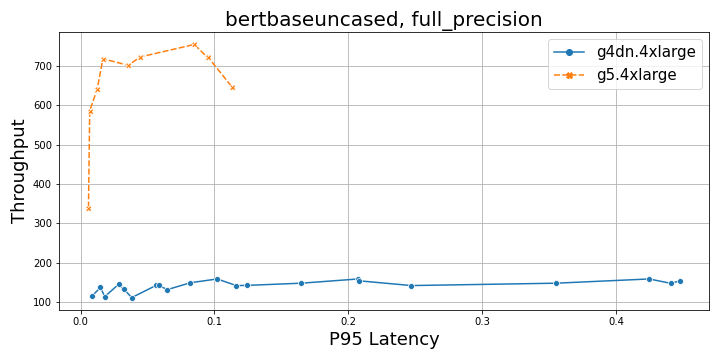
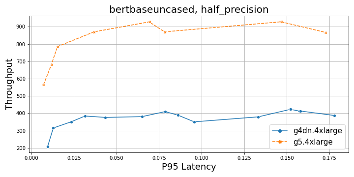
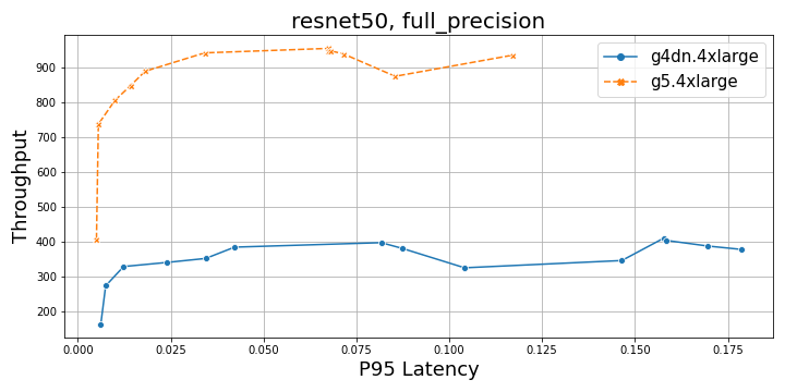
The third crucial component is Amazon SageMaker. Although we used SageMaker to build a model, we also needed to make a decision at the early stages of the project: should scoring be implemented inside the face-off detecting application itself and complicate the implementation, or should the face-off detecting application call SageMaker remotely and sacrifice some latency due to communication over the network? To make an informed decision, we performed a series of benchmarks to verify SageMaker latency and scalability, and validated that average latency was less than 100 milliseconds under the load, which was within our expectations.
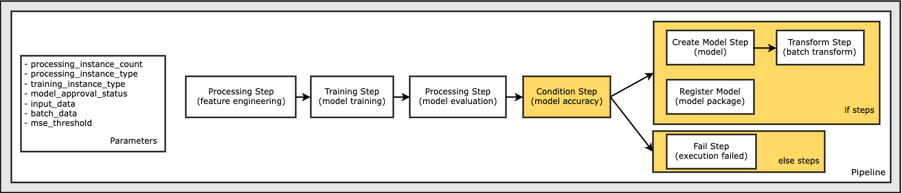
With the main parts of high-level architecture decided, we started to work on the internal design of the face-off detecting application. A computation model of the application is depicted in the following diagram.

The compute model of the face-off detecting application can be modeled as a simple finite-state machine, where each incoming message transitions the system from one state to another while performing some computation along with that transition. The application maintains several data structures to keep track of the following:
- Changes in the game state – The current period number, status and value of the game clock, and score
- Changes in the player’s state – If the player is currently on the ice or on the bench, the current coordinates on the field, and the current velocity
- Changes in the player’s personal face-off stats – The success rate of one player vs. another, and so on
The algorithm checks each location update event of a player to decide whether a face-off prediction should be made and whether the result should be submitted to broadcasters. Taking into account that each player location is updated roughly every 80 milliseconds and players move much slower during game pauses than during the game, we can conclude that the situation between two updates doesn’t drastically change. If the application called SageMaker for predictions and sent predictions to broadcasters every time a new location update event was received and all conditions are satisfied, SageMaker and the broadcasters would be overwhelmed with a number of duplicate requests.
To avoid all this unnecessary noise, the application keeps track of a combination of parameters for which predictions were already made, along with the result of the prediction, and caches them in memory to avoid expensive duplicate requests to SageMaker. Also, it keeps track of what predictions were already sent to broadcasters and makes sure that only new predictions are sent or the previously sent ones are sent again only if necessary. Testing showed that this approach reduces the amount of outgoing traffic by more than 100 times.
Another optimization technique that we used was grouping requests to SageMaker and performing them asynchronously in parallel. For example, if we have four new combinations of face-off parameters for which we need to get predictions from SageMaker, we know that each request will take less than 100 milliseconds. If we perform each request synchronously one by one, the total response time will be under 400 milliseconds. But if we group all four requests, submit them asynchronously, and wait for the result for the entire group before moving forward, we effectively parallelize requests and the total response time will be under 100 milliseconds, just like for only one request.
Summary
NHL Edge IQ, powered by AWS, is bringing fans closer to the action with advanced analytics and new ML stats. In this post, we showed insights into the building and deployment of the new Face-off Probability model, the first on-air ML statistic for the NHL. Be sure to keep an eye out for the probabilities generated by Face-off Probability in upcoming NHL games.
To find full examples of building custom training jobs for SageMaker, visit Bring your own training-completed model with SageMaker by building a custom container. For examples of using Amazon Kinesis for streaming, refer to Learning Amazon Kinesis Development.
To learn more about the partnership between AWS and the NHL, visit NHL Innovates with AWS Cloud Services. If you’d like to collaborate with experts to bring ML solutions to your organization, contact the Amazon ML Solutions Lab.
About the Authors
 Ryan Gillespie is a Sr. Data Scientist with AWS Professional Services. He has a MSc from Northwestern University and a MBA from the University of Toronto. He has previous experience in the retail and mining industries.
 Yash Shah is a Science Manager in the Amazon ML Solutions Lab. He and his team of applied scientists and machine learning engineers work on a range of machine learning use cases from healthcare, sports, automotive and manufacturing.
 Alexander Egorov is a Principal Data Architect, specializing in streaming technologies. He helps organizations to design and build platforms for processing and analyzing streaming data in real time.
 Miguel Romero Calvo is an Applied Scientist at the Amazon ML Solutions Lab where he partners with AWS internal teams and strategic customers to accelerate their business through ML and cloud adoption.
 Erick Martinez is a Sr. Media Application Architect with 25+ years of experience, with focus on Media and Entertainment. He is experienced in all aspects of systems development life-cycle ranging from discovery, requirements gathering, design, implementation, testing, deployment, and operation.


 Paul Hargis has focused his efforts on machine learning at several companies, including AWS, Amazon, and Hortonworks. He enjoys building technology solutions and teaching people how to make the most of it. Prior to his role at AWS, he was lead architect for Amazon Exports and Expansions, helping amazon.com improve the experience for international shoppers. Paul likes to help customers expand their machine learning initiatives to solve real-world problems.
 Niklas Palm is a Solutions Architect at AWS in Stockholm, Sweden, where he helps customers across the Nordics succeed in the cloud. He’s particularly passionate about serverless technologies along with IoT and machine learning. Outside of work, Niklas is an avid cross-country skier and snowboarder as well as a master egg boiler.
 Kirit Thadaka is an ML Solutions Architect working in the SageMaker Service SA team. Prior to joining AWS, Kirit worked in early-stage AI startups followed by some time consulting in various roles in AI research, MLOps, and technical leadership.


 Bosco Albuquerque is a Sr. Partner Solutions Architect at AWS and has over 20 years of experience working with database and analytics products from enterprise database vendors and cloud providers. He has helped technology companies design and implement data analytics solutions and products.
 Frank Dallezotte is a Sr. Solutions Architect at AWS and is passionate about working with independent software vendors to design and build scalable applications on AWS. He has experience creating software, implementing build pipelines, and deploying these solutions in the cloud.
 Charles Laughlin is a Principal AI/ML Specialist Solutions Architect and works on the Time Series ML team at AWS. He helps shape the Amazon Forecast service roadmap and collaborates daily with diverse AWS customers to help transform their businesses using cutting-edge AWS technologies and thought leadership. Charles holds an M.S. in Supply Chain Management and has spent the past decade working in the consumer packaged goods industry.
 James Sun is a Senior Partner Solutions Architect at Snowflake. James has over 20 years of experience in storage and data analytics. Prior to Snowflake, he held several senior technical positions at AWS and MapR. James holds a PhD from Stanford University.


 Amr Ragab is a Principal Solutions Architect for EC2 Accelerated Platforms for AWS, devoted to helping customers run computational workloads at scale. In his spare time he likes traveling and finding new ways to integrate technology into daily life.