Amazon Neptune ML is a machine learning (ML) capability of Amazon Neptune that helps you make accurate and fast predictions on your graph data. Under the hood, Neptune ML uses Graph Neural Networks (GNNs) to simultaneously take advantage of graph structure and node/edge properties to solve the task at hand. Traditional methods either only use properties and no graph structure (e.g., XGBoost, Neural Networks), or only graph structure and no properties (e.g., node2vec, Label Propagation). To better manipulate the node/edge properties, ML algorithms require the data to be well behaved numerical data, but raw data in a database can have other types, like raw text. To make use of these other types of data, we need specialized processing steps that convert them from their native type into numerical data, and the quality of the ML results is strongly dependent on the quality of these data transformations. Raw text, like sentences, are among the most difficult types to transform, but recent progress in the field of Natural Language Processing (NLP) has led to strong methods that can handle text coming from multiple languages and a wide variety of lengths.
Beginning with version 1.1.0.0, Neptune ML supports multiple text encoders (text_fasttext, text_sbert, text_word2vec, and text_tfidf), which bring the benefits of recent advances in NLP and enables support for multi-lingual text properties as well as additional inference requirements around languages and text length. For example, in a job recommendation use case, the job posts in different countries can be described in different languages and the length of job descriptions vary considerably. Additionally, Neptune ML supports an auto option that automatically chooses the best encoding method based on the characteristics of the text feature in the data.
In this post, we illustrate the usage of each text encoder, compare their advantages and disadvantages, and show an example of how to choose the right text encoders for a job recommendation task.
What is a text encoder?
The goal of text encoding is to convert the text-based edge/node properties in Neptune into fixed-size vectors for use in downstream machine learning models for either node classification or link prediction tasks. The length of the text feature can vary a lot. It can be a word, phrase, sentence, paragraph, or even a document with multiple sentences (the maximum size of a single property is 55 MB in Neptune). Additionally, the text features can be in different languages. There may also be sentences that contain words in several different languages, which we define as code-switching.
Beginning with the 1.1.0.0 release, Neptune ML allows you to choose from several different text encoders. Each encoder works slightly differently, but has the same goal of converting a text value field from Neptune into a fixed-size vector that we use to build our GNN model using Neptune ML. The new encoders are as follows:
-
text_fasttext (new) – Uses fastText encoding. FastText is a library for efficient text representation learning.
text_fasttextis recommended for features that use one and only one of the five languages that fastText supports (English, Chinese, Hindi, Spanish, and French). Thetext_fasttextmethod can optionally take themax_lengthfield, which specifies the maximum number of tokens in a text property value that will be encoded, after which the string is truncated. You can regard a token as a word. This can improve performance when text property values contain long strings, because ifmax_lengthis not specified, fastText encodes all the tokens regardless of the string length. -
text_sbert (new) – Uses the Sentence BERT (SBERT) encoding method. SBERT is a kind of sentence embedding method using the contextual representation learning models, BERT-Networks.
text_sbertis recommended when the language is not supported bytext_fasttext. Neptune supports two SBERT methods:text_sbert128, which is the default if you just specifytext_sbert, andtext_sbert512. The difference between them is the maximum number of tokens in a text property that get encoded. Thetext_sbert128encoding only encodes the first 128 tokens, whereastext_sbert512encodes up to 512 tokens. As a result, usingtext_sbert512can require more processing time thantext_sbert128. Both methods are slower thantext_fasttext. - text_word2vec – Uses Word2Vec algorithms originally published by Google to encode text. Word2Vec only supports English.
- text_tfidf – Uses a term frequency-inverse document frequency (TF-IDF) vectorizer for encoding text. TF-IDF encoding supports statistical features that the other encodings do not. It quantifies the importance or relevance of words in one node property among all the other nodes.
Note that text_word2vec and text_tfidf were previously supported and the new methods text_fasttext and text_sbert are recommended over the old methods.
Comparison of different text encoders
The following table shows the detailed comparison of all the supported text encoding options (text_fasttext, text_sbert, and text_word2vec). text_tfidf is not a model-based encoding method, but rather a count-based measure that evaluates how relevant a token (for example, a word) is to the text features in other nodes or edges, so we don’t include text_tfidf for comparison. We recommend using text_tfidf when you want to quantify the importance or relevance of some words in one node or edge property amongst all the other node or edge properties.)
| . | . | text_fasttext | text_sbert | text_word2vec |
| Model Capability | Supported language | English, Chinese, Hindi, Spanish, and French | More than 50 languages | English |
| Can encode text properties that contain words in different languages | No | Yes | No | |
| Max-length support | No maximum length limit | Encodes the text sequence with the maximum length of 128 and 512 | No maximum length limit | |
| Time Cost | Loading | Approximately 10 seconds | Approximately 2 seconds | Approximately 2 seconds |
| Inference | Fast | Slow | Medium |
Note the following usage tips:
- For text property values in English, Chinese, Hindi, Spanish, and French,
text_fasttextis the recommended encoding. However, it can’t handle cases where the same sentence contains words in more than one language. For other languages than the five thatfastTextsupports, usetext_sbertencoding. - If you have many property value text strings longer than, for example, 120 tokens, use the
max_lengthfield to limit the number of tokens in each string thattext_fasttextencodes.
To summarize, depending on your use case, we recommend the following encoding method:
- If your text properties are in one of the five supported languages, we recommend using
text_fasttextdue to its fast inference.text_fasttextis the recommended choices and you can also usetext_sbertin the following two exceptions. - If your text properties are in different languages, we recommend using
text_sbertbecause it’s the only supported method that can encode text properties containing words in several different languages. - If your text properties are in one language that isn’t one of the five supported languages, we recommend using
text_sbertbecause it supports more than 50 languages. - If the average length of your text properties is longer than 128, consider using
text_sbert512ortext_fasttext. Both methods can use encode longer text sequences. - If your text properties are in English only, you can use
text_word2vec, but we recommend usingtext_fasttextfor its fast inference.
Use case demo: Job recommendation task
The goal of the job recommendation task is to predict what jobs users will apply for based on their previous applications, demographic information, and work history. This post uses an open Kaggle dataset. We construct the dataset as a three-node type graph: job, user, and city.

A job is characterized by its title, description, requirements, located city, and state. A user is described with the properties of major, degree type, number of work history, total number of years for working experience, and more. For this use case, job title, job description, job requirements, and majors are all in the form of text.
In the dataset, users have the following properties:
- State – For example, CA or 广东省 (Chinese)
- Major – For example, Human Resources Management or Lic Cytura Fisica (Spanish)
- DegreeType – For example, Bachelor’s, Master’s, PhD, or None
- WorkHistoryCount – For example, 0, 1, 16, and so on
- TotalYearsExperience – For example, 0.0, 10.0, or NAN
Jobs have the following properties:
- Title – For example, Administrative Assistant or Lic Cultura Física (Spanish).
- Description – For example, “This Administrative Assistant position is responsible for performing a variety of clerical and administrative support functions in the areas of communications, …” The average number of words in a description is around 192.2.
- Requirements – For example, “JOB REQUIREMENTS: 1. Attention to detail; 2.Ability to work in a fast paced environment;3.Invoicing…”
- State: – For example, CA, NY, and so on.
The node type city like Washington DC and Orlando FL only has the identifier for each node. In the following section, we analyze the characteristics of different text features and illustrate how to select the proper text encoders for different text properties.
How to select different text encoders
For our example, the Major and Title properties are in multiple languages and have short text sequences, so text_sbert is recommended. The sample code for the export parameters is as follows. For the text_sbert type, there are no other parameter fields. Here we choose text_sbert128 other than text_sbert512, because the text length is relatively shorter than 128.
The Description and Requirements properties are usually in long text sequences. The average length of a description is around 192 words, which is longer than the maximum input length of text_sbert (128). We can use text_sbert512, but it may result in slower inference. In addition, the text is in a single language (English). Therefore, we recommend text_fasttext with the en language value because of its fast inference and not limited input length. The sample code for the export parameters is as follows. The text_fasttext encoding can be customized using language and max_length. The language value is required, but max_length is optional.
More details of the job recommendation use cases can be found in the Neptune notebook tutorial.
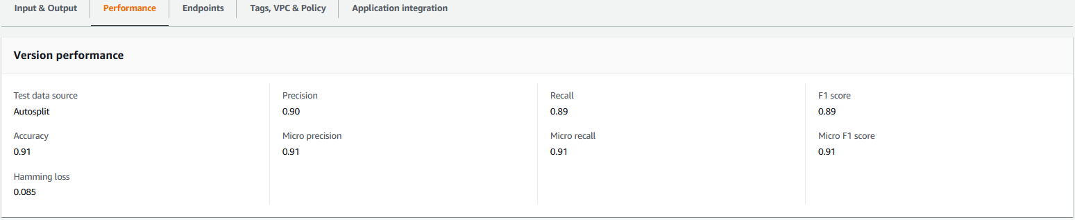
For demonstration purposes, we select one user, i.e., user 443931, who holds a Master’s degree in ‘Management and Human Resources. The user has applied to five different jobs, titled as “Human Resources (HR) Manager”, “HR Generalist”, “Human Resources Manager”, “Human Resources Administrator”, and “Senior Payroll Specialist”. In order to evaluate the performance of the recommendation task, we delete 50% of the apply jobs (the edges) of the user (here we delete “Human Resources Administrator” and “Human Resources (HR) Manager) and try to predict the top 10 jobs this user is most likely to apply for.
After encoding the job features and user features, we perform a link prediction task by training a relational graph convolutional network (RGCN) model. Training a Neptune ML model requires three steps: data processing, model training, and endpoint creation. After the inference endpoint has been created, we can make recommendations for user 443931. From the predicted top 10 jobs for user 443931 (i.e., “HR Generalist”, “Human Resources (HR) Manager”, “Senior Payroll Specialist”, “Human Resources Administrator”, “HR Analyst”, et al.), we observe that the two deleted jobs are among the 10 predictions.
Conclusion
In this post, we showed the usage of the newly supported text encoders in Neptune ML. These text encoders are simple to use and can support multiple requirements. In summary,
- text_fasttext is recommended for features that use one and only one of the five languages that text_fasttext supports.
- text_sbert is recommended for text that text_fasttext doesn’t support.
- text_word2vec only supports English, and can be replaced by text_fasttext in any scenario.
For more details about the solution, see the GitHub repo. We recommend using the text encoders on your graph data to meet your requirements. You can just choose an encoder name and set some encoder attributes, while keeping the GNN model unchanged.
About the authors
 Jiani Zhang is an applied scientist of AWS AI Research and Education (AIRE). She works on solving real-world applications using machine learning algorithms, especially natural language and graph related problems.


 Sofian Hamiti is an AI/ML specialist Solutions Architect at AWS. He helps customers across industries accelerate their AI/ML journey by helping them build and operationalize end-to-end machine learning solutions.
 Dr. Romi Datta is a Senior Manager of Product Management in the Amazon SageMaker team responsible for training, processing and feature store. He has been in AWS for over 4 years, holding several product management leadership roles in SageMaker, S3 and IoT. Prior to AWS he worked in various product management, engineering and operational leadership roles at IBM, Texas Instruments and Nvidia. He has an M.S. and Ph.D. in Electrical and Computer Engineering from the University of Texas at Austin, and an MBA from the University of Chicago Booth School of Business.


 Lana Zhang is a Sr. Solutions Architect at the AWS WWSO AI Services team with expertise in AI and ML for intelligent document processing and content moderation. She is passionate about promoting AWS AI services and helping customers transform their business solutions.