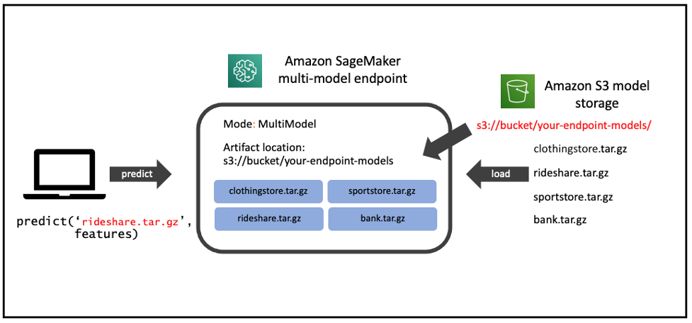
HawkEye 360 uses Amazon SageMaker Autopilot to streamline machine learning model development for maritime vessel risk assessment

This post is cowritten by Ian Avilez and Tim Pavlick from HawkEye 360.

HawkEye 360 is a commercial radio frequency (RF) satellite constellation data analytics provider. Our signals of interest include very high frequency (VHF) push-to-talk radios, maritime radar systems, AIS beacons, satellite mobile comms, and more. Our Mission Space offering, released in February 2021, allows mission analysts to intuitively visualize RF signals and analytics, which allows them to identify activity and understand trends. This capability improves maritime situational awareness for mission analysts, allowing them to identify and characterize nefarious behavior such as illegal fishing or ship-to-ship transfer of illicit goods.

The following screenshot shows HawkEye 360’s Mission Space experience.

RF data can be overwhelming to the naked eye without filtering and advanced algorithms to parse through and characterize the vast amount of raw data. HawkEye 360 partnered with the Amazon ML Solutions Lab to build machine learning (ML) capabilities into our analytics. With the guidance of the Amazon ML Solutions Lab, we used Amazon SageMaker Autopilot to rapidly generate high-quality AI models for maritime vessel risk assessment, maintain full visibility and control of model creation, and provide the ability to easily deploy and monitor a model in a production environment.

Hidden patterns and relationships among vessel features

Seagoing vessels are distinguished by several characteristics relating to the vessel itself, its operation and management, and its historical behavior. Knowing which characteristics are indicative of a suspicious vessel isn’t immediately clear. One of HawkEye 360’s missions is to discover hidden patterns and automatically alert analysts to anomalous maritime activity. Hawkeye 360 accomplishes this alerting regions by using a diverse set of variables, in combination with proprietary RF geo-analytics. A key focus of these efforts is to identify which vessels are more likely to engage in suspicious maritime activity, such as illegal fishing or ship-to-ship transfer of illicit goods. ML algorithms reveal hidden patterns, where they exist, that would otherwise be lost in the vast sea of complexity.

The following image demonstrates some of the existing pattern finding behavior that has been built into Mission Space. Mission Space automatically identifies other instances of a suspicious vessel. Identifying the key features, that are most predictive of suspicious behavior, allows for easy display of those features in Mission Space. This enables users to understand links between bad actors that would otherwise have never been seen. Mission Space was purposefully designed to point out these connections to mission analysts.

The following image demonstrates some of the existing pattern finding behavior that has been built into Mission Space.

Challenges detecting anomalous behavior with maritime vessels

HawkEye 360’s data lake includes a large volume of vessel information, history, and analytics variables. With such a wide array of RF data and analytics, some natural data handling issues must be addressed. Sporadic reporting by vessels results in missing values across datasets. Variations amongst data types must be taken into account. Previously, data exploration and baseline modeling typically would takes up a large chunk of an analysts’ time. After the data is prepared, a series of automatic experiments is run to narrow down to a set of the most promising AI models, and in a stepwise fashion from there, to select the one most appropriate for the data and the research questions. For HawkEye 360, this automated exploration is key to determining which features, and feature combinations, are critical to predicting how likely a vessel is to engage in suspicious behavior.

We used Autopilot to expedite this process by quickly identifying which features of the data are useful in predicting suspicious behavior. Automation of data exploration and analysis enables our data scientists to spend less time wrangling data and manually engineering features, and expedites the ability to identify the vessel features that are most predictive of suspicious vessel behavior.

How we used Autopilot to quickly generate high-quality ML models

As part of an Autopilot job, several candidate models are generated rapidly for evaluation with a single API call. Autopilot inspected the data and evaluated several models to determine the optimal combination of preprocessing methods, ML algorithms, and hyperparameters. This significantly shortened the model exploration time frame and allowed us to quickly test the suitability of ML to our unique hypotheses.

The following code shows our setup and API call:

input_data_config = [{
      'DataSource': {
        'S3DataSource': {
          'S3DataType': 'S3Prefix',
          'S3Uri': 's3://{}/{}/train'.format(bucket,prefix)
        }
      },
      'TargetAttributeName': 'ship_sanctioned_ofac'
    }
  ]

output_data_config = {
    'S3OutputPath': 's3://{}/{}/output'.format(bucket,prefix)
  }

from time import gmtime, strftime, sleep
timestamp_suffix = strftime('%d-%H-%M-%S', gmtime())

auto_ml_job_name = 'automl-darkcount-' + timestamp_suffix
print('AutoMLJobName: ' + auto_ml_job_name)

sm.create_auto_ml_job(AutoMLJobName=auto_ml_job_name,
                      InputDataConfig=input_data_config,
                      OutputDataConfig=output_data_config,
                      RoleArn=role)

Autopilot job process

An Autopilot job consists of the following actions:

  • Dividing the data into train and validation sets
  • Analyzing the data to recommend candidate configuration
  • Performing feature engineering to generate optimal transformed features appropriate for the algorithm
  • Tuning hyperparameters to generate a leaderboard of models
  • Surfacing the best candidate model based on the given evaluation metric

After we trained several models, Autopilot racks and stacks the trained candidates based on a given metric (see the following code). For this application, we used an F1 score, which gives an even weight to both precision and recall. This is an important consideration when classes are imbalanced, which they are in this dataset.

candidates = sm.list_candidates_for_auto_ml_job(AutoMLJobName=auto_ml_job_name, SortBy='FinalObjectiveMetricValue')['Candidates']
index = 1
print("List of model candidates in descending objective metric:")
for candidate in candidates:
    print (str(index) + "  " + candidate['CandidateName'] + "  " + str(candidate['FinalAutoMLJobObjectiveMetric']['Value']))
    index += 1

The following code shows our output:

List of model candidates in descending objective metric:

1 tuning-job-1-1be4d5a5fb8e42bc84-238-e264d09f 0.9641900062561035
2 tuning-job-1-1be4d5a5fb8e42bc84-163-336eb2e7 0.9641900062561035
3 tuning-job-1-1be4d5a5fb8e42bc84-143-5007f7dc 0.9641900062561035
4 tuning-job-1-1be4d5a5fb8e42bc84-154-cab67dc4 0.9641900062561035
5 tuning-job-1-1be4d5a5fb8e42bc84-123-f76ad56c 0.9641900062561035
6 tuning-job-1-1be4d5a5fb8e42bc84-117-39eac182 0.9633200168609619
7 tuning-job-1-1be4d5a5fb8e42bc84-108-77addf80 0.9633200168609619
8 tuning-job-1-1be4d5a5fb8e42bc84-179-1f831078 0.9633200168609619
9 tuning-job-1-1be4d5a5fb8e42bc84-133-917ccdf1 0.9633200168609619
10 tuning-job-1-1be4d5a5fb8e42bc84-189-102070d9 0.9633200168609619

We can now create a model from the best candidate, which can be quickly deployed into production:

model_name = 'automl-darkcount-25-23-07-39'

model = sm.create_model(Containers=best_candidate['InferenceContainers'],
                            ModelName=model_name,
                            ExecutionRoleArn=role)

print('Model ARN corresponding to the best candidate is : {}'.format(model['ModelArn']))

The following code shows our output:

Model ARN corresponding to the best candidate is : arn:aws:sagemaker:us-east-1:278150328949:model/automl-darkcount-25-23-07-39

Maintaining full visibility and control

The process to generate a model is completely transparent. Two notebooks are generated for any model Autopilot creates:

  • Data exploration notebook – Describes your dataset and what Autopilot learned about your dataset
  • Model candidate notebook – Lists data transformations used as well as candidate model building pipelines consisting of feature transformers paired with main estimators

Conclusion

We used Autopilot to quickly generate many candidate models to determine ML feasibility and baselining ML performance on the vessel data. The automaticity of Autopilot allowed our data scientists to spend 50% less time developing ML capabilities by automating the manual tasks such as data analysis, feature engineering, model development, and model deployment.

With HawkEye 360’s new RF data analysis application, Mission Space, identifying which vessels have the potential to engage in suspicious activity allows users to easily know where to focus their scarce attention and investigate further. Expediting the data understanding and model creation allows for cutting-edge insights to be quickly assimilated into Mission Space, which accelerates the evolution of Mission Space’s capabilities as shown in the following map. We can see that a Mission Analyst identified a specific rendezvous (highlighted in magenta) and Mission Space automatically identified other related rendezvous (in purple).

For example, in the following map, we can see Mission Space identified a specific rendezvous

For more information about HawkEye 360’s Mission Space offering, see Misson Space.

If you’d like assistance in accelerating the use of ML in your products and services, contact the Amazon ML Solutions Lab.


About the Authors

  Tim Pavlick, PhD, is VP of Product at HawkEye 360. He is responsible for the conception, creation, and productization of all HawkEye space innovations. Mission Space is HawkEye 360’s flagship product, incorporating all the data and analytics from the HawkEye portfolio into one intuitive RF experience. Dr. Pavlick’s prior invention contributions include Myca, IBM’s AI Career Coach, Grit PTSD monitor for Veterans, IBM Defense Operations Platform, Smarter Planet Intelligent Operations Center, AI detection of dangerous hate speech on the internet, and the STORES electronic food ordering system for the US military. Dr. Pavlick received his PhD in Cognitive Psychology from the University of Maryland College Park.

Ian Avilez is a Data Scientist with HawkEye 360. He works with customers to highlight the insights that can be gained by combining different datasets and looking at that data in various ways.


Dan Ford is a Data Scientist at the Amazon ML Solution Lab, where he helps AWS National Security customers build state-of-the-art ML solutions.


Gaurav Rele is a Data Scientist at the Amazon ML Solution Lab, where he works with AWS customers across different verticals to accelerate their use of machine learning and AWS Cloud services to solve their business challenges.

Read More

Protecting people from hazardous areas through virtual boundaries with Computer Vision

As companies welcome more autonomous robots and other heavy equipment into the workplace, we need to ensure equipment can operate safely around human teammates. In this post, we will show you how to build a virtual boundary with computer vision and AWS DeepLens, the AWS deep learning-enabled video camera designed for developers to learn machine learning (ML). Using the machine learning techniques in this post, you can build virtual boundaries for restricted areas that automatically shut down equipment or sound an alert when humans come close.

For this project, you will train a custom object detection model with Amazon SageMaker and deploy the model to an AWS DeepLens device. Object detection is an ML algorithm that takes an image as input and identifies objects and their location within the image. In addition to virtual boundary solutions, you can apply techniques learned in this post when you need to detect where certain objects are inside an image or count the number of instances of a desired object in an image, such as counting items in a storage bin or on a retail shelf.

Solution overview

The walkthrough includes the following steps:

  1. Prepare your dataset to feed into an ML algorithm.
  2. Train a model with Amazon SageMaker.
  3. Test model with custom restriction zones.
  4. Deploy the solution to AWS DeepLens.

We also discuss other real-world use cases where you can apply this solution.

The following diagram illustrates the solution architecture.

Prerequisites

To complete this walkthrough, you must have the following prerequisites:

Prepare your dataset to feed into an ML algorithm

This post uses an ML algorithm called an object detection model to build a solution that detects if a person is in a custom restricted zone. You use the publicly available Pedestrian Detection dataset available on Kaggle, which has over 2,000 images. This dataset has labels for human and human-like objects (like mannequins) so the trained model can more accurately distinguish between real humans and cardboard props or statues.

For example, the following images are examples of a construction worker being detected and if they are in the custom restriction zone (red outline).

To start training your model, first create an S3 bucket to store your training data and model output. For AWS DeepLens projects, the S3 bucket names must start with the prefix deeplens-. You use this data to train a model with SageMaker, a fully managed service that provides the ability to build, train, and deploy ML models quickly.

Train a model with Amazon SageMaker

You use SageMaker Jupyter notebooks as the development environment to train the model. Jupyter Notebook is an open-source web application that allows you to create and share documents that contain live code, equations, visualizations, and narrative text. For this post, we provide Train_Object_Detection_People_DeepLens.ipynb, a full notebook for you to follow along.

To create a custom object detection model, you need to use a graphic processing unit (GPU)-enabled training job instance. GPUs are excellent at parallelizing computations required to train a neural network. Although the notebook itself is a single ml.t2.medium instance, the training job specifically uses an ml.p2.xlarge instance. To access a GPU-enabled training job instance, you must submit a request for a service limit increase to the AWS Support Center.

After you receive your limit increase, complete the following steps to create a SageMaker notebook instance:

  1. On the SageMaker console, choose Notebook instances.
  2. Choose Create notebook instance.
  3. For Notebook instance name, enter a name for your notebook instance.
  4. For Instance type, choose t2.medium.

This is the least expensive instance type that notebook instances support, and it suffices for this tutorial.

  1. For IAM role, choose Create a new role.

Make sure this AWS Identity and Access Management (IAM) role has access to the S3 bucket you created earlier (prefix deeplens-).

  1. Choose Create notebook instance. Your notebook instance can take a couple of minutes to start up.
  1. When the status on the notebook instances page changes to InService, choose Open Jupyter to launch your newly created Jupyter notebook instance.
  2. Choose Upload to upload the Train_Object_Detection_people_DeepLens.ipynb file you downloaded earlier.

  1. Open the notebook and follow it through to the end.
  2. If you’re asked about setting the kernel, select conda_mxnet_p36.

The Jupyter notebook contains a mix of text and code cells. To run a piece of code, choose the cell and press Shift+Enter. While the cell is running, an asterisk appears next to the cell. When the cell is complete, an output number and new output cell appear below the original cell.

  1. Download the dataset from the public S3 bucket into the local SageMaker instance and unzip the data. This can be done by following the code in the notebook:
     !aws s3 cp s3://deeplens-public/samples/pedestriansafety/humandetection_data.zip .  
      
    !rm -rf humandetection/  
    !unzip humandetection_data.zip -d humandetection
    

  2. Convert the dataset into a format (RecordIO) that can be fed into the SageMaker algorithm:
     !python $mxnet_path/tools/im2rec.py --pass-through --pack-label $DATA_PATH/train_mask.lst $DATA_PATH/  
    !python $mxnet_path/tools/im2rec.py --pass-through --pack-label $DATA_PATH/val_mask.lst $DATA_PATH/ 
    

  3. Transfer the RecordIO files back to Amazon S3.

Now that you’re done with all the data preparation, you’re ready to train the object detector.

There are many different types of object detection algorithms. For this post, you use the Single-Shot MultiBox Detection algorithm (SSD). The SSD algorithm has a good balance of speed vs. accuracy, making it ideal for running on edge devices such as AWS DeepLens.

As part of the training job, you have a lot of options for hyperparameters that help configure the training behavior (such as number of epochs, learning rate, optimizer type, and mini-batch size). Hyperparameters let you tune training speed and accuracy of your model. For more information about hyperparameters, see Object Detection Algorithm.

  1. Set up your hyperparameters and data channels. Consider using the following example definition of hyperparameters:
     od_model = sagemaker.estimator.Estimator(training_image,  
                                             role,   
                                             train_instance_count=1,   
                                             train_instance_type='ml.p2.xlarge',  
                                             train_volume_size = 50,  
                                             train_max_run = 360000,  
                                             input_mode= 'File',  
                                             output_path=s3_output_location,  
                                             sagemaker_session=sess)  
      
    od_model.set_hyperparameters(base_network='resnet-50',  
                                 use_pretrained_model=1,  
                                 num_classes=2,  
                                 mini_batch_size=32,  
                                 epochs=100,  
                                 learning_rate=0.003,  
                                 lr_scheduler_step='3,6',  
                                 lr_scheduler_factor=0.1,  
                                 optimizer='sgd',  
                                 momentum=0.9,  
                                 weight_decay=0.0005,  
                                 overlap_threshold=0.5,  
                                 nms_threshold=0.45,  
                                 image_shape=300,  
                                 num_training_samples=n_train_samples) 
    

The notebook has some default hyperparameters that have been pre-selected. For pedestrian detection, you train the model for 100 epochs. This training step should take approximately 2 hours using one ml.p2.xlarge instance. You can experiment with different combinations of the hyperparameters, or train for more epochs for performance improvements. For information about the latest pricing, see Amazon SageMaker Pricing.

  1. You can start a training job with a single line of code and monitor the accuracy over time on the SageMaker console:
    od_model.fit(inputs=data_channels, logs=True)  

For more information about how training works, see CreateTrainingJob. The provisioning and data downloading take time, depending on the size of the data. Therefore, it might be a few minutes before you start getting data logs for your training jobs.

You can monitor the progress of your training job through the metric mean average precision (mAP), which allows you to monitor the quality of the model’s ability to classify objects and detect the correct bounding boxes. The data logs also print out the mAP on the validation data, among other losses, for every run of the dataset, one time for one epoch. This metric is a proxy for the quality of the algorithm’s performance on accurately detecting the class and the accurate bounding box around it.

When the job is finished, you can find the trained model files in the S3 bucket and folder specified earlier in s3_output_location:

s3_output_location = 's3://{}/{}/output'.format(BUCKET, PREFIX)

For this post, we show results on the validation set at the completion of the 10th epoch and the 100th epoch. At the end of the 10th epoch, we see a validation mAP of approximately 0.027, whereas the 100th epoch was approximately 0.42.

To achieve better detection results, you can try to tune the hyperparameters by using the capability built into SageMaker for automatic model tuning and train the model for more epochs. You usually stop training when you see a diminishing gain in accuracy.

Test model with custom restriction zones

Before you deploy the trained model to AWS DeepLens, you can test it in the cloud by using a SageMaker hosted endpoint. A SageMaker endpoint is a fully managed service that allows you to make real-time inferences via a REST API. SageMaker allows you to quickly deploy new endpoints to test your models so you don’t have to host the model on the local instance that was used to train the model. This allows you to make predictions (or inference) from the model on images that the algorithm didn’t see during training.

You don’t have to host on the same instance type that you used to train. Training is a prolonged and compute-heavy job that requires a different set of compute and memory requirements that hosting typically doesn’t. You can choose any type of instance you want to host the model. In this case, we chose the ml.p3.2xlarge instance to train, but we choose to host the model on the less expensive CPU instance, ml.m4.xlarge. The following code snippet shows our endpoint deployment.

object_detector = od_model.deploy(initial_instance_count = 1,
                                  instance_type = 'ml.m4.xlarge')

Detection in a custom restriction zone (region of interest)

The format of the output can be represented as [class_index, confidence_score, xmin, ymin, xmax, ymax]. Low-confidence predictions often have higher chances of a false positive or false negative, so you should probably discard low-confidence predictions. You can use the following code to detect if the bounding box of the person overlaps with the restricted zone.

def inRestrictedSection(ImShape = None, R1 = None, restricted_region = None, kclass = None, score = None, threshold = None):  
    statement = 'Person Not Detected in Restricted Zone'  
    if (kclass == 1) and (score > threshold):  
        Im1 = np.zeros((ImShape[0],ImShape[1],3), np.int32)  
        cv2.fillPoly(Im1, [R1], 255)  
        Im2 = np.zeros((ImShape[0],ImShape[1],3), np.int32)  
        if restricted_region is None:  
            restricted_region = np.array([[0,ImShape[0]],[ImShape[1],ImShape[0]],[ImShape[1],0], [0,0]], np.int32)  
        cv2.fillPoly(Im2, [restricted_region], 255)  
        Im = Im1 * Im2  
        if np.sum(np.greater(Im, 0))>0:  
            statement = 'Person Detected in Restricted Zone'  
    else:  
        statement = statement  
      
    return statement

By default, the complete frame is evaluated for human presence. However, you can easily specify the region of interest within which the presence of a person is deemed as high risk. If you want to add a custom restriction zone, add coordinates of the vertices of the region represented by [X-axis,Y-axis] and create the polygon. The coordinates must be entered in either clockwise or counter-clockwise. See the following code:

restricted_region = None  
#restricted_region = np.array([[0,200],[100,200],[100,0], [10,10]], np.int32)

The following sample code shows pedestrians that are identified within a restricted zone:

file_name = 'humandetection/test_images/t1_image.jpg'  
img = cv2.imread(file_name)  
img =cv2.cvtColor(img,cv2.COLOR_BGR2RGB)  
thresh = 0.2  
height = img.shape[0]  
width = img.shape[1]  
colors = dict()  
  
  
with open(file_name, 'rb') as image:  
    f = image.read()  
    b = bytearray(f)  
    ne = open('n.txt','wb')  
    ne.write(b)  
      
  
results = object_detector.predict(b, initial_args={'ContentType': 'image/jpeg'})  
detections = json.loads(results)  
  
object_categories = ['no-person', 'person']  
  
for det in detections['prediction']:  
    (klass, score, x0, y0, x1, y1) = det  
    if score < thresh:  
        continue  
    cls_id = int(klass)  
    prob = score  
    if cls_id not in colors:  
        colors[cls_id] = (random.random(), random.random(), random.random())  
    xmin = int(x0 * width)  
    ymin = int(y0 * height)  
    xmax = int(x1 * width)  
    ymax = int(y1 * height)  
      
    R1 = np.array([[xmin,ymin],[xmax,ymin],[xmax,ymax], [xmin,ymax]], np.int32)  
    cv2.polylines(img,[R1],True, (255,255,0), thickness = 5)  
    cv2.polylines(img,[restricted_region],True, (255,0,0), thickness = 5)  
      
    plt.imshow(img)  
      
    print(inRestrictedSection(img.shape,R1 = R1, restricted_region= restricted_region, kclass = cls_id, score = prob, threshold=0.2))

The following images show our results.

Deploy the solution to AWS DeepLens

Convert the model for deployment to AWS DeepLens

When deploying a SageMaker-trained SSD model to AWS DeepLens, you must first run deploy.py to convert the model artifact into a deployable model:

!rm -rf incubator-mxnet  
!git clone -b v1.7.x https://github.com/apache/incubator-mxnet  
  
MODEL_PATH = od_model.model_data  
TARGET_PATH ='s3://'+BUCKET+'/'+PREFIX+'/patched/'  
!rm -rf tmp && mkdir tmp  
  
rm -rf tmp && mkdir tmp  
!aws s3 cp $MODEL_PATH tmp  
!tar -xzvf tmp/model.tar.gz -C tmp  
!mv tmp/model_algo_1-0000.params tmp/ssd_resnet50_300-0000.params  
!mv tmp/model_algo_1-symbol.json tmp/ssd_resnet50_300-symbol.json  
!python incubator-mxnet/example/ssd/deploy.py --network resnet50 --data-shape 300 --num-class 2 --prefix tmp/ssd_  
!tar -cvzf ./patched_model.tar.gz -C tmp ./deploy_ssd_resnet50_300-0000.params ./deploy_ssd_resnet50_300-symbol.json ./hyperparams.json  
!aws s3 cp patched_model.tar.gz $TARGET_PATH

Import your model into AWS DeepLens

To run the model on an AWS DeepLens device, you need to create an AWS DeepLens project. Start by importing your model into AWS DeepLens.

  1. On the AWS DeepLens console, under Resources, choose Models.
  2. Choose Import model.

  1. For Import source, select Externally trained model.
  2. Enter the Amazon S3 location of the patched model that you saved from running deploy.py in the step above.
  3. For Model framework, choose MXNet.
  4. Choose Import model.

Create the inference function

The inference function feeds each camera frame into the model to get predictions and runs any custom business logic on using the inference results. You use AWS Lambda to create a function that you deploy to AWS DeepLens. The function runs inference locally on the AWS DeepLens device.

First, we need to create a Lambda function to deploy to AWS DeepLens.

  1. Download the inference Lambda function.
  2. On the Lambda console, choose Functions.
  3. Choose Create function.
  4. Select Author from scratch.
  5. For Function name, enter a name.
  6. For Runtime, choose Python 3.7.
  7. For Choose or create an execution role, choose Use an existing role.
  8. Choose service-role/AWSDeepLensLambdaRole.
  9. Choose Create function.

  1. On the function’s detail page, on the Actions menu, choose Upload a .zip file.

  1. Upload the inference Lambda file you downloaded earlier.
  2. Choose Save to save the code you entered.
  3. On the Actions menu, choose Publish new version.

Publishing the function makes it available on the AWS DeepLens console so that you can add it to your custom project.

  1. Enter a version number and choose Publish.

Understanding the inference function

This section walks you through some important parts of the inference function. First, you should pay attention to two specific files:

  • labels.txt – Contains a mapping of the output from the neural network (integers) to human readable labels (string)
  • lambda_function.py – Contains code for the function being called to generate predictions on every camera frame and send back results

In lambda_function.py, you first load and optimize the model. Compared to cloud virtual machines with a GPU, AWS DeepLens has less computing power. AWS DeepLens uses the Intel OpenVino model optimizer to optimize the model trained in SageMaker to run on its hardware. The following code optimizes your model to run locally:

client.publish(topic=iot_topic, payload='Optimizing model...')  
ret, model_path = mo.optimize('deploy_ssd_resnet50_300', INPUT_W, INPUT_H)  
  
# Load the model onto the GPU.  
client.publish(topic=iot_topic, payload='Loading model...')  
model = awscam.Model(model_path, {'GPU': 1})  

Then you run the model frame-per-frame over the images from the camera. See the following code:

while True:  
    # Get a frame from the video stream  
    ret, frame = awscam.getLastFrame()  
    if not ret:  
        raise Exception('Failed to get frame from the stream')  
    # Resize frame to the same size as the training set.  
    frame_resize = cv2.resize(frame, (INPUT_H, INPUT_W))  
    # Run the images through the inference engine and parse the results using  
    # the parser API, note it is possible to get the output of doInference  
    # and do the parsing manually, but since it is a ssd model,  
    # a simple API is provided.  
    parsed_inference_results = model.parseResult(model_type,  
                                                 model.doInference(frame_resize))  

Finally, you send the text prediction results back to the cloud. Viewing the text results in the cloud is a convenient way to make sure that the model is working correctly. Each AWS DeepLens device has a dedicated iot_topic automatically created to receive the inference results. See the following code:

# Send results to the cloud  
client.publish(topic=iot_topic, payload=json.dumps(cloud_output))  

Create a custom AWS DeepLens project

To create a new AWS DeepLens project, complete the following steps:

  1. On the AWS DeepLens console, on the Projects page, choose Create project.
  2. For Project type, select Create a new blank project.
  3. Choose Next.

  1. Name your project yourname-pedestrian-detector-.
  2. Choose Add model.
  3. Select the model you just created.
  4. Choose Add function.
  5. Search for the Lambda function you created earlier by name.
  6. Choose Create project.
  7. On the Projects page, select the project you want to deploy.
  8. Chose Deploy to device.
  9. For Target device, choose your device.
  10. Choose Review.
  11. Review your settings and choose Deploy.

The deployment can take up to 10 minutes to complete, depending on the speed of the network your AWS DeepLens is connected to. When the deployment is complete, you should see a green banner on the page with the message, “Congratulations, your model is now running locally on AWS DeepLens!”

To see the text output, scroll down on the device details page to the Project output section. Follow the instructions in the section to copy the topic and go to the AWS IoT Core console to subscribe to the topic. You should see results as in the following screenshot.

For step-by-step instructions on viewing the video stream or text output, see Viewing results from AWS DeepLens.

Real-world use cases

Now that you have predictions from your model running on AWS DeepLens, let’s convert those predictions into alerts and insights. Some most common uses for a project like this include:

  • Understanding how many people on a given day entered a restricted zone so construction sites can identify spots that require more safety signs. This can be done by collecting the results and using them to create a dashboard using Amazon QuickSight. For more details about creating a dashboard using QuickSight, see Build a work-from-home posture tracker with AWS DeepLens and GluonCV.
  • Collecting the output from AWS DeepLens and configuring a Raspberry Pi to sound an alert when someone is walking into a restricted zone. For more details about connecting an AWS DeepLens device to a Raspberry Pi device, see Building a trash sorter with AWS DeepLens.

Conclusion

In this post, you learned how to train an object detection model and deploy it to AWS DeepLens to detect people entering restricted zones. You can use this tutorial as a reference to train and deploy your own custom object detection projects on AWS DeepLens.

For a more detailed walkthrough of this tutorial and other tutorials, samples, and project ideas with AWS DeepLens, see AWS DeepLens Recipes.


About the Authors

Yash Shah is a data scientist in the Amazon ML Solutions Lab, where he works on a range of machine learning use cases from healthcare to manufacturing and retail. He has a formal background in Human Factors and Statistics, and was previously part of the Amazon SCOT team designing products to guide 3P sellers with efficient inventory management.


Phu Nguyen is a Product Manager for AWS Panorama. He builds products that give developers of any skill level an easy, hands-on introduction to machine learning.


Read More

Enable cross-account access for Amazon SageMaker Data Wrangler using AWS Lake Formation

Amazon SageMaker Data Wrangler is the fastest and easiest way for data scientists to prepare data for machine learning (ML) applications. With Data Wrangler, you can simplify the process of feature engineering and complete each step of the data preparation workflow, including data selection, cleansing, exploration, and visualization through a single visual interface. Data Wrangler comes with 300 built-in data transformation recipes that you can use to quickly normalize, transform, and combine features. With the data selection tool in Data Wrangler, you can quickly select data from different data sources, such as Amazon Simple Storage Service (Amazon S3), Amazon Athena, and Amazon Redshift.

AWS Lake Formation cross-account capabilities simplify securing and managing distributed data lakes across multiple accounts through a centralized approach, providing fine-grained access control to Athena tables.

In this post, we demonstrate how to enable cross-account access for Data Wrangler using Athena as a source and Lake Formation as a central data governance capability. As shown in the following architecture diagram, Account A is the data lake account that holds all the ML-ready data derived from ETL pipelines. Account B is the data science account where a team of data scientists uses Data Wrangler to compile and run data transformations. We need to enable cross-account permissions for Data Wrangler in Account B to access the data tables located in Account A’s data lake via Lake Formation permissions.

With this architecture, data scientists and engineers outside the data lake account can access data from the lake and create data transformations via Data Wrangler.

Before you dive into the setup process, ensure the data to be shared across accounts are crawled and cataloged as detailed in this post. Let us presume this process has been completed and the databases and tables already exist in Lake Formation.

The following are the high-level steps to implement this solution:

  1. In Account A, register your S3 bucket using Lake Formation and create the necessary databases and tables for the data if doesn’t exist.
  2. The Lake Formation administrator can now share datasets from Account A to other accounts. Lake Formation shares these resources using AWS Resource Access Manager (AWS RAM).
  3. In Account B, accept the resource share request using AWS RAM. Create a local resource link for the shared table via Lake Formation and create a local database.
  4. Next, you need to grant permissions for the SageMaker Studio execution role in Account B to access the shared table and the resource link you created in the previous step.
  5. In Data Wrangler, use the local database and the resource link you created in Account B to query the dataset using the Athena connector and perform feature transformations.

Data lake setup using Lake Formation

To get started, create a central data lake in Account A. You can control the access to the data lake with policies and permissions, and define permissions at the database, table, or column level.

To kickstart the setup process, download the titanic dataset .csv file and upload it to your S3 bucket. After you upload the file, you need to register the bucket in Lake Formation. Lake Formation permissions enable fine-grained access control for data in your data lake.

Note: If the titanic dataset has already been cataloged, you can skip the registration step below.

Register your S3 data store in Lake Formation

To register your data store, complete the following steps:

  1. In Account A, sign in to the Lake Formation console.

If this is the first time you’re accessing Lake Formation, you need to add administrators to the account.

  1. In the navigation pane, under Permissions, choose Admins and database creators.
  2. Under Data lake administrators, choose Grant.

You now add AWS Identity and Access Management (IAM) users or roles specific to Account A as data lake administrators.

  1. Under Manage data lake administrators, for IAM users and roles, choose your user or role (for this post, we use user-a).

This can also be the IAM admin role of Account A.

  1. Choose Save.

  1. Make sure the IAMAllowedPrincipals group is not listed under both Data lake administrators and Database creators.

For more information about security settings, see Changing the Default Security Settings for Your Data Lake.

Next, you need to register the S3 bucket as the data lake location.

  1. On the Lake Formation console, under Register and ingest, choose Data lake locations.

This page should display a list of S3 buckets that are marked as data lake storage resources for Lake Formation. A single S3 bucket may act as the repository for many datasets, or you could use separate buckets for separate data sources.

  1. Choose Register location.
  2. For Amazon S3 path, enter the path for your bucket.
  3. For IAM role¸ choose AWSServiceRoleForLakeFormationDataAccess.
  4. Choose Register location.

After this step, you should be able to see your S3 bucket under Data lake locations.

Create a database

This step is optional. Skip this step if the titanic dataset has already been crawled and cataloged. The database and table for the dataset should pre-exist within the data lake.

Complete the following steps to register the database if it does not exist:

  1. On the Lake Formation console, under Data catalog, choose Databases.
  2. Choose Create database.
  3. For Database details, select Database.
  4. For Name, enter a name (for example, titanic).
  5. For Location, enter the S3 data lake bucket path.
  6. Deselect Use only IAM access controls for tables in this database.
  7. Choose Create database.

  1. Under Actions, choose Permissions.
  2. Choose View permissions.
  3. Make sure that the IAMAllowedPrincipals group isn’t listed.

If it’s listed, make sure you revoke access to this group.

You should now be able to view the created database listed under Databases.

You should also be able to see the table in the Lake Formation console, under Data catalog in the navigation pane, under Tables. For this demo, let us presume the table name to be titanic_datalake_bucket_as as shown below.

Grant table permissions to Account A

To grant table permissions to Account A, complete the following steps:

  1. Sign in to the Lake Formation console with Account A.
  2. Under Data catalog, choose Tables.
  3. Select the newly created table.
  4. On the Actions menu, under Permissions, choose Grant.
  5. Select My account.
  6. For IAM users and roles, choose the users or roles you want to grant access (for this post, we choose user-x, a different user within Account A).

You can also set a column filter.

  1. For Columns, choose Include columns.
  2. For Include columns, choose the first five columns from the titanic_datalake_bucket_as table.
  3. For Table permissions, select Select.
  4. Chose Grant.

  1. Still in Account A, switch to the Athena console.
  2. Run a table preview.

You should be able to see the first five columns of the titanic_datalake_bucket_as table as per the granted permissions in the previous steps.

We have validated local access to the data lake table within Account A via this Athena step. Next, let’s grant access to an external account, in our case, Account B for the same table.

Grant table permissions to Account B

This external account is the account running Data Wrangler. To grant table permissions, complete the following steps:

  1. Staying within account A, on the Actions menu, under Permissions, choose Grant.
  2. Select External account.
  3. For AWS account ID, enter the account ID of Account B.
  4. Choose the same first five columns of the table.
  5. For Table permissions and Grantable permissions, select Select.
  6. Choose Grant.

You must revoke the Super permission from the IAMAllowedPrincipals group for this table before granting it external access. You can do this on the Actions menu under View permissions, then choose IAMAllowedPrincipals and choose Revoke.

  1. On the AWS RAM console, still in Account A, under Shared by me, choose Shared resources.

We can find a Lake Formation entry on this page.

  1. Switch to Account B.
  2. On the AWS RAM console, under Shared with me, you see an invitation from Lake Formation in Account A.

  1. Accept the invitation by choosing Accept resource share.

After you accept it, on the Resource shares page, you should see the shared Lake Formation entry, which encapsulates the catalog, database, and table information.

On the Lake Formation console in Account B, you can find the shared table owned by Account A on the Tables page. If you don’t see it, you can refresh your screen and the resource should appear shortly.

To use this shared table inside Account B, you need to create a database local to Account B in Lake Formation.

  1. On the Lake Formation console, under Databases, choose Create databases.
  2. Name the database local_db.

Next, for the shared titanic table in Lake Formation, you need to create a resource link. Resource links are Data Catalog objects that link to metadata databases and tables, typically to shared databases and tables from other AWS accounts. They help enable cross-account access to data in the data lake.

  1. On the table details page, on the Actions menu, choose Create resource link.

  1. For Resource link name, enter a name (for example, titanic_local).
  2. For Database, choose the local database you created previously.
  3. The values for Shared table and Shared table’s database should match the ones in Account A and be auto-populated.
  4. For Shared table’s owner ID, choose the account ID of Account A.
  5. Choose Create.

  1. In the navigation pane, under Data catalog, choose Settings.
  2. Make sure Use only IAM access control is disabled for new databases and tables.

This is to make sure that Lake Formation manages the database and table permissions.

  1. Switch to the SageMaker console.
  2. In the Studio Control Panel, under Studio Summary, copy the ARN of the execution role.
  3. You need to grant this role permissions to access the local database, the shared table, and the local table you had previously in Account B’s Lake Formation.
  4. You also need to attach the following custom policy to this role. This policy allows Studio to access data via Lake Formation and allows Account B to get data partitions for querying the titanic dataset from the created tables:
{
  "Version": "2012-10-17",
  "Statement": [
    {
      "Effect": "Allow",
      "Action": [
        "lakeformation:GetDataAccess",
        "glue:GetPartitions"
      ],
      "Resource": [
        "*"
      ]
    }
  ]
}
  1. Switch back to Lake Formation console.
  2. Here, we need to grant permissions for the SageMaker execution role to access the shared titanic_datalake_bucket_as table.

This is the table that you shared to Account B from Account A via AWS RAM.

  1. In Account B, on the table details page, on the Actions menu, under Permissions, choose Grant.
  2. Grant the role access to the table and five columns.

  1. Finally, grant the SageMaker execution role permissions to access the local titanic table in Account B.

Cross-account data access in Studio

In this final stage, you should be ready to validate the steps deployed so far by testing this in the Data Wrangler interface.

  1. On the Import tab, for Import data, choose Amazon Athena as your data source.

  1. For Data catalog, choose AwsDataCatalog.
  2. For Database, choose the local database you created in Account B (local_db).

You should be able to see the local table (titanic_local) in the right pane.

  1. Run an Athena query as shown in the following screenshot to see the selected columns of the titanic dataset that you gave to the SageMaker execution role in Lake Formation (Account B).
  2. Choose Import dataset.

  1. For Dataset Name, enter a name (for example, titanic-dataset).
  2. Choose Add.

This imports the titanic dataset, and you should be able to see the data flow page with the visual blocks on the Prepare tab.

Conclusion

In this post, we demonstrated how to enable cross-account access for Data Wrangler using Lake Formation and AWS RAM. Following this methodology, organizations can allow multiple data science and engineering teams to access data from a central data lake and build feature pipelines and transformation recipes consistently. For more information about Data Wrangler, see Introducing Amazon SageMaker Data Wrangler, a Visual Interface to Prepare Data for Machine Learning and Exploratory data analysis, feature engineering, and operationalizing your data flow into your ML pipeline with Amazon SageMaker Data Wrangler.

Give Data Wrangler a try and share your feedback and questions in the comments section.


About the Authors

Rizwan Gilani is a Software Development Engineer at Amazon SageMaker. His passion lies with making machine learning more interactive and accessible at scale. Before that, he worked on Amazon Alexa as part of the core team that launched Alexa Communications.


Phi Nguyen is a solutions architect at AWS helping customers with their cloud journey with a special focus on data lake, analytics, semantics technologies and machine learning. In his spare time, you can find him biking to work, coaching his son’s soccer team or enjoying nature walk with his family.


Arunprasath Shankar is an Artificial Intelligence and Machine Learning (AI/ML) Specialist Solutions Architect with AWS, helping global customers scale their AI solutions effectively and efficiently in the cloud. In his spare time, Arun enjoys watching sci-fi movies and listening to classical music.


Read More

AWS and NVIDIA to bring Arm-based instances with GPUs to the cloud

AWS continues to innovate on behalf of our customers. We’re working with NVIDIA to bring an Arm processor-based, NVIDIA GPU accelerated Amazon Elastic Compute Cloud (Amazon EC2) instance to the cloud in the second half of 2021. This instance will feature the Arm-based AWS Graviton2 processor, which was built from the ground up by AWS and optimized for how customers run their workloads in the cloud, eliminating a lot of unneeded components that otherwise might go into a general-purpose processor.

AWS innovation with Arm technology

AWS has continued to pioneer cloud computing for our customers. In 2018, AWS was the first major cloud provider to offer Arm-based instances in the cloud with EC2 A1 instances powered by AWS Graviton processors. These instances are built around Arm cores and make extensive use of AWS custom-built silicon. They’re a great fit for scale-out workloads in which you can share the load across a group of smaller instances.

In 2020, AWS released AWS-designed, Arm-based Graviton2 processors, delivering a major leap in performance and capabilities over first-generation AWS Graviton processors. These processors power EC2 general purpose (M6g, M6gd, T4g), compute-optimized (C6g, C6gd, C6gn), and memory-optimized (R6g, R6gd, X2gd) instances, and provide up to 40% better price performance over comparable current generation x86-based instances for a wide variety of workloads. AWS Graviton2 processors deliver seven times more performance, four times more compute cores, five times faster memory, and caches twice as large over first-generation AWS Graviton processors.

Customers including Domo, Formula One, Honeycomb.io, Intuit, LexisNexis Risk Solutions, Nielsen, NextRoll, Redbox, SmugMug, Snap, and Twitter have seen significant performance gains and reduced costs from running AWS Graviton2-based instances in production. AWS Graviton2 processors, based on the 64-bit Arm architecture, are supported by popular Linux operating systems, including Amazon Linux 2, Red Hat, SUSE, and Ubuntu. Many popular applications and services from AWS and ISVs also support AWS Graviton2-based instances. Arm developers can use these instances to build applications natively in the cloud, thereby eliminating the need for emulation and cross-compilation, which are error-prone and time-consuming. Adding NVIDIA GPUs accelerates Graviton2-based instances for diverse cloud workloads, including gaming and other Arm-based workloads like machine learning (ML) inference.

Easily move Android games to the cloud

According to research from App Annie, mobile gaming is now the most popular form of gaming and has overtaken console, PC, and Mac. Additional research from App Annie has shown that up to 10% of all time spent on mobile devices is with games, and game developers need to support and optimize their games for the diverse set of mobile devices being used today and in the future. By leveraging the cloud, game developers can provide a uniform experience across the spectrum of mobile devices and extend battery life due to lower compute and power demands on the mobile device. The AWS Graviton2 instance with NVIDIA GPU acceleration enables game developers to run Android games natively, encode the rendered graphics, and stream the game over networks to a mobile device, all without needing to run emulation software on x86 CPU-based infrastructure.

Cost-effective, GPU-based machine learning inference

In addition to mobile gaming, customers running machine learning models in production are continuously looking for ways to lower costs as ML inference can represent up to 90% of the overall infrastructure spend for running these applications at scale. With this new offering, customers will be able to take advantage of the price/performance benefits of Graviton2 to deploy GPU accelerated deep learning models at a significantly lower cost vs. x86-based instances with GPU acceleration.

AWS and NVIDIA: A long history of collaboration

AWS and NVIDIA have collaborated for over 10 years to continually deliver powerful, cost-effective, and flexible GPU-based solutions to customers including the latest EC2 G4 instances with NVIDIA T4 GPUs launched in 2019 and EC2 P4d instances with NVIDIA A100 GPUs launched in 2020. EC2 P4d instances are deployed in hyperscale clusters called EC2 UltraClusters that are comprised of the highest performance compute, networking, and storage in the cloud. EC2 UltraClusters support 400 Gbps instance networking, Elastic Fabric Adapter (EFA), and NVIDIA GPUDirect RDMA technology to help rapidly train ML models using scale-out and distributed techniques.

In addition to being first in the cloud to offer GPU accelerated instances and first in the cloud to offer NVIDIA V100 GPUs, we’re now working together with NVIDIA to offer new EC2 instances that combine an Arm-based processor with a GPU accelerator in the second half of 2021. To learn more about how AWS and NVIDIA work together to bring innovative technology to customers, visit AWS at NVIDIA GTC 21.


About the Author

Geoff Murase is a Senior Product Marketing Manager for AWS EC2 accelerated computing instances, helping customers meet their compute needs by providing access to hardware-based compute accelerators such as Graphics Processing Units (GPUs) or Field Programmable Gate Arrays (FPGAs). In his spare time, he enjoys playing basketball and biking with his family.

Read More

Detect abnormal equipment behavior and review predictions using Amazon Lookout for Equipment and Amazon A2I

Companies that operate and maintain a broad range of industrial machinery such as generators, compressors, and turbines are constantly working to improve operational efficiency and avoid unplanned downtime due to component failure. They invest heavily in physical sensors (tags), data connectivity, data storage, and data visualization to monitor the condition of their equipment and get real-time alerts for predictive maintenance.

With machine learning (ML), more powerful technologies have become available that can provide data-driven models that learn from an equipment’s historical data. However, implementing such ML solutions is time-consuming and expensive because it involves managing and setting up complex infrastructure and having the right ML skills. Furthermore, ML applications need human oversight to ensure accuracy with sensitive data, help provide continuous improvements, and retrain models with updated predictions. However, you’re often forced to choose between an ML-only or human-only system. Companies are looking for the best of both worlds—integrating ML systems into your workflow while keeping a human eye on the results to achieve higher precision.

In this post, we show you how you can set up Amazon Lookout for Equipment to train an abnormal behavior detection model using a wind turbine dataset for predictive maintenance, use a human in the loop workflow to review the predictions using Amazon Augmented AI (Amazon A2I), and augment the dataset and retrain the model.

Solution overview

Amazon Lookout for Equipment analyzes the data from your sensors, such as pressure, flow rate, RPMs, temperature, and power, to automatically train a specific ML model based on your data, for your equipment, with no ML expertise required. Amazon Lookout for Equipment uses your unique ML model to analyze incoming sensor data in near-real time and accurately identify early warning signs that could lead to machine failures. This means you can detect equipment abnormalities with speed and precision, quickly diagnose issues, take action to reduce expensive downtime, and reduce false alerts.

Amazon A2I is an ML service that makes it easy to build the workflows required for human review. Amazon A2I brings human review to all developers, removing the undifferentiated heavy lifting associated with building human review systems or managing large numbers of human reviewers, whether running on AWS or not.

To get started with Amazon Lookout for Equipment, we create a dataset, ingest data, train a model, and run inference by setting up a scheduler. After going through these steps, we show you how you can quickly set up a human review process using Amazon A2I and retrain your model with augmented or human reviewed datasets.

In the accompanying Jupyter notebook, we walk you through the following steps:

  1. Create a dataset in Amazon Lookout for Equipment.
  2. Ingest data into the Amazon Lookout for Equipment dataset.
  3. Train a model in Amazon Lookout for Equipment.
  4. Run diagnostics on the trained model.
  5. Create an inference scheduler in Amazon Lookout for Equipment to send a simulated stream of real-time requests.
  6. Set up an Amazon A2I private human loop and review the predictions from Amazon Lookout for Equipment.
  7. Retrain your model based on augmented datasets from Amazon A2I.

Architecture overview

The following diagram illustrates our solution architecture.


The workflow contains the following steps:

  1. The architecture assumes that the inference pipeline is built and sensor data is periodically stored in the S3 path for inference inputs. These inputs are stored in CSV format with corresponding timestamps in the file name.
  2. Amazon Lookout for Equipment wakes up at a prescribed frequency and processes the most recent file from the inference inputs Amazon Simple Storage Service (Amazon S3) path.
  3. Inference results are stored in the inference outputs S3 path in JSON lines file format. The outputs also contain event diagnostics, which are used for root cause analysis.
  4. When Amazon Lookout for Equipment detects an anomaly, the inference input and outputs are presented to the private workforce for validation via Amazon A2I.
  5. A private workforce investigates and validates the detected anomalies and provides new anomaly labels. These labels are stored in a new S3 path.
  6. Training data is also updated, along with the corresponding new labels, and is staged for subsequent model retraining.
  7. After enough new labels are collected, a new Amazon Lookout for Equipment model is created, trained, and deployed. The retraining cycle can be repeated for continuous model retraining.

Prerequisites

Before you get started, complete the following steps to set up the Jupyter notebook:

  1. Create a notebook instance in Amazon SageMaker.

Make sure your SageMaker notebook has the necessary AWS Identity and Access Management (IAM) roles and permissions mentioned in the prerequisite section of the notebook.

  1. When the notebook is active, choose Open Jupyter.
  2. On the Jupyter dashboard, choose New, and choose Terminal.
  3. In the terminal, enter the following code:
cd SageMaker
git clone https://github.com/aws-samples/lookout-for-equipment-demo
  1. First run the data preparation notebook – 1_data_preparation.ipynb
  2. Then open the notebook for this blog – 3_integrate_l4e_and_a2i.ipynb

You’re now ready to run the following steps through the notebook cells. Run the setup environment step to set up the necessary Python SDKs and libraries that we use throughout the notebook.

  1. Provide an AWS Region, create an S3 bucket, and provide details of the bucket in the following code cell:
REGION_NAME = '<your region>'
BUCKET = '<your bucket name>'
PREFIX = 'data/wind-turbine'

Analyze the dataset and create component metadata

In this section, we walk you through how you can preprocess the existing wind turbine data and ingest it for Amazon Lookout for Equipment. Please make sure to run the data preparation notebook prior to running the accompanying notebook for the blog to follow through all the steps in this post. You need a data schema for using your existing historical data with Amazon Lookout for Equipment. The data schema tells Amazon Lookout for Equipment what the data means. Because a data schema describes the data, its structure mirrors that of the data files of the components it describes.

All components must be described in the data schema. The data for each component is contained in a separate CSV file structured as shown in the data schema.

You store the data for each asset’s component in a separate CSV file using the following folder structure:

S3 bucket > Asset_name > Component 1 > Component1.csv

Go to the notebook section Pre-process and Load Datasets and run the following cell to inspect the data:

import pandas as pd
turbine_id = 'R80711'
df = pd.read_csv(f'../data/wind-turbine/interim/{turbine_id}.csv', index_col = 'Timestamp')
df.head()

The following screenshot shows our output.

Now we create components map to create a dataset expected by Amazon Lookout for Equipment for ingest. Run the notebook cells under the section Create the Dataset Component Map to create a component map and generate a CSV file for ingest.

Create the Amazon Lookout for Equipment dataset

We use Amazon Lookout for Equipment Create Dataset APIs to create a dataset and provide the component map we created in the previous step as an input. Run the following notebook cell to create a dataset:

ROLE_ARN = sagemaker.get_execution_role()
# REGION_NAME = boto3.session.Session().region_name
DATASET_NAME = 'wind-turbine-train-dsv2-PR'
MODEL_NAME = 'wind-turbine-PR-v1'

lookout_dataset = lookout.LookoutEquipmentDataset(
dataset_name=DATASET_NAME,
component_fields_map=DATASET_COMPONENT_FIELDS_MAP,
region_name=REGION_NAME,
access_role_arn=ROLE_ARN
)

pp = pprint.PrettyPrinter(depth=5)
pp.pprint(eval(lookout_dataset.dataset_schema))
lookout_dataset.create()

You get the following output:

Dataset "wind-turbine-train-dsv2-PR" does not exist, creating it...


{'DatasetName': 'wind-turbine-train-dsv2-PR',
 'DatasetArn': 'arn:aws:lookoutequipment:ap-northeast-2:<aws-account>:dataset/wind-turbine-train-dsv2-PR/8325802a-9bb7-48fb-804b-ab9f5b79f49d',
 'Status': 'CREATED',
 'ResponseMetadata': {'RequestId': '52dc754c-84da-4a8c-aaef-1908e4348837',
  'HTTPStatusCode': 200,
  'HTTPHeaders': {'x-amzn-requestid': '52dc754c-84da-4a8c-aaef-1908e4348837',
   'content-type': 'application/x-amz-json-1.0',
   'content-length': '203',
   'date': 'Thu, 25 Mar 2021 21:18:29 GMT'},
  'RetryAttempts': 0}}

Alternatively, you can go to the Amazon Lookout for Equipment console to view the dataset.

You can choose View under Data schema to view the schema of the dataset. You can choose Ingest new data to start ingesting data through the console, or you can use the APIs shown in the notebook to do the same using Python Boto3 APIs.

Run the notebook cells to ingest the data. When ingestion is complete, you get the following response:

=====Polling Data Ingestion Status=====

2021-03-25 21:18:45 |  IN_PROGRESS
2021-03-25 21:19:46 |  IN_PROGRESS
2021-03-25 21:20:46 |  IN_PROGRESS
2021-03-25 21:21:46 |  IN_PROGRESS
2021-03-25 21:22:46 |  SUCCESS

Now that we have preprocessed the data and ingested the data into Amazon Lookout for Equipment, we move on to the training steps. Alternatively, you can choose Ingest data.

Label your dataset using the SageMaker labeling workforce

If you don’t have an existing labeled dataset available to directly use with Amazon Lookout for Equipment, create a custom labeling workflow. This may be relevant in a use case in which, for example, a company wants to build a remote operating facility where alerts from various operations are sent to the central facility for the SMEs to review and update. For a sample crowd HTML template for your labeling UI, refer to our GitHub repository.

The following screenshot shows an example of what the sample labeling UI looks like.

For this post, we use the labels that came with the dataset for training. If you want to use the label file you created for your actual training in the next step, you need to copy the label file to an S3 bucket and provide the location in the training configuration.

Create a model in Amazon Lookout for Equipment

We walk you through the following steps in this section:

  • Prepare the model parameters and split data into test and train sets
  • Train the model using Amazon Lookout for Equipment APIs
  • Get diagnostics for the trained model

Prepare the model parameters and split the data

In this step, we split the datasets into test and train, prepare labels, and start the training using the notebook. Run the notebook code Split train and test to split the dataset into an 80/20 split for training and testing, respectively. Then run the prepare labels code and move on to setting up training config, as shown in the following code:

# Prepare the model parameters:
lookout_model = lookout.LookoutEquipmentModel(model_name=MODEL_NAME,
                                              dataset_name=DATASET_NAME,
                                              region_name=REGION_NAME)

# Set the training / evaluation split date:
lookout_model.set_time_periods(evaluation_start,
                               evaluation_end,
                               training_start,
                               training_end)

# Set the label data location:
lookout_model.set_label_data(bucket=BUCKET, 
                             prefix=PREFIX+'/labelled_data/',
                             access_role_arn=ROLE_ARN)

# This sets up the rate the service will resample the data before 
# training:
lookout_model.set_target_sampling_rate(sampling_rate='PT10M')

In the preceding code, we set up model training parameters such as time periods, label data, and target sampling rate for our model. For more information about these parameters, see CreateModel.

Train model

After setting these model parameters, you need to run the following train model API to start training your model with your dataset and the training parameters:

lookout_model.train()

You get the following response:

{'ModelArn': 'arn:aws:lookoutequipment:ap-northeast-2:<accountid>:model/wind-turbine-PR-v1/fac217a9-8855-4931-95f9-dd47f0af1ec5',
 'Status': 'IN_PROGRESS',
 'ResponseMetadata': {'RequestId': '3d385895-c62e-4126-9622-38f0ebed9715',
  'HTTPStatusCode': 200,
  'HTTPHeaders': {'x-amzn-requestid': '3d385895-c62e-4126-9622-38f0ebed9715',
   'content-type': 'application/x-amz-json-1.0',
   'content-length': '152',
   'date': 'Thu, 25 Mar 2021 21:27:05 GMT'},
  'RetryAttempts': 0}}

Alternatively, you can go to the Amazon Lookout for Equipment console and monitor the training after you create the model.

The sample turbine dataset we provide in our example has millions of data points. Training takes approximately 2.5 hours.

Evaluate the trained model

After a model is trained, Amazon Lookout for Equipment evaluates its performance and displays the results. It provides an overview of the performance and detailed information about the abnormal equipment behavior events and how well the model performed when detecting those. With the data and failure labels that you provided for training and evaluating the model, Amazon Lookout for Equipment reports how many times the model’s predictions were true positives. It also reports the average forewarning time across all true positives. Additionally, it reports the false positive results generated by the model, along with the duration of the non-event.

For more information about performance evaluation, see Evaluating the output.

Review training diagnostics

Run the following code to generate the training diagnostics. Refer to the accompanying notebook for the complete code block to run for this step.

LookoutDiagnostics = lookout.LookoutEquipmentAnalysis(model_name=MODEL_NAME, tags_df=df, region_name=REGION_NAME)
LookoutDiagnostics.set_time_periods(evaluation_start, evaluation_end, training_start, training_end)
predicted_ranges = LookoutDiagnostics.get_predictions()

The results returned show the percentage contribution of each feature towards the abnormal equipment prediction for the corresponding date range.

Create an inference scheduler in Amazon Lookout for Equipment

In this step, we show you how the CreateInferenceScheduler API creates a scheduler and starts it—this starts costing you right away. Scheduling an inference is setting up a continuous real-time inference plan to analyze new measurement data. When setting up the scheduler, you provide an S3 bucket location for the input data, assign it a delimiter between separate entries in the data, set an offset delay if desired, and set the frequency of inference. You must also provide an S3 bucket location for the output data. Run the following notebook section to run inference on the model to create an inference scheduler:

scheduler = lookout.LookoutEquipmentScheduler(
scheduler_name=INFERENCE_SCHEDULER_NAME,
model_name=MODEL_NAME_FOR_CREATING_INFERENCE_SCHEDULER,
region_name=REGION_NAME
)

scheduler_params = {
'input_bucket': INFERENCE_DATA_SOURCE_BUCKET,
'input_prefix': INFERENCE_DATA_SOURCE_PREFIX,
'output_bucket': INFERENCE_DATA_OUTPUT_BUCKET,
'output_prefix': INFERENCE_DATA_OUTPUT_PREFIX,
'role_arn': ROLE_ARN_FOR_INFERENCE,
'upload_frequency': DATA_UPLOAD_FREQUENCY,
'delay_offset': DATA_DELAY_OFFSET_IN_MINUTES,
'timezone_offset': INPUT_TIMEZONE_OFFSET,
'component_delimiter': COMPONENT_TIMESTAMP_DELIMITER,
'timestamp_format': TIMESTAMP_FORMAT
}

scheduler.set_parameters(**scheduler_params)

After you create an inference scheduler, the next step is to create some sample datasets for inference.

Prepare the inference data

Run through the notebook steps to prepare the inference data. Let’s load the tags description; this dataset comes with a data description file. From here, we can collect the list of components (subsystem column) if required. We use the tag metadata from the data descriptions as a point of reference for our interpretation. We use the tag names to construct a list that Amazon A2I uses. For more details, refer to the section Set up Amazon A2I to review predictions from Amazon Lookout for Equipment in this post.

To build our sample inference dataset, we extract the last 2 hours of data from the evaluation period of the original time series. Specifically, we create three CSV files containing simulated real-time tags for our turbine 10 minutes apart. These are all stored in Amazon S3 in the inference-a2i folder. Now that we’ve prepared the data, create the scheduler by running the following code:

create_scheduler_response = scheduler.create()

You get the following response:

===== Polling Inference Scheduler Status =====

Scheduler Status: PENDING
Scheduler Status: RUNNING

===== End of Polling Inference Scheduler Status =====

Alternatively, on the Amazon Lookout for Equipment console, go to the Inference schedule settings section of your trained model and set up a scheduler by providing the necessary parameters.

Get inference results

Run through the notebook steps List inference executions to get the run details from the schedule you created in the previous step. Wait 5–15 minutes for the scheduler to run its first inference. When it’s complete, we can use the ListInferenceExecution API for our current inference scheduler. The only mandatory parameter is the scheduler name.

You can also choose a time period for which you want to query inference runs. If you don’t specify it, all runs for an inference scheduler are listed. If you want to specify the time range, you can use the following code:

START_TIME_FOR_INFERENCE_EXECUTIONS = datetime.datetime(2010,1,3,0,0,0)END_TIME_FOR_INFERENCE_EXECUTIONS = datetime.datetime(2010,1,5,0,0,0)

This code means that the runs after 2010-01-03 00:00:00 and before 2010-01-05 00:00:00 are listed.

You can also choose to query for runs in a particular status, such as IN_PROGRESS, SUCCESS, and FAILED:

START_TIME_FOR_INFERENCE_EXECUTIONS = None
END_TIME_FOR_INFERENCE_EXECUTIONS = None
EXECUTION_STATUS = None

execution_summaries = []

while len(execution_summaries) == 0:
    execution_summaries = scheduler.list_inference_executions(
        start_time=START_TIME_FOR_INFERENCE_EXECUTIONS,
        end_time=END_TIME_FOR_INFERENCE_EXECUTIONS,
        execution_status=EXECUTION_STATUS
    )
    if len(execution_summaries) == 0:
        print('WAITING FOR THE FIRST INFERENCE EXECUTION')
        time.sleep(60)
        
    else:
        print('FIRST INFERENCE EXECUTEDn')
        break
            
execution_summaries

You get the following response:

{'ModelName': 'wind-turbine-PR-v1',
  'ModelArn': 'arn:aws:lookoutequipment:ap-northeast-2:<aws-account>:model/wind-turbine-PR-v1/fac217a9-8855-4931-95f9-dd47f0af1ec5',
  'InferenceSchedulerName': 'wind-turbine-scheduler-a2i-PR-v10',
  'InferenceSchedulerArn': 'arn:aws:lookoutequipment:ap-northeast-2:<aws-account>:inference-scheduler/wind-turbine-scheduler-a2i-PR-v10/e633c39d-a4f9-49f6-8248-7594349db2d0',
  'ScheduledStartTime': datetime.datetime(2021, 3, 29, 15, 35, tzinfo=tzlocal()),
  'DataStartTime': datetime.datetime(2021, 3, 29, 15, 30, tzinfo=tzlocal()),
  'DataEndTime': datetime.datetime(2021, 3, 29, 15, 35, tzinfo=tzlocal()),
  'DataInputConfiguration': {'S3InputConfiguration': {'Bucket': '<your s3 bucket>',
    'Prefix': 'data/wind-turbine/inference-a2i/input/'}},
  'DataOutputConfiguration': {'S3OutputConfiguration': {'Bucket': '<your s3 bucket>',
    'Prefix': 'data/wind-turbine/inference-a2i/output/'}},
  'CustomerResultObject': {'Bucket': '<your s3 bucket>',
   'Key': 'data/wind-turbine/inference-a2i/output/2021-03-29T15:30:00Z/results.jsonl'},
  'Status': 'SUCCESS'}]

Get actual prediction results

After each successful inference, a JSON file is created in the output location of your bucket. Each inference creates a new folder with a single results.jsonl file in it. You can run through this section in the notebook to read these files and display their content.

results_df

The following screenshot shows the results.

Stop the inference scheduler

Make sure to stop the inference scheduler; we don’t need it for the rest of the steps in this post. However, as part of your solution, the inference scheduler should be running to ensure real-time inference for your equipment continues. Run through this notebook section to stop the inference scheduler.

Set up Amazon A2I to review predictions from Amazon Lookout for Equipment

Now that inference is complete, let’s understand how to set up a UI to review the inference results and update it, so we can send it back to Amazon Lookout for Equipment for retraining the model. In this section, we show how to use the Amazon A2I custom task type to integrate with Amazon Lookout for Equipment through the walkthrough notebook to set up a human in the loop process. It includes the following steps:

  • Create a human task UI
  • Create a workflow definition
  • Send predictions to Amazon A2I human loops
  • Sign in to the worker portal and annotate Amazon Lookout for Equipment inference predictions

Follow the steps provided in the notebook to initialize Amazon A2I APIs. Make sure to set up the bucket name in the initialization block where you want your Amazon A2I output:

a2ibucket = '<your bucket>'

You also need to create a private workforce and provide a work team ARN in the initialize step.

On the SageMaker console, create a private workforce. After you create the private workforce, find the workforce ARN and enter the ARN in the notebook:

WORKTEAM_ARN = 'your private workforce team ARN'

Create the human task UI

You now create a human task UI resource, giving a UI template in liquid HTML. You can download the provided template and customize it. This template is rendered to the human workers whenever a human loop is required. For over 70 pre-built UIs, see the amazon-a2i-sample-task-uis GitHub repo. We also provide this template in our GitHub repo.

You can use this template to create a task UI either via the console or by running the following code in the notebook:

def create_task_ui():
 
    response = sagemaker_client.create_human_task_ui(
        HumanTaskUiName=taskUIName,
        UiTemplate={'Content': template})
    return response

Create a human review workflow definition

Workflow definitions allow you to specify the following:

  • The worker template or human task UI you created in the previous step.
  • The workforce that your tasks are sent to. For this post, it’s the private workforce you created in the prerequisite steps.
  • The instructions that your workforce receives.

This post uses the Create Flow Definition API to create a workflow definition. Run the following cell in the notebook:

create_workflow_definition_response = sagemaker_client.create_flow_definition(
        FlowDefinitionName= flowDefinitionName,
        RoleArn=role,
        HumanLoopConfig= {
            "WorkteamArn": WORKTEAM_ARN,
            "HumanTaskUiArn": humanTaskUiArn,
            "TaskCount": 1,
            "TaskDescription": "Review the contents and select correct values as indicated",
            "TaskTitle": "Equipment Condition Review"
        },
        OutputConfig={
            "S3OutputPath" : OUTPUT_PATH
        }
    )
flowDefinitionArn = create_workflow_definition_response['FlowDefinitionArn'] 

Send predictions to Amazon A2I human loops

We create an item list from the Pandas DataFrame where we have the Amazon Lookout for Equipement output saved. Run the following notebook cell to create a list of items to send for review:

NUM_TO_REVIEW = 5 # number of line items to review
dftimestamp = sig_full_df['Timestamp'].astype(str).to_list()
dfsig001 = sig_full_df['Q_avg'].astype(str).to_list()
dfsig002 = sig_full_df['Ws1_avg'].astype(str).to_list()
dfsig003 = sig_full_df['Ot_avg'].astype(str).to_list()
dfsig004 = sig_full_df['Nf_avg'].astype(str).to_list()
dfsig046 = sig_full_df['Ba_avg'].astype(str).to_list()
sig_list = [{'timestamp': dftimestamp[x], 'reactive_power': dfsig001[x], 'wind_speed_1': dfsig002[x], 'outdoor_temp': dfsig003[x], 'grid_frequency': dfsig004[x], 'pitch_angle': dfsig046[x]} for x in range(NUM_TO_REVIEW)]
sig_list

Run the following code to create a JSON input for the Amazon A2I loop. This contains the lists that are sent as input to the Amazon A2I UI displayed to the human reviewers.

ip_content = {"signal": sig_list,
'anomaly': ano_list
}

Run the following notebook cell to call the Amazon A2I API to start the human loop:

import json
humanLoopName = str(uuid.uuid4())

start_loop_response = a2i.start_human_loop(
            HumanLoopName=humanLoopName,
            FlowDefinitionArn=flowDefinitionArn,
            HumanLoopInput={
                "InputContent": json.dumps(ip_content)
            }
        )

You can check the status of human loop by running the next cell in the notebook.

Annotate the results via the worker portal

Run the following notebook cell to get a login link to navigate to the private workforce portal:

workteamName = WORKTEAM_ARN[WORKTEAM_ARN.rfind('/') + 1:]
print("Navigate to the private worker portal and do the tasks. Make sure you've invited yourself to your workteam!")
print('https://' + sagemaker_client.describe_workteam(WorkteamName=workteamName)['Workteam']['SubDomain'])

You’re redirected to the Amazon A2I console. Select the human review job and choose Start working. After you review the changes and make corrections, choose Submit.

You can evaluate the results store in Amazon S3.

Evaluate the results

When the labeling work is complete, your results should be available in the S3 output path specified in the human review workflow definition. The human answers are returned and saved in the JSON file. Run the notebook cell to get the results from Amazon S3:

import re
import pprint

pp = pprint.PrettyPrinter(indent=4)
json_output = ''
for resp in completed_human_loops:
    splitted_string = re.split('s3://' + a2ibucket  + '/', resp['HumanLoopOutput']['OutputS3Uri'])
    print(splitted_string[1])
    output_bucket_key = splitted_string[1]
    response = s3.get_object(Bucket=a2ibucket, Key=output_bucket_key)
    content = response["Body"].read()
    json_output = json.loads(content)
    pp.pprint(json_output)
    print('n')

You get a response with human reviewed answers and flow-definition. Refer to the notebook to get the complete response.

Model retraining based on augmented datasets from Amazon A2I

Now we take the Amazon A2I output, process it, and send it back to Amazon Lookout for Equipment to retrain our model based on the human corrections. Refer to the accompanying notebook for all the steps to complete in this section. Let’s look at the last few entries of our original label file:

labels_df = pd.read_csv(os.path.join(LABEL_DATA, 'labels.csv'), header=None)
labels_df[0] = pd.to_datetime(labels_df[0])
labels_df[1] = pd.to_datetime(labels_df[1])
labels_df.columns = ['start', 'end']
labels_df.tail()

The following screenshot shows the labels file.

Update labels with new date ranges

Now let’s update our existing labels dataset with the new labels we received from the Amazon A2I human review process:

faulty = False
a2i_lbl_df = labels_df
x = json_output['humanAnswers'][0]
row_df = pd.DataFrame(columns=['rownr'])
tslist = {}

# Let's first check if the users mark equipment as faulty and if so get those row numbers into a dataframe            
for i in json_output['humanAnswers']:
    print("checking equipment review...")
    x = i['answerContent']
    for idx, key in enumerate(x):
        if "faulty" in key:
            if str(x.get(key)).split(':')[1].lstrip().strip('}') == "True": # faulty equipment selected
                    faulty = True
                    row_df.loc[len(row_df.index)] = [key.split('-')[1]] 
                    print("found faulty equipment in row: " + key.split('-')[1])


# Now we will get the date ranges for the faulty choices                     
for idx,k in row_df.iterrows():
    x = json_output['humanAnswers'][0]
    strchk = "TrueStart"+k['rownr']
    endchk = "TrueEnd"+k['rownr']
    for i in x['answerContent']:
        if i == strchk:
            tslist[i] = x['answerContent'].get(i)
        if i == endchk:
            tslist[i] = x['answerContent'].get(i)

            
# And finally let's add it to our new a2i labels dataset
for idx,k in row_df.iterrows():
    x = json_output['humanAnswers'][0]
    strchk = "TrueStart"+k['rownr']
    endchk = "TrueEnd"+k['rownr']
    a2i_lbl_df.loc[len(a2i_lbl_df.index)] = [tslist[strchk], tslist[endchk]]

You get the following response:

checking equipment review...
found faulty equipment in row: 1
found faulty equipment in row: 2

The following screenshot shows the updated labels file.

Let’s upload the updated labels data to a new augmented labels file:

a2i_label_s3_dest_path = f's3://{BUCKET}/{PREFIX}/augmented-labelled-data/labels.csv'
!aws s3 cp $a2i_label_src_fname $a2i_label_s3_dest_path

Update the training dataset with new measurements

We now update our original training dataset with the new measurement range based on what we got back from Amazon A2I. Run the following code to load the original dataset to a new DataFrame that we use to append our augmented data. Refer to the accompanying notebook for all the steps required.

turbine_id = 'R80711'
file = '../data/wind-turbine/final/training-data/'+turbine_id+'/'+turbine_id+'.csv'
newdf = pd.read_csv(file, index_col='Timestamp')
newdf.head()

The following screenshot shows our original training dataset snapshot.

Now we use the updated training dataset with the simulated inference data we created earlier, in which the human reviewers indicated that they found faulty equipment when running the inference. Run the following code to modify the index of the simulated inference dataset to reflect a 10-minute duration for each reading:

sig_full_df = sig_full_df.set_index('Timestamp')
tm = pd.to_datetime('2021-04-05 20:30:00')
print(tm)
new_index = pd.date_range(
start=tm,
periods=sig_full_df.shape[0],
freq='10min'
)
sig_full_df.index = new_index
sig_full_df.index.name = 'Timestamp'
sig_full_df = sig_full_df.reset_index()
sig_full_df['Timestamp'] = pd.to_datetime(sig_full_df['Timestamp'], errors='coerce')

Run the following code to append the simulated inference dataset to the original training dataset:

newdf = newdf.reset_index()
newdf = pd.concat([newdf,sig_full_df])


The simulated inference data with the recent timestamp is appended to the end of the training dataset. Now let’s create a CSV file and copy the data to the training channel in Amazon S3:

TRAIN_DATA_AUGMENTED = os.path.join(TRAIN_DATA,'augmented')
os.makedirs(TRAIN_DATA_AUGMENTED, exist_ok=True)
newdf.to_csv('../data/wind-turbine/final/training-data/augmented/'+turbine_id+'.csv')
!aws s3 sync $TRAIN_DATA_AUGMENTED s3://$BUCKET/$PREFIX/training_data/augmented

Now we update the components map with this augmented dataset, reload the data into Amazon Lookout for Equipment, and retrain this training model with this dataset. Refer to the accompanying notebook for the detailed steps to retrain the model.

Conclusion

In this post, we walked you through how to use Amazon Lookout for Equipment to train a model to detect abnormal equipment behavior with a wind turbine dataset, review diagnostics from the trained model, review the predictions from the model with a human in the loop using Amazon A2I, augment our original training dataset, and retrain our model with the feedback from the human reviews.

With Amazon Lookout for Equipment and Amazon A2I, you can set up a continuous prediction, review, train, and feedback loop to audit predictions and improve the accuracy of your models.

Please let us know what you think of this solution and how it applies to your industrial use case. Check out the GitHub repo for full resources to this post. Visit the webpages to learn more about Amazon Lookout for Equipment and Amazon Augmented AI. We look forward to hearing from you. Happy experimentation!


About the Authors 

 Dastan Aitzhanov is a Solutions Architect in Applied AI with Amazon Web Services. He specializes in architecting and building scalable cloud-based platforms with an emphasis on machine learning, internet of things, and big data-driven applications. When not working, he enjoys going camping, skiing, and spending time in the great outdoors with his family


Prem Ranga is an Enterprise Solutions Architect based out of Atlanta, GA. He is part of the Machine Learning Technical Field Community and loves working with customers on their ML and AI journey. Prem is passionate about robotics, is an Autonomous Vehicles researcher, and also built the Alexa-controlled Beer Pours in Houston and other locations.


Mona Mona is a Senior AI/ML Specialist Solutions Architect based out of Arlington, VA. She works with public sector customers, and helps them adopt machine learning on a large scale. She is passionate about NLP and ML explainability areas in AI/ML.


Baris Yasin is a Solutions Architect at AWS. He’s passionate about AI/ML & Analytics technologies and helping startup customers solve challenging business and technical problems with AWS.


Read More

Acoustic anomaly detection using Amazon Lookout for Equipment

As the modern factory becomes more connected, manufacturers are increasingly using a range of inputs (such as process data, audio, and visual) to increase their operational efficiency. Companies use this information to monitor equipment performance and anticipate failures using predictive maintenance techniques powered by machine learning (ML) and artificial intelligence (AI). Although traditional sensors built into the equipment can be informative, audio and visual inspection can also provide insights into the health of the asset. However, leveraging this data and gaining actionable insights can be highly manual and resource prohibitive.

Koch Ag & Energy Solutions, LLC (KAES) took the opportunity to collaborate with Amazon ML Solutions Lab to learn more about alternative acoustic anomaly detection solutions and to get another set of eyes on their existing solution.

The ML Solutions Lab team used the existing data collected by KAES equipment in the field for an in-depth acoustic data exploration. In collaboration with the lead data scientist at KAES, the ML Solutions Lab team engaged with an internal team at Amazon that had participated in the Detection and Classification of Acoustic Scenes and Events 2020 competition and won high marks for their efforts. After reviewing the documentation from Giri et al. (2020), the team presented some very interesting insights into the acoustic data:

  • Industrial data is relatively stationary, so the recorded audio window size can be longer in duration
  • Inference intervals could be increased from 1 second to 10–30 seconds.
  • The sampling rates for the recorded sounds could be lowered and still retain the pertinent information

Furthermore, the team investigated two different approaches for feature engineering that KAES hadn’t previously explored. The first was an average-spectral featurizer; the second was an advanced deep learning based (VGGish network) featurizer. For this effort, the team didn’t need to use the classifier for the VGGish classes. Instead, they removed the top-level classifier layer and kept the network as a feature extractor. With this feature extraction approach, the network can convert audio input into high-level 128-dimensional embedding, which can be fed as input to another ML model. Compared to raw audio features, such as waveforms and spectrograms, this deep learning embedding is more semantically meaningful. The ML Solutions Lab team also designed an optimized API for processing all the audio files, which decreases the I/O time by more than 90%, and the overall processing time by around 70%.

Anomaly detection with Amazon Lookout for Equipment

To implement these solutions, the ML Solutions Lab team used Amazon Lookout for Equipment, a new service that helps to enable predictive maintenance. Amazon Lookout for Equipment uses AI to learn the normal operating patterns of industrial equipment and alert users to abnormal equipment behavior. Amazon Lookout for Equipment helps organizations take action before machine failures occur and avoid unplanned downtime.

Successfully implementing predictive maintenance depends on using the data collected from industrial equipment sensors, under their unique operating conditions, and then applying sophisticated ML techniques to build a custom model that can detect abnormal machine conditions before machine failures occur.

Amazon Lookout for Equipment analyzes the data from industrial equipment sensors to automatically train a specific ML model for that equipment with no ML expertise required. It learns the multivariate relationships between the sensors (tags) that define the normal operating modes of the equipment. With this service, you can reduce the number of manual data science steps and resource hours to develop a model. Furthermore, Amazon Lookout for Equipment uses the unique ML model to analyze incoming sensor data in near-real time to accurately identify early warning signs that could lead to machine failures with little or no manual intervention. This enables detecting equipment abnormalities with speed and precision, quickly diagnosing issues, taking action to reduce expensive downtime, and reducing false alerts.

With KAES, the ML Solutions Lab team developed a proof of concept pipeline that demonstrated the data ingestion steps for both sound and machine telemetry. The team used the telemetry data to identify the machine operating states and inform which audio data was relevant for training. For example, a pump at low speed has a certain auditory signature, whereas a pump at high speed may have a different auditory signature. The relationship between measurements like RPMs (speed) and the sound are key to understanding machine performance and health. The ML training time decreased from around 6 hours to less than 20 minutes when using Amazon Lookout for Equipment, which enabled faster model explorations.

This pipeline can serve as the foundation to build and deploy anomaly detection models for new assets. After sufficient data is ingested into the Amazon Lookout for Equipment platform, inference can begin and anomaly detections can be identified.

“We needed a solution to detect acoustic anomalies and potential failures of critical manufacturing machinery,” says Dave Kroening, IT Leader at KAES. “Within a few weeks, the experts at the ML Solutions Lab worked with our internal team to develop an alternative, state-of-the-art, deep neural net embedding sound featurization technique and a prototype for acoustic anomaly detection. We were very pleased with the insight that the ML Solutions Lab team provided us regarding our data and educating us on the possibilities of using Amazon Lookout for Equipment to build and deploy anomaly detection models for new assets.”

By merging the sound data with the machine telemetry data and then using Amazon Lookout for Equipment, we can derive important relationships between the telemetry data and the acoustic signals. We can learn the normal healthy operating conditions and healthy sounds in varying operating modes.

If you’d like help accelerating the use of ML in your products and services, please contact the ML Solutions Lab.


About the Authors

Michael Robinson is a Lead Data Scientist at Koch Ag & Energy Solutions, LLC (KAES). His work focuses on computer vision, acoustic, and data engineering. He leverages technical knowledge to solve unique challenges for KAES. In his spare time, he enjoys golfing, photography and traveling.


Dave Kroening is an IT Leader with Koch Ag & Energy Solutions, LLC (KAES). His work focuses on building out a vision and strategy for initiatives that can create long term value. This includes exploring, assessing, and developing opportunities that have a potential to disrupt the Operating capability within KAES. He and his team also help to discover and experiment with technologies that can create a competitive advantage. In his spare time he enjoys spending time with his family, snowboarding, and racing.


Mehdi Noori is a Data Scientist at the Amazon ML Solutions Lab, where he works with customers across various verticals, and helps them to accelerate their cloud migration journey, and to solve their ML problems using state-of-the-art solutions and technologies. Mehdi attended MIT as a postdoctoral researcher and obtained his Ph.D. in Engineering from UCF.


Xin Chen is a senior manager at Amazon ML Solutions Lab, where he leads the Automotive Vertical and helps AWS customers across different industries identify and build machine learning solutions to address their organization’s highest return-on-investment machine learning opportunities. Xin obtained his Ph.D. in Computer Science and Engineering from the University of Notre Dame.


Yunzhi Shi is a data scientist at the Amazon ML Solutions Lab where he helps AWS customers address business problems with AI and cloud capabilities. Recently, he has been building computer vision, search, and forecast solutions for customers from various industrial verticals. Yunzhi obtained his Ph.D. in Geophysics from the University of Texas at Austin.


Dan Volk is a Data Scientist at Amazon ML Solutions Lab, where he helps AWS customers across various industries accelerate their AI and cloud adoption. Dan has worked in several fields including manufacturing, aerospace, and sports and holds a Masters in Data Science from UC Berkeley.


Brant Swidler is the Technical Product Manager for Amazon Lookout for Equipment. He focuses on leading product development including data science and engineering efforts. Brant comes from an Industrial background in the oil and gas industry and has a B.S. in Mechanical and Aerospace Engineering from Washington University in St. Louis and an MBA from the Tuck school of business at Dartmouth.

Read More