Deploying and managing machine learning (ML) models at the edge requires a different set of tools and skillsets as compared to the cloud. This is primarily due to the hardware, software, and networking restrictions at the edge sites. This makes deploying and managing these models more complex. An increasing number of applications, such as industrial automation, autonomous vehicles, and automated checkouts, require ML models that run on devices at the edge so predictions can be made in real time when new data is available.
Another common challenge you may face when dealing with computing applications at the edge is how to efficiently manage the fleet of devices at scale. This includes installing applications, deploying application updates, deploying new configurations, monitoring device performance, troubleshooting devices, authenticating and authorizing devices, and securing the data transmission. These are foundational features for any edge application, but creating the infrastructure needed to achieve a secure and scalable solution requires a lot of effort and time.
On a smaller scale, you can adopt solutions such as manually logging in to each device to run scripts, use automated solutions such as Ansible, or build custom applications that rely on services such as AWS IoT Core. Although it can provide the necessary scalability and reliability, building such custom solutions comes at the cost of additional maintenance and requires specialized skills.
Amazon SageMaker, together with AWS IoT Greengrass, can help you overcome these challenges.
SageMaker provides Amazon SageMaker Neo, which is the easiest way to optimize ML models for edge devices, enabling you to train ML models one time in the cloud and run them on any device. As devices proliferate, you may have thousands of deployed models running across your fleets. Amazon SageMaker Edge Manager allows you to optimize, secure, monitor, and maintain ML models on fleets of smart cameras, robots, personal computers, and mobile devices.
This post shows how to train and deploy an anomaly detection ML model to a simulated fleet of wind turbines at the edge using features of SageMaker and AWS IoT Greengrass V2. It takes inspiration from Monitor and Manage Anomaly Detection Models on a fleet of Wind Turbines with Amazon SageMaker Edge Manager by introducing AWS IoT Greengrass for deploying and managing inference application and the model on the edge devices.
In the previous post, the author used custom code relying on AWS IoT services, such as AWS IoT Core and AWS IoT Device Management, to provide the remote management capabilities to the fleet of devices. Although that is a valid approach, developers need to spend a lot of time and effort to implement and maintain such solutions, which they could spend on solving the business problem of providing efficient, performant, and accurate anomaly detection logic for the wind turbines.
The previous post also used a real 3D printed mini wind turbine and Jetson Nano to act as the edge device running the application. Here, we use virtual wind turbines that run as Python threads within a SageMaker notebook. Also, instead of Jetson Nano, we use Amazon Elastic Compute Cloud (Amazon EC2) instances to act as edge devices, running AWS IoT Greengrass software and the application. We also run a simulator to generate measurements for the wind turbines, which are sent to the edge devices using MQTT. We also use the simulator for visualizations and stopping or starting the turbines.
The previous post goes more in detail about the ML aspects of the solution, such as how to build and train the model, which we don’t cover here. We focus primarily on the integration of Edge Manager and AWS IoT Greengrass V2.
Before we go any further, let’s review what AWS IoT Greengrass is and the benefits of using it with Edge Manager.
What is AWS IoT Greengrass V2?
AWS IoT Greengrass is an Internet of Things (IoT) open-source edge runtime and cloud service that helps build, deploy, and manage device software. You can use AWS IoT Greengrass for your IoT applications on millions of devices in homes, factories, vehicles, and businesses. AWS IoT Greengrass V2 offers an open-source edge runtime, improved modularity, new local development tools, and improved fleet deployment features. It provides a component framework that manages dependencies, and allows you to reduce the size of deployments because you can choose to only deploy the components required for the application.
Let’s go through some of the concepts of AWS IoT Greengrass to understand how it works:
- AWS IoT Greengrass core device – A device that runs the AWS IoT Greengrass Core software. The device is registered into the AWS IoT Core registry as an AWS IoT thing.
- AWS IoT Greengrass component – A software module that is deployed to and runs on a core device. All software that is developed and deployed with AWS IoT Greengrass is modeled as a component.
- Deployment – The process to send components and apply the desired component configuration to a destination target device, which can be a single core device or a group of core devices.
- AWS IoT Greengrass core software – The set of all AWS IoT Greengrass software that you install on a core device.
To enable remote application management on a device (or thousands of them), we first install the core software. This software runs as a background process and listens to deployments configurations sent from the cloud.
To run specific applications on the devices, we model the application as one or more components. For example, we can have a component providing a database feature, another component providing a local UX, or we can use public components provided by AWS, such as LogManager to push the components logs to Amazon CloudWatch.
We then create a deployment containing the necessary components and their specific configuration and send it to the target devices, either on a device-by-device basis or as a fleet.
To learn more, refer to What is AWS IoT Greengrass?
Why use AWS IoT Greengrass with Edge Manager?
The post Monitor and Manage Anomaly Detection Models on a fleet of Wind Turbines with Amazon SageMaker Edge Manager already explains why we use Edge Manager to provide the ML model runtime for the application. But let’s understand why we should use AWS IoT Greengrass to deploy applications to edge devices:
- With AWS IoT Greengrass, you can automate the tasks needed to deploy the Edge Manager software onto the devices and manage the ML models. AWS IoT Greengrass provides a SageMaker Edge Agent as an AWS IoT Greengrass component, which provides model management and data capture APIs on the edge. Without AWS IoT Greengrass, setting up devices and fleets to use Edge Manager requires you to manually copy the Edge Manager agent from an Amazon Simple Storage Service (Amazon S3) release bucket. The agent is used to make predictions with models loaded onto edge devices.
- With AWS IoT Greengrass and Edge Manager integration, you use AWS IoT Greengrass components. Components are pre-built software modules that can connect edge devices to AWS services or third-party services via AWS IoT Greengrass.
- The solution takes a modular approach in which the inference application, model, and any other business logic can be packaged as a component where the dependencies can also be specified. You can manage the lifecycle, updates, and reinstalls of each of the components independently rather than treat everything as a monolith.
- To make it easier to maintain AWS Identity and Access Management (IAM) roles, Edge Manager allows you to reuse the existing AWS IoT Core role alias. If it doesn’t exist, Edge Manager generates a role alias as part of the Edge Manager packaging job. You no longer need to associate a role alias generated from the Edge Manager packaging job with an AWS IoT Core role. This simplifies the deployment process for existing AWS IoT Greengrass customers.
- You can manage the models and other components with less code and configurations because AWS IoT Greengrass takes care of provisioning, updating, and stopping the components.
Solution overview
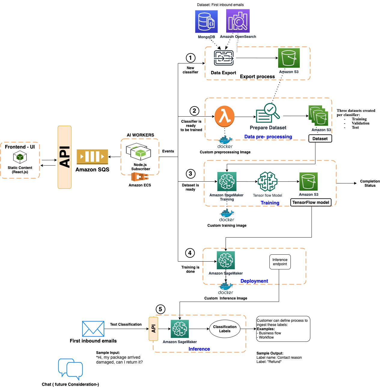
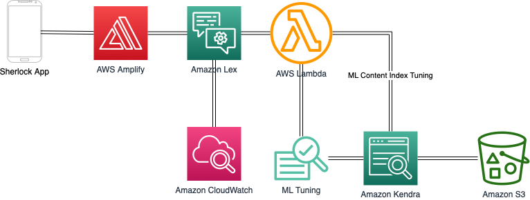
The following diagram is the architecture implemented for the solution:
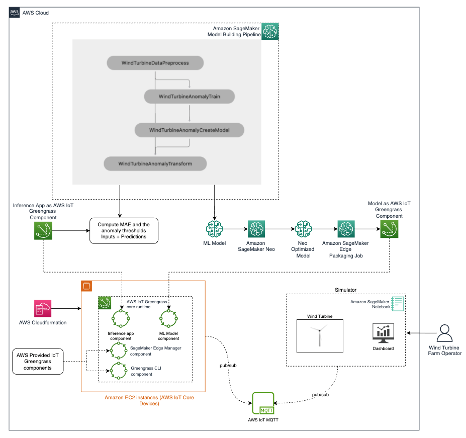
We can broadly divide the architecture into the following phases:
-
Model training
- Prepare the data and train an anomaly detection model using Amazon SageMaker Pipelines. SageMaker Pipelines helps orchestrate your training pipeline with your own custom code. It also outputs the Mean Absolute Error (MAE) and other threshold values used to calculate anomalies.
-
Compile and package the model
- Compile the model using Neo, so that it can be optimized for the target hardware (in this case, an EC2 instance).
- Use the SageMaker Edge packaging job API to package the model as an AWS IoT Greengrass component. The Edge Manager API has a native integration with AWS IoT Greengrass APIs.
-
Build and package the inference application
- Build and package the inference application as an AWS IoT Greengrass component. This application uses the computed threshold, the model, and some custom code to accept the data coming from turbines, perform anomaly detection, and return results.
-
Set up AWS IoT Greengrass on edge devices
- Set up a fleet of AWS IoT Greengrass core devices. In this architecture, we use EC2 instances to act as core devices. We spin up five EC2 instances via AWS CloudFormation and install the AWS IoT Greengrass core runtime on those instances.
-
Deploy to edge devices
- Deploy the following on each edge device:
- An ML model packaged as an AWS IoT Greengrass component.
- An inference application packaged an AWS IoT Greengrass component. This also sets up the connection to AWS IoT Core MQTT.
- The AWS-provided Edge Manager Greengrass component.
- The AWS-provided AWS IoT Greengrass CLI component (only needed for development and debugging purposes).
- Deploy the following on each edge device:
-
Run the end-to-end solution
- Run the simulator, which generates measurements for the wind turbines, which are sent to the edge devices using MQTT.
- Because the notebook and the EC2 instances running AWS IoT Greengrass are on different networks, we use AWS IoT Core to relay MQTT messages between them. In a real scenario, the wind turbine would send the data to the anomaly detection device using a local communication, for example, an AWS IoT Greengrass MQTT broker component.
- The inference app and model running in the anomaly detection device predicts if the received data is anomalous or not, and sends the result to the monitoring application via MQTT through AWS IoT Core.
- The application displays the data and anomaly signal on the simulator dashboard.
To know more on how to deploy this solution architecture, please refer to the GitHub Repository related to this post.
In the following sections, we go deeper into the details of how to implement this solution.
Dataset
The solution uses raw turbine data collected from real wind turbines. The dataset is provided as part of the solution. It has the following features:
- nanoId – ID of the edge device that collected the data
- turbineId – ID of the turbine that produced this data
- arduino_timestamp – Timestamp of the Arduino that was operating this turbine
- nanoFreemem: Amount of free memory in bytes
- eventTime – Timestamp of the row
- rps – Rotation of the rotor in rotations per second
- voltage – Voltage produced by the generator in milivolts
- qw, qx, qy, qz – Quaternion angular acceleration
- gx, gy, gz – Gravity acceleration
- ax, ay, az – Linear acceleration
- gearboxtemp – Internal temperature
- ambtemp – External temperature
- humidity – Air humidity
- pressure – Air pressure
- gas – Air quality
- wind_speed_rps – Wind speed in rotations per second
For more information, refer to Monitor and Manage Anomaly Detection Models on a fleet of Wind Turbines with Amazon SageMaker Edge Manager.
Data preparation and training
The data preparation and training are performed using SageMaker Pipelines. Pipelines is the first purpose-built, easy-to-use continuous integration and continuous delivery (CI/CD) service for ML. With Pipelines, you can create, automate, and manage end-to-end ML workflows at scale. Because it’s purpose-built for ML, Pipelines helps automate different steps of the ML workflow, including data loading, data transformation, training and tuning, and deployment. For more information, refer to Amazon SageMaker Model Building Pipelines.
Model compilation
We use Neo for model compilation. It automatically optimizes ML models for inference on cloud instances and edge devices to run faster with no loss in accuracy. ML models are optimized for a target hardware platform, which can be a SageMaker hosting instance or an edge device based on processor type and capabilities, for example if there is a GPU or not. The compiler uses ML to apply the performance optimizations that extract the best available performance for your model on the cloud instance or edge device. For more information, see Compile and Deploy Models with Neo.
Model packaging
To use a compiled model with Edge Manager, you first need to package it. In this step, SageMaker creates an archive consisting of the compiled model and the Neo DLR runtime required to run it. It also signs the model for integrity verification. When you deploy the model via AWS IoT Greengrass, the create_edge_packaging_job API automatically creates an AWS IoT Greengrass component containing the model package, which is ready to be deployed to the devices.
The following code snippet shows how to invoke this API:
To allow the API to create an AWS IoT Greengrass component, you must provide the following additional parameters under OutputConfig:
- The
PresetDeploymentTypeasGreengrassV2Component -
PresetDeploymentConfigto provide theComponentNameandComponentVersionthat AWS IoT Greengrass uses to publish the component - The
ComponentVersionandModelVersionmust be inmajor.minor.patchformat
The model is then published as an AWS IoT Greengrass component.
Create the inference application as an AWS IoT Greengrass component
Now we create an inference application component that we can deploy to the device. This application component loads the ML model, receives data from wind turbines, performs anomaly detections, and sends the result back to the simulator. This application can be a native application that receives the data locally on the edge devices from the turbines or any other client application over a gRPC interface.
To create a custom AWS IoT Greengrass component, perform the following steps:
- Provide the code for the application as single files or as an archive. The code needs to be uploaded to an S3 bucket in the same Region where we registered the AWS IoT Greengrass devices.
- Create a recipe file, which specifies the component’s configuration parameters, component dependencies, lifecycle, and platform compatibility.
The component lifecycle defines the commands that install, run, and shut down the component. For more information, see AWS IoT Greengrass component recipe reference. We can define the recipe either in JSON or YAML format. Because the inference application requires the model and Edge Manager agent to be available on the device, we need to specify dependencies to the ML model packaged as an AWS IoT Greengrass component and the Edge Manager Greengrass component.
- When the recipe file is ready, create the inference component by invoking the create_component_version API. See the following code:
Inference application
The inference application connects to AWS IoT Core to receive messages from the simulated wind turbine and send the prediction results to the simulator dashboard.
It publishes to the following topics:
-
wind-turbine/{turbine_id}/dashboard/update– Updates the simulator dashboard -
wind-turbine/{turbine_id}/label/update– Updates the model loaded status on simulator -
wind-turbine/{turbine_id}/anomalies– Publishes anomaly results to the simulator dashboard
It subscribes to the following topic:
-
wind-turbine/{turbine_id}/raw-data– Receives raw data from the turbine
Set up AWS IoT Core devices
Next, we need to set up the devices that run the anomaly detection application by installing the AWS IoT Greengrass core software. For this post, we use five EC2 instances that act as the anomaly detection devices. We use AWS CloudFormation to launch the instances. To install the AWS IoT Greengrass core software, we provide a script in the instance UserData as shown in the following code:
Each EC2 instance is associated to a single virtual wind turbine. In a real scenario, multiple wind turbines could also communicate to a single device in order to reduce the solution costs.
To learn more about how to set up AWS IoT Greengrass software on a core device, refer to Install the AWS IoT Greengrass Core software. The complete CloudFormation template is available in the GitHub repository.
Create an AWS IoT Greengrass deployment
When the devices are up and running, we can deploy the application. We create a deployment with a configuration containing the following components:
- ML model
- Inference application
- Edge Manager
- AWS IoT Greengrass CLI (only needed for debugging purposes)
For each component, we must specify the component version. We can also provide additional configuration data, if necessary. We create the deployment by invoking the create_deployment API. See the following code:
The targetArn argument defines where to run the deployment. The thing group ARN is specified to deploy this configuration to all devices belonging to the thing group. The thing group is created already as part of the setup of the solution architecture.
The aws.greengrass.SageMakerEdgeManager component is an AWS-provided component by AWS IoT Greengrass. At the time of writing, the latest version is 1.1.0. You need to configure this component with the SageMaker edge device fleet name and S3 bucket location. You can find these parameters on the Edge Manager console, where the fleet was created during the setup of the solution architecture.
aws.samples.windturbine.detector is the inference application component created earlier.
aws.samples.windturbine.model is the anomaly detection ML model component created earlier.
Run the simulator
Now that everything is in place, we can start the simulator. The simulator is run from a Python notebook and performs two tasks:
- Simulate the physical wind turbine and display a dashboard for each wind turbine.
- Exchange data with the devices via AWS IoT MQTT using the following topics:
-
wind-turbine/{turbine_id}/raw-data– Publishes the raw turbine data. -
wind-turbine/{turbine_id}/label/update– Receives model loaded or not loaded status from the inference application. -
wind-turbine/{turbine_id}/anomalies– Receives anomalies published by inference application. -
wind-turbine/{turbine_id}/dashboard/update– Receives recent buffered data by the turbines.
-
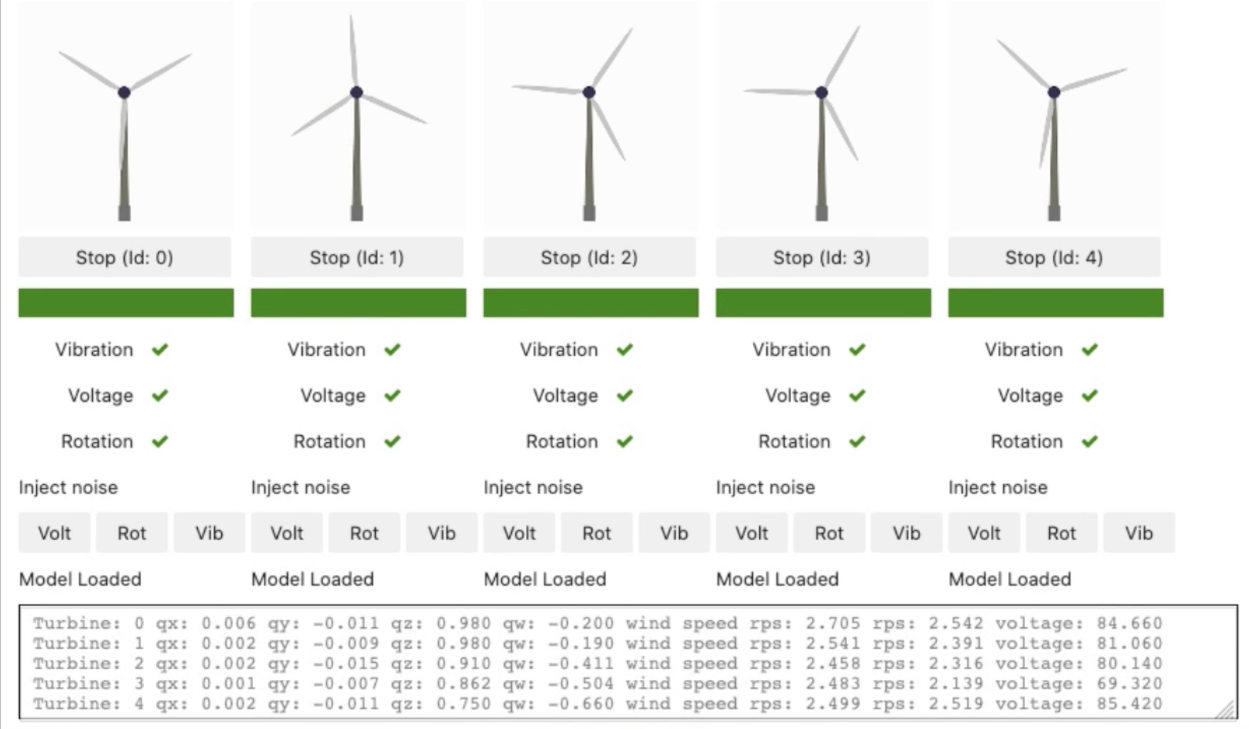
We can use the simulator UI to start and stop the virtual wind turbine and inject noise in the Volt, Rot, and Vib measurements to simulate anomalies that are detected by the application running on the device. In the following screenshot, the simulator shows a virtual representation of five wind turbines that are currently running. We can choose Stop to stop any of the turbines, or choose Volt, Rot, or Vib to inject noise in the turbines. For example, if we choose Volt for turbine with ID 0, the Voltage status changes from a green check mark to a red x, denoting the voltage readings of the turbine are anomalous.
Conclusion
Securely and reliably maintaining the lifecycle of an ML model deployed across a fleet of devices isn’t an easy task. However, with Edge Manager and AWS IoT Greengrass, we can reduce the implementation effort and operational cost of such a solution. This solution increases the agility in experimenting and optimizing the ML model with full automation of the ML pipelines, from data acquisition, data preparation, model training, model validation, and deployment to the devices.
In addition to the benefits described, Edge Manager offers further benefits, like having access to a device fleet dashboard on the Edge Manager console, which can display near-real-time health of the devices by capturing heartbeat requests. You can use this inference data with Amazon SageMaker Model Monitor to check for data and model quality drift issues.
To build a solution for your own needs, get the code and artifacts from the GitHub repo. The repository shows two different ways of deploying the models:
- Using IoT jobs
- Using AWS IoT Greengrass (covered in this post)
Although this post focuses on deployment using AWS IoT Greengrass, interested readers look at the solution using IoT jobs as well to better understand the differences.
About the Authors
 Vikesh Pandey is a Machine Learning Specialist Specialist Solutions Architect at AWS, helping customers in the Nordics and wider EMEA region design and build ML solutions. Outside of work, Vikesh enjoys trying out different cuisines and playing outdoor sports.
 Massimiliano Angelino is Lead Architect for the EMEA Prototyping team. During the last 3 and half years he has been an IoT Specialist Solution Architect with a particular focus on edge computing, and he contributed to the launch of AWS IoT Greengrass v2 service and its integration with Amazon SageMaker Edge Manager. Based in Stockholm, he enjoys skating on frozen lakes.