The Columbia Center of AI Technology announced its inaugural recipients last year.Read More
Josh Miele: Amazon’s resident MacArthur Fellow
Miele has merged a lifelong passion for science with a mission to make the world more accessible for people with disabilities.Read More
Announcing the launch of the model copy feature for Amazon Comprehend custom models
Technology trends and advancements in digital media in the past decade or so have resulted in the proliferation of text-based data. The potential benefits of mining this text to derive insights, both tactical and strategic, is enormous. This is called natural language processing (NLP). You can use NLP, for example, to analyze your product reviews for customer sentiments, train a custom entity recognizer model to identify product types of interest based on customer comments, or train a custom text classification model to determine the most popular product categories.
Amazon Comprehend is an NLP service with ready-made intelligence to extract insights about the content of documents. It develops insights by recognizing the entities, key phrases, language, sentiments, and other common elements in a document. Amazon Comprehend Custom uses automatic machine learning (Auto ML) to build NLP models on your behalf using your own data. This enables you to detect entities unique to your business or classify text or documents as per your requirements. Additionally, you can automate your entire NLP workflow with easy-to-use APIs.
Today we’re happy to announce the launch of the Amazon Comprehend custom model copy feature, which allows you to automatically copy your Amazon Comprehend custom models from a source account to designated target accounts in the same Region without requiring access to the datasets that the model was trained and evaluated on. Starting today, you can use the AWS Management Console, AWS Command Line Interface (AWS CLI), or the boto3 APIs (Python SDK for AWS) to copy trained custom models from a source account to a designated target account. This new feature is available for both Amazon Comprehend custom classification and custom entity recognition models.
Benefits of the model copy feature
This new feature has the following benefits:
- Multi-account MLOps strategy – Train a model one time and ensure predictable deployment in multiple environments in different accounts.
- Faster deployment – You can quickly copy a trained model between accounts, avoiding the time taken to retrain in every account.
- Protect sensitive datasets – Now you no longer need to share the datasets between different accounts or users. The training data needs to be available only on the account where the training is done. This is very important for certain industries like financial services, where data isolation and sandboxing are essential to meet regulatory requirements.
- Easy collaboration – Partners or vendors can now easily train in Amazon Comprehend Custom and share the models with their customers.
How model copy works
With the new model copy feature, you can copy custom models between AWS accounts in the same Region in a two-stage process. First, a user in one AWS account (account A), shares a custom model that’s in their account. Then, a user in another AWS account (account B) imports the model into their account.
Share a model
To share a custom model in account A, the user attaches an AWS Identity and Access Management (IAM) resource-based policy to a model version. This policy authorizes an entity in account B, such as an IAM user or role, to import the model version into Amazon Comprehend in their AWS account. You can configure a resource-based policy either through the console or with the Amazon Comprehend custom PutResourcePolicy API.
Import a model
To import the model to account B, the user of this account provides Amazon Comprehend with the necessary details, such as the Amazon Resource Name (ARN) of the model. When they import the model, this user creates a new custom model in their AWS account that replicates the model that they imported. This model is fully trained and ready for inference jobs, such as document classification or named entity recognition. If the model is encrypted with an AWS Key Management Service (AWS KMS) key in the source, then the service role specified while importing the model needs to have access to the KMS key in order to decrypt the model during import. The target account can also specify a KMS key to encrypt the model during import. The importing of the shared model is also available both on the console and as an API.
Solution overview
To demonstrate the functionality of the model copy feature, we show you how to train, share, and import an Amazon Comprehend custom entity recognition model using both the Amazon Comprehend console and the AWS CLI. For this demonstration, we use two different accounts. The steps are applicable to Amazon Comprehend custom classification as well. The required steps are as follows:
- Train an Amazon Comprehend custom entity recognition model in the source account.
- Define the IAM resource policy for the trained model to allow cross-account access.
- Copy the trained model from the source account to the target account.
- Test the copied model through a batch job.
Train an Amazon Comprehend custom entity recognition model in the source account
The first step is to train an Amazon Comprehend custom entity recognition model in the source account. As an input dataset for the training, we use a CSV entity list and training documents for recognizing AWS service offerings in a given document. Make sure that the entity list and training documents are in an Amazon Simple Storage Service (Amazon S3) bucket in the source account. For instructions, see Adding Documents to Amazon S3.
Create an IAM role for Amazon Comprehend and provide required access to the S3 bucket with the training data. Note the role ARN and S3 bucket paths to use in later steps.
Train a model with the AWS CLI
Create an entity recognizer using the following AWS CLI command. Substitute your parameters for the S3 paths, IAM role, and Region. The response returns back the EntityRecognizerArn.
The status of the training job can be monitored by calling the describe-entity-recognizer and checking the Status in the response.
Train a model via the console
To train a model via the console, complete the following steps:
- On the Amazon Comprehend console, under Customization, create a new custom entity recognizer model.
- Provide a model name and version.
- For Language, choose Engligh.
- For Custom entity type, add
AWS_OFFERING.
To train a custom entity recognition model, you can choose one of two ways to provide data to Amazon Comprehend: annotations or entity lists. For simplicity, use the entity list method.
- For Data format, select CSV file.
- For Training type, select Using entity list and training docs.
- Provide the S3 location paths for the entity list CSV and training data.
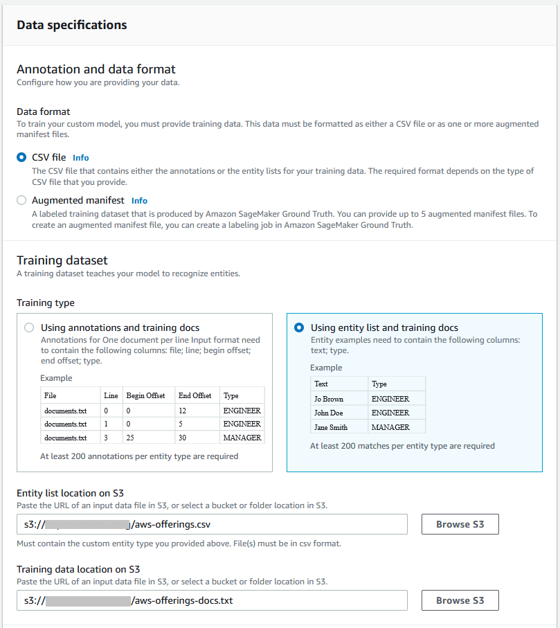
- To grant permissions to Amazon Comprehend to access your S3 bucket, create an IAM service-linked role.
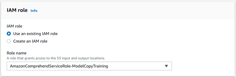
In the Resource-based policy section, you can authorize access for the model version. The accounts you grant access to can import this model into their account. We skip this step for now and add the policy after the model is trained and we’re satisfied with the model performance.
- Choose Create.
This submits your custom entity recognizer, which goes through a number of models, tunes your hyperparameters, and checks for cross-validation to make sure that your model is robust. These are all the same activities that data scientists perform.
Define the IAM resource policy for the trained model to allow cross-account access
When we’re satisfied with the training performance, we can go ahead and share the specific model version by adding a resource policy.
Add a resource-based policy from the AWS CLI
Authorize importing the model from the target account by adding a resource policy on the model, as shown in the following code. The policy can be tightly scoped to a particular model version and target principal. Substitute your trained entity recognizer ARN and target account to provide access to.
Add a resource-based policy via the console
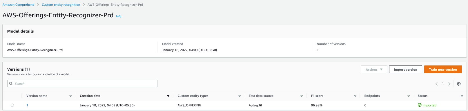
When the training is complete, a custom entity recognition model version is generated. We can choose the trained model and version to view the training details, including performance of the trained model.

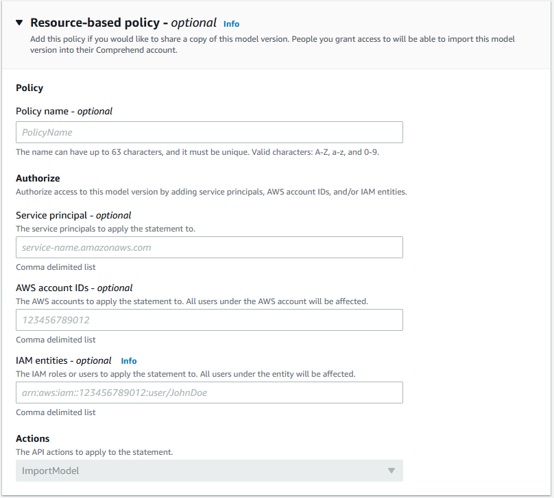
To update the policy, complete the following steps:
- On the Tags, VPC & Policy tab, edit the resource-based policy.
- Provide the policy name, Amazon Comprehend service principal (
comprehend.amazonaws.com), target account ID, and IAM users in the target account authorized to import the model version.
We specify root as the IAM entity to authorize all users in the target account.
- Make a note of the model resource ARN, which we use later during the import process.

Copy the trained model from the source account to the target account
Now the model is trained and shared from the source account. The authorized target account user can import the model and create a copy of the model in their own account.
To import a model, you need to specify the source model ARN and service role for Amazon Comprehend to perform the copy action on your account. You can specify an optional AWS KMS ID to encrypt the model in your target account.
Import the model through AWS CLI
To import your model with the AWS CLI, enter the following code:
Import the model via the console
To import the model via the console, complete the following steps:
- On the Amazon Comprehend console, under Custom entity recognition, choose Import version.
- For Model version ARN, enter the ARN for the model trained in the source account.
- Enter a model name and version for the target.

- Provide a service account role and choose Confirm to start the model import process.
After the model status changes to Imported, we can view the model details, including the performance details of the trained model.
Test the copied model through a batch job
We test the copied model in the target account by detecting custom entities with a batch job. To test the model, download the test file and place it in an S3 bucket in your target account. Create an IAM role for Amazon Comprehend and provide the required access to the S3 bucket with the test data. You use the role ARN and S3 bucket paths that you noted earlier.
When the job is complete, you can verify the inference data in the specified output S3 bucket.
Test the model with the AWS CLI
To test the model using the AWS CLI, enter the following code:
Test the model via the console
To test the model via the console, complete the following steps:
- On the Amazon Comprehend console, choose Analysis jobs and choose Create job.
- For Name, enter a name for the job.
- For Analysis type¸ choose Custom entity recognition.
- Choose the model name and version of the imported model.

- Provide the S3 paths for the test file for the job and the output location where Amazon Comprehend stores the result.

- Choose or create an IAM role with permission to access the S3 buckets.

- Choose Create job.
When your analysis job is complete, you have JSON files in your output S3 bucket path, which you can download to verify the results of the entity recognition from the imported model.

Conclusion
In this post, we demonstrated the Amazon Comprehend custom entity model copy feature. This feature gives you the ability to train an Amazon Comprehend custom entity recognition or classification model in one account and then share the model with another account in the same Region. This simplifies the multi-account strategy where the model can be trained one time and shared between accounts within same Region without having to retrain or share the training datasets. This allows for a predicable deployment in every account as part of your MLOps workflow. For more information, see our documentation on Comprehend custom copy, or try out the walkthrough in this post either via the console or using a cloud shell with the AWS CLI.
As of this writing, the model copy feature in Amazon Comprehend is available in the following Regions:
- US East (Ohio)
- US East (N. Virginia)
- US West (Oregon)
- Asia Pacific (Mumbai)
- Asia Pacific (Seoul)
- Asia Pacific (Singapore)
- Asia Pacific (Sydney)
- Asia Pacific (Tokyo)
- EU (Frankfurt)
- EU (Ireland)
- EU (London)
- AWS GovCloud (US-West)
Give the feature a try, and please send us feedback either via the AWS forum for Amazon Comprehend or through your usual AWS support contacts.
About the Authors
 Premkumar Rangarajan is an AI/ML specialist solutions architect at Amazon Web Services and has previously authored the book Natural Language Processing with AWS AI services. He has 26 years of experience in the IT industry in a variety of roles, including delivery lead, integration specialist, and enterprise architect. He helps enterprises of all sizes adopt AI and ML to solve for their real-world challenges.
 Chethan Krishna is a Senior Partner Solutions Architect in India. He works with Strategic AWS Partners for establishing a robust cloud competency, adopting AWS best practices and solving customer challenges. He is a builder and enjoys experimenting with AI/ML, IoT, and analytics.
 Sriharsha M S is an AI/ML specialist solution architect in the Strategic Specialist team at Amazon Web Services. He works with strategic AWS customers who are taking advantage of AI/ML to solve complex business problems. He provides technical guidance and design advice to implement AI/ML applications at scale. His expertise spans application architecture, bigdata, analytics and machine learning.
Balance your data for machine learning with Amazon SageMaker Data Wrangler
Amazon SageMaker Data Wrangler is a new capability of Amazon SageMaker that makes it faster for data scientists and engineers to prepare data for machine learning (ML) applications by using a visual interface. It contains over 300 built-in data transformations so you can quickly normalize, transform, and combine features without having to write any code.
Today, we’re excited to announce new transformations that allow you to balance your datasets easily and effectively for ML model training. We demonstrate how these transformations work in this post.
New balancing operators
The newly announced balancing operators are grouped under the Balance data transform type in the ADD TRANFORM pane.

Currently, the transform operators support only binary classification problems. In binary classification problems, the classifier is tasked with classifying each sample to one of two classes. When the number of samples in the majority class (bigger) is considerably larger than the number of samples in the minority (smaller) class, the dataset is considered imbalanced. This skew is challenging for ML algorithms and classifiers because the training process tends to be biased towards the majority class.
Balancing schemes, which augment the data to be more balanced before training the classifier, were proposed to address this challenge. The simplest balancing methods are either oversampling the minority class by duplicating minority samples or undersampling the majority class by removing majority samples. The idea of adding synthetic minority samples to tabular data was first proposed in the Synthetic Minority Oversampling Technique (SMOTE), where synthetic minority samples are created by interpolating pairs of the original minority points. SMOTE and other balancing schemes were extensively studied empirically and shown to improve prediction performance in various scenarios, as per the publication To SMOTE, or not to SMOTE.
Data Wrangler now supports the following balancing operators as part of the Balance data transform:
- Random oversampler – Randomly duplicate minority samples
- Random undersampler – Randomly remove majority samples
- SMOTE – Generate synthetic minority samples by interpolating real minority samples

Let’s now discuss the different balancing operators in detail.
Random oversample
Random oversampling includes selecting random examples from the minority class with a replacement and supplementing the training data with multiple copies of this instance. Therefore, it’s possible that a single instance may be selected multiple times. With the Random oversample transform type, Data Wrangler automatically oversamples the minority class for you by duplicating the minority samples in your dataset.
Random undersample
Random undersampling is the opposite of random oversampling. This method seeks to randomly select and remove samples from the majority class, consequently reducing the number of examples in the majority class in the transformed data. The Random undersample transform type lets Data Wrangler automatically undersample the majority class for you by removing majority samples in your dataset.
SMOTE
In SMOTE, synthetic minority samples are added to the data to achieve the desired ratio between majority and minority samples. The synthetic samples are generated by interpolation of pairs of the original minority points. The SMOTE transform supports balancing datasets including numeric and non-numeric features. Numeric features are interpolated by weighted average. However, you can’t apply weighted average interpolation to non-numeric features—it’s impossible to average “dog” and “cat” for example. Instead, non-numeric features are copied from either original minority sample according to the averaging weight.
For example, consider two samples, A and B:
Assume the samples are interpolated with weights 0.3 for sample A and 0.7 for sample B. Therefore, the numeric fields are averaged with these weights to yield 0.3 and 0.6, respectively. The next field is filled with “dog” with probability 0.3 and “cow” with probability 0.7. Similarly, the next one equals “carnivore” with probability 0.3 and “herbivore” with probability 0.7. The random copying is done independently for each feature, so sample C below is a possible result:
This example demonstrates how the interpolation process could result in unrealistic synthetic samples, such as an herbivore dog. This is more common with categorical features but can occur in numeric features as well. Even though some synthetic samples may be unrealistic, SMOTE could still improve classification performance.
To heuristically generate more realistic samples, SMOTE interpolates only pairs that are close in features space. Technically, each sample is interpolated only with its k-nearest neighbors, where a common value for k is 5. In our implementation of SMOTE, only the numeric features are used to calculate the distances between points (the distances are used to determine the neighborhood of each sample). It’s common to normalize the numeric features before calculating distances. Note that the numeric features are normalized only for the purpose of calculating the distance; the resulting interpolated features aren’t normalized.
Let’s now balance the Adult Dataset (also known as the Census Income dataset) using the built-in SMOTE transform provided by Data Wrangler. This multivariate dataset includes six numeric features and eight string features. The goal of the dataset is a binary classification task to predict whether the income of an individual exceeds $50,000 per year or not based on census data.
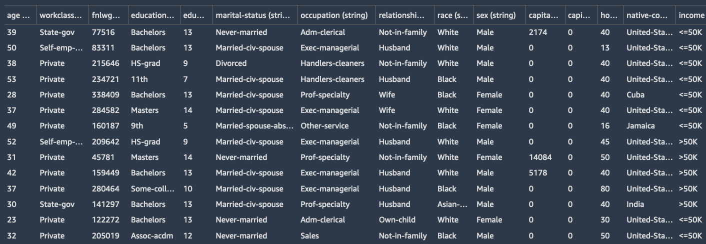
You can also see the distribution of the classes visually by creating a histogram using the histogram analysis type in Data Wrangler. The target distribution is imbalanced and the ratio of records with >50K to <=50K is about 1:4.

We can balance this data using the SMOTE operator found under the Balance Data transform in Data Wrangler with the following steps:
- Choose
incomeas the target column.
We want the distribution of this column to be more balanced.
- Set the desired ratio to
0.66.
Therefore, the ratio between the number of minority and majority samples is 2:3 (instead of the raw ratio of 1:4).
- Choose SMOTE as the transform to use.
- Leave the default values for Number of neighbors to average and whether or not to normalize.

- Choose Preview to get a preview of the applied transformation and choose Add to add the transform to your data flow.
Now we can create a new histogram similar to what we did before to see the realigned distribution of the classes. The following figure shows the histogram of the income column after balancing the dataset. The distribution of samples is now 3:2, as was intended.

We can now export this new balanced data and train a classifier on it, which could yield superior prediction quality.
Conclusion
In this post, we demonstrated how to balance imbalanced binary classification data using Data Wrangler. Data Wrangler offers three balancing operators: random undersampling, random oversampling, and SMOTE to rebalance data in your unbalanced datasets. All three methods offered by Data Wrangler support multi-modal data including numeric and non-numeric features.
As next steps, we recommend you replicate the example in this post in your Data Wrangler data flow to see what we discussed in action. If you’re new to Data Wrangler or SageMaker Studio, refer to Get Started with Data Wrangler. If you have any questions related to this post, please add it in the comment section.
About the Authors
 Yotam Elor is a Senior Applied Scientist at Amazon SageMaker. His research interests are in machine learning, particularly for tabular data.
 Arunprasath Shankar is an Artificial Intelligence and Machine Learning (AI/ML) Specialist Solutions Architect with AWS, helping global customers scale their AI solutions effectively and efficiently in the cloud. In his spare time, Arun enjoys watching sci-fi movies and listening to classical music.
Launch processing jobs with a few clicks using Amazon SageMaker Data Wrangler
Amazon SageMaker Data Wrangler makes it faster for data scientists and engineers to prepare data for machine learning (ML) applications by using a visual interface. Previously, when you created a Data Wrangler data flow, you could choose different export options to easily integrate that data flow into your data processing pipeline. Data Wrangler offers export options to Amazon Simple Storage Service (Amazon S3), SageMaker Pipelines, and SageMaker Feature Store, or as Python code. The export options create a Jupyter notebook and require you to run the code to start a processing job facilitated by SageMaker Processing.
We’re excited to announce the general release of destination nodes and the Create Job feature in Data Wrangler. This feature gives you the ability to export all the transformations that you made to a dataset to a destination node with just a few clicks. This allows you to create data processing jobs and export to Amazon S3 purely via the visual interface without having to generate, run, or manage Jupyter notebooks, thereby enhancing the low-code experience. To demonstrate this new feature, we use the Titanic dataset and show how to export your transformations to a destination node.
Prerequisites
Before we learn how to use destination nodes with Data Wrangler, you should already understand how to access and get started with Data Wrangler. You also need to know what a data flow means with context to Data Wrangler and how to create one by importing your data from the different data sources Data Wrangler supports.
Solution overview
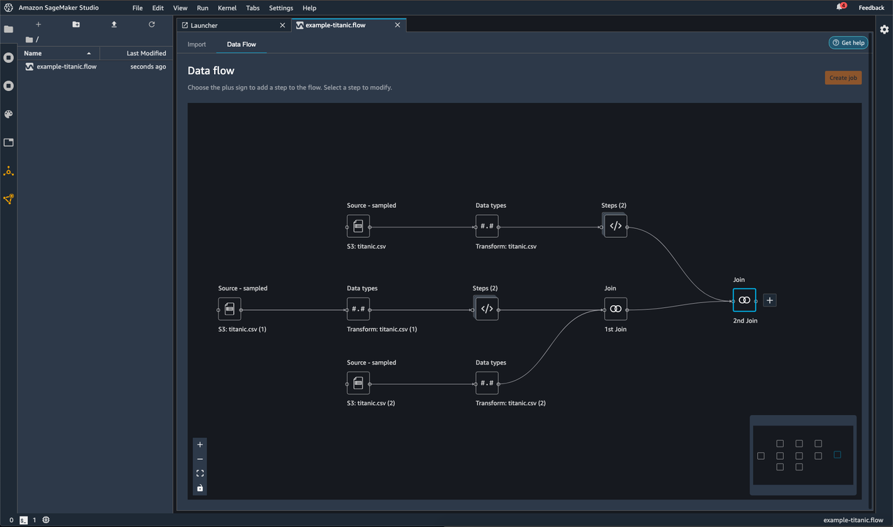
Consider the following data flow named example-titanic.flow:
- It imports the Titanic dataset three times. You can see these different imports as separate branches in the data flow.
- For each branch, it applies a set of transformations and visualizations.
- It joins the branches into a single node with all the transformations and visualizations.
With this flow, you might want to process and save parts of your data to a specific branch or location.
In the following steps, we demonstrate how to create destination nodes, export them to Amazon S3, and create and launch a processing job.
Create a destination node
You can use the following procedure to create destination nodes and export them to an S3 bucket:
- Determine what parts of the flow file (transformations) you want to save.
- Choose the plus sign next to the nodes that represent the transformations that you want to export. (If it’s a collapsed node, you must select the options icon (three dots) for the node).

- Hover over Add destination.

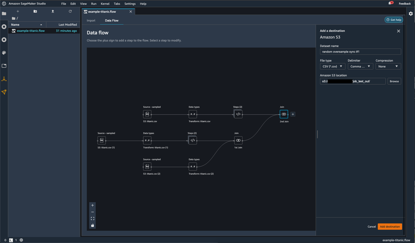
- Choose Amazon S3.

- Specify the fields as shown in the following screenshot.
- For the second join node, follow the same steps to add Amazon S3 as a destination and specify the fields.
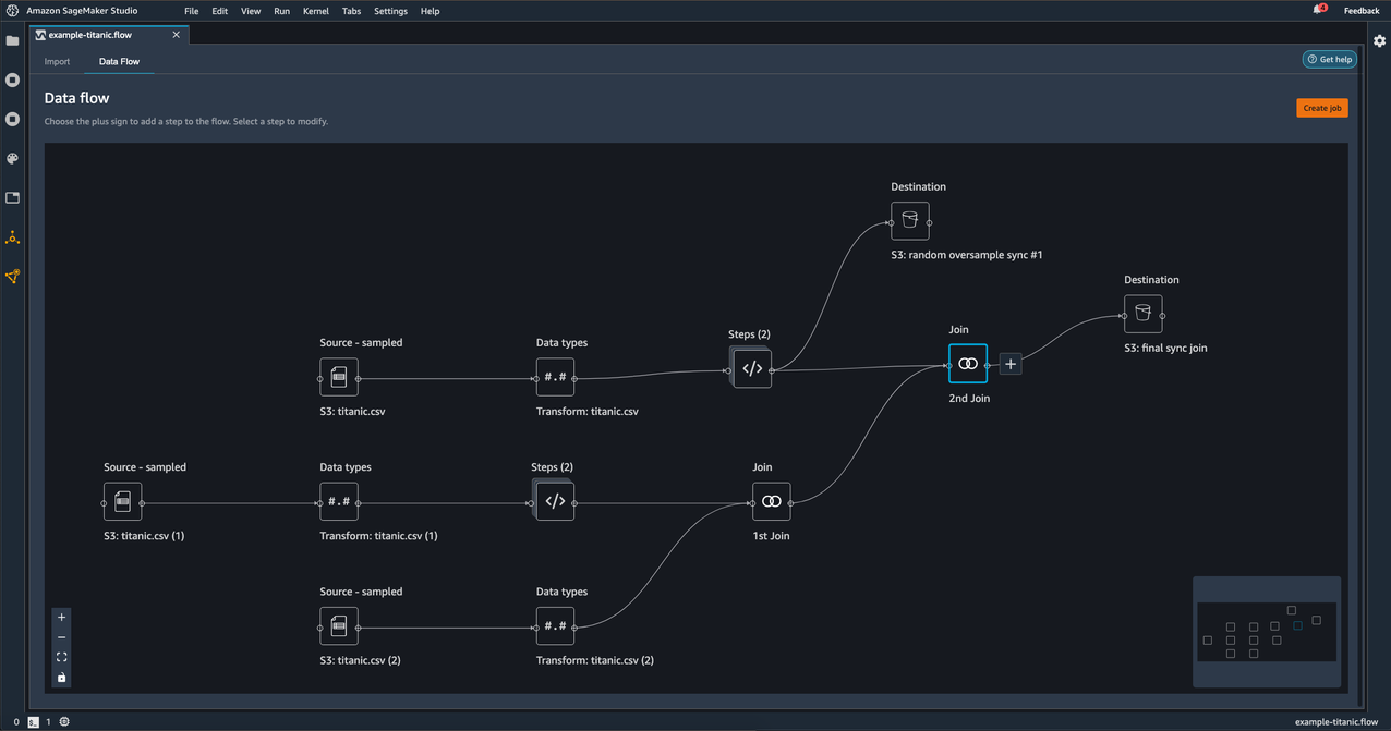
You can repeat these steps as many times as you need for as many nodes you want in your data flow. Later on, you pick which destination nodes to include in your processing job.
Launch a processing job
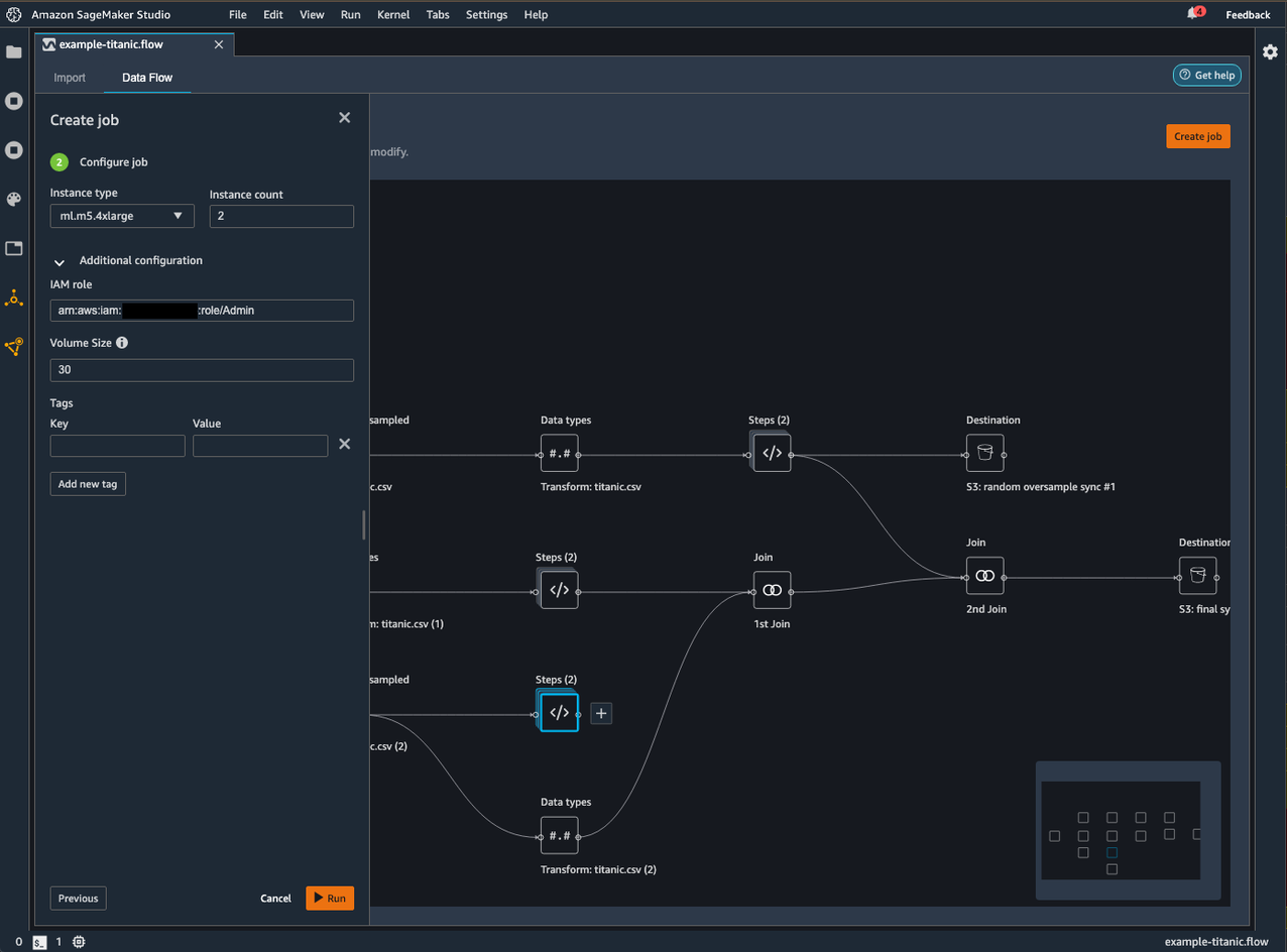
Use the following procedure to create a processing job and choose the destination node where you want to export to:
- On the Data Flow tab, choose Create job.
- For Job name¸ enter the name of the export job.
- Select the destination nodes you want to export.
- Optionally, specify the AWS Key Management Service (AWS KMS) key ARN.
The KMS key is a cryptographic key that you can use to protect your data. For more information about KMS keys, see the AWS Key Developer Guide.
- Choose Next, 2. Configure job.

- Optionally, you can configure the job as per your needs by changing the instance type or count, or adding any tags to associate with the job.
- Choose Run to run the job.
A success message appears when the job is successfully created.

View the final data
Finally, you can use the following steps to view the exported data:
- After you create the job, choose the provided link.
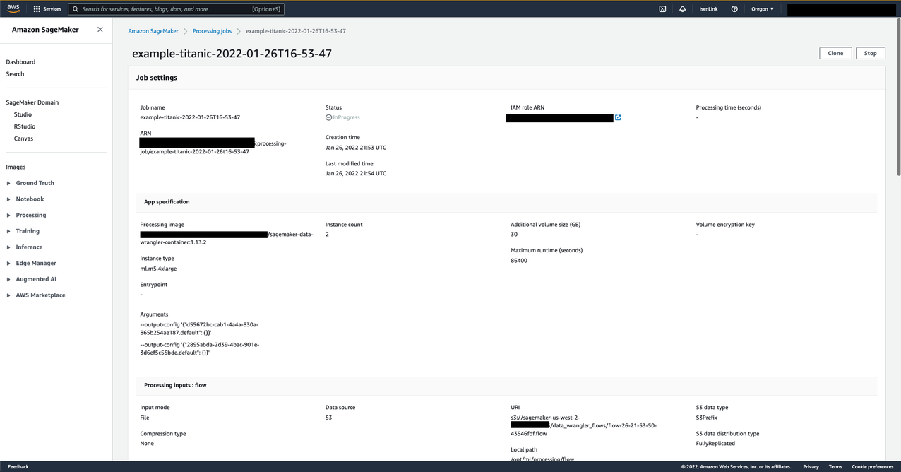
A new tab opens showing the processing job on the SageMaker console.
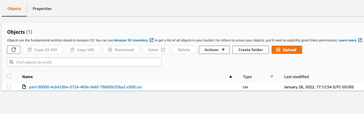
- When the job is complete, review the exported data on the Amazon S3 console.
You should see a new folder with the job name you chose.

- Choose the job name to view a CSV file (or multiple files) with the final data.
FAQ
In this section, we address a few frequently asked questions about this new feature:
- What happened to the Export tab? With this new feature, we removed the Export tab from Data Wrangler. You can still facilitate the export functionality via the Data Wrangler generated Jupyter notebooks from any nodes you created in the data flow with the following steps:
-
- Choose the plus sign next to the node that you want to export.
- Choose Export to.
- Choose Amazon S3 (via Jupyter Notebook).
- Run the Jupyter notebook.

- How many destinations nodes can I include in a job? There is a maximum of 10 destinations per processing job.
- How many destination nodes can I have in a flow file? You can have as many destination nodes as you want.
- Can I add transformations after my destination nodes? No, the idea is destination nodes are terminal nodes that have no further steps afterwards.
- What are the supported sources I can use with destination nodes? As of this writing, we only support Amazon S3 as a destination source. Support for more destination source types will be added in the future. Please reach out if there is a specific one you would like to see.
Summary
In this post, we demonstrated how to use the newly launched destination nodes to create processing jobs and save your transformed datasets directly to Amazon S3 via the Data Wrangler visual interface. With this additional feature, we have enhanced the tool-driven low-code experience of Data Wrangler.
As next steps, we recommend you try the example demonstrated in this post. If you have any questions or want to learn more, see Export or leave a question in the comment section.
About the Authors
 Alfonso Austin-Rivera is a Front End Engineer at Amazon SageMaker Data Wrangler. He is passionate about building intuitive user experiences that spark joy. In his spare time, you can find him fighting gravity at a rock-climbing gym or outside flying his drone.
 Parsa Shahbodaghi is a Technical Writer in AWS specializing in machine learning and artificial intelligence. He writes the technical documentation for Amazon SageMaker Data Wrangler and Amazon SageMaker Feature Store. In his free time, he enjoys meditating, listening to audiobooks, weightlifting, and watching stand-up comedy. He will never be a stand-up comedian, but at least his mom thinks he’s funny.
 Balaji Tummala is a Software Development Engineer at Amazon SageMaker. He helps support Amazon SageMaker Data Wrangler and is passionate about building performant and scalable software. Outside of work, he enjoys reading fiction and playing volleyball.
Arunprasath Shankar is an Artificial Intelligence and Machine Learning (AI/ML) Specialist Solutions Architect with AWS, helping global customers scale their AI solutions effectively and efficiently in the cloud. In his spare time, Arun enjoys watching sci-fi movies and listening to classical music.
Prepare and analyze JSON and ORC data with Amazon SageMaker Data Wrangler
Amazon SageMaker Data Wrangler is a new capability of Amazon SageMaker that makes it faster for data scientists and engineers to prepare data for machine learning (ML) applications via a visual interface. Data preparation is a crucial step of the ML lifecycle, and Data Wrangler provides an end-to-end solution to import, prepare, transform, featurize, and analyze data for ML in a seamless, visual, low-code experience. It lets you easily and quickly connect to AWS components like Amazon Simple Storage Service (Amazon S3), Amazon Athena, Amazon Redshift, and AWS Lake Formation, and external sources like Snowflake. Data Wrangler also supports standard data types such as CSV and Parquet.
Data Wrangler now additionally supports Optimized Row Columnar (ORC), JavaScript Object Notation (JSON), and JSON Lines (JSONL) file formats:
- ORC – The ORC file format provides a highly efficient way to store Hive data. It was designed to overcome limitations of the other Hive file formats. Using ORC files improves performance when Hive is reading, writing, and processing data. ORC is widely used in the Hadoop ecosystem.
- JSON – The JSON file format is a lightweight, commonly used data interchange format.
- JSONL – JSON Lines, also called newline-delimited JSON, is a convenient format for storing structured data that may be processed one record at a time.
You can preview ORC, JSON, and JSONL data prior to importing the datasets into Data Wrangler. After you import the data, you can also use one of the newly launched transformers to work with columns that contain JSON strings or arrays that are commonly found in nested JSONs.
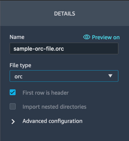
Import and analyze ORC data with Data Wrangler
Importing ORC data is in Data Wrangler is easy and similar to importing files in any other supported formats. Browse to your ORC file in Amazon S3 and in the DETAILS pane, choose ORC as the file type during import.
If you’re new to Data Wrangler, review Get Started with Data Wrangler. Also, see Import to learn about the various import options.
Import and analyze JSON data with Data Wrangler
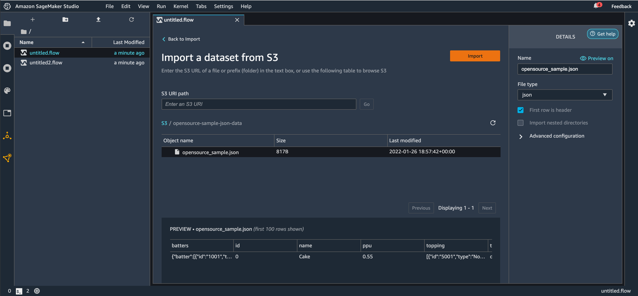
Now let’s import files in JSON format with Data Wrangler and work with columns that contain JSON strings or arrays. We also demonstrate how to deal with nested JSONs. With Data Wrangler, importing JSON files from Amazon S3 is a seamless process. This is similar to importing files in any other supported formats. After you import the files, you can preview the JSON files as shown in the following screenshot. Make sure to set the file type to JSON in the DETAILS pane.
Next, let’s work on structured columns in the imported JSON file.
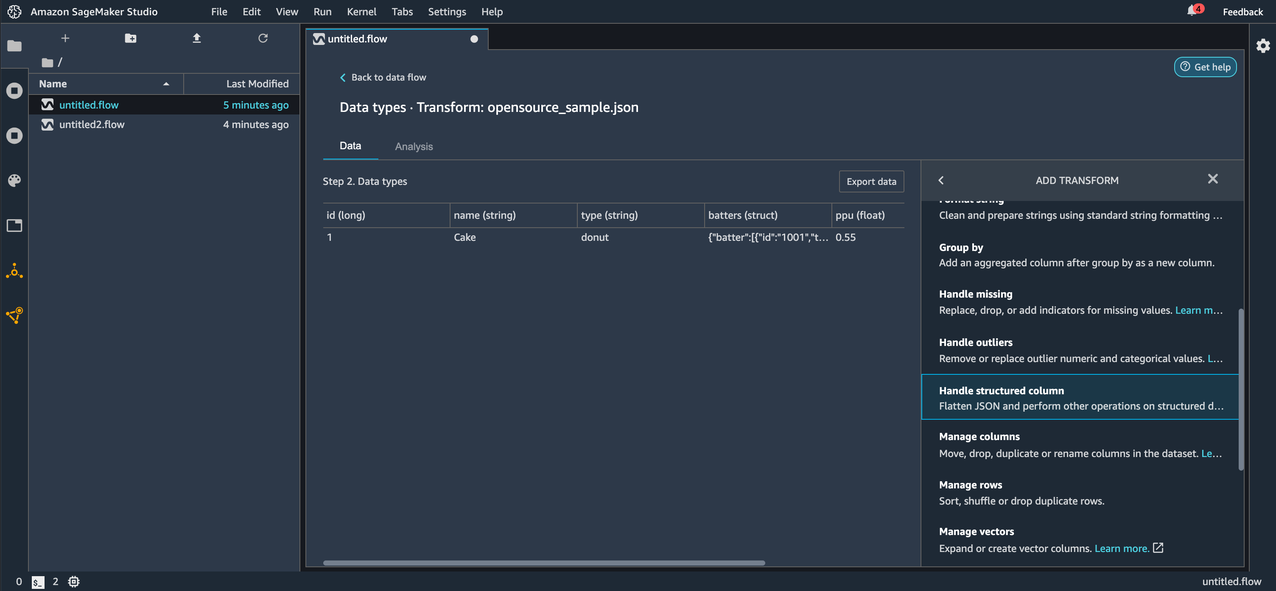
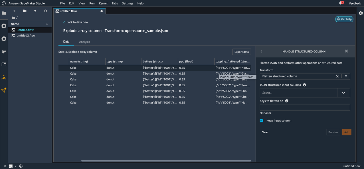
To deal with structured columns in JSON files, Data Wrangler is introducing two new transforms: Flatten structured column and Explode array column, which can be found under the Handle structured column option in the ADD TRANSFORM pane.
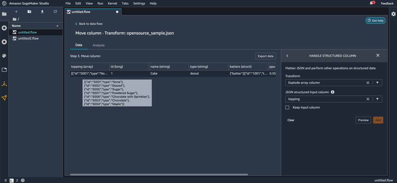
Let’s start by applying the Explode array column transform to one of the columns in our imported data. Before applying the transform, we can see the column topping is an array of JSON objects with id and type keys.
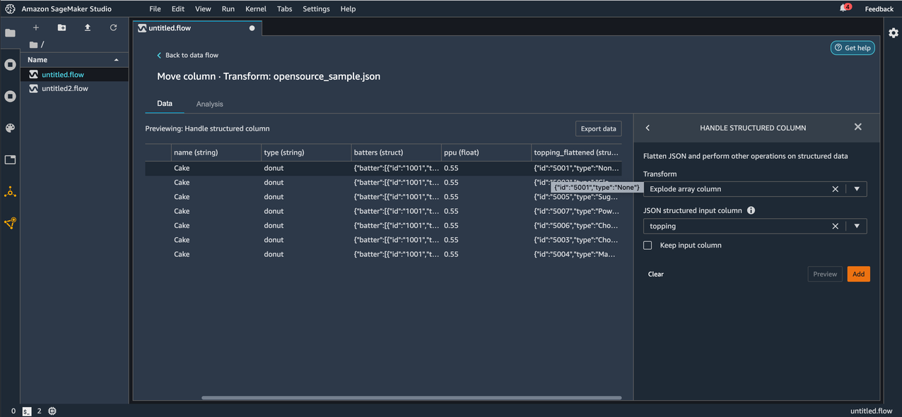
After we apply the transform, we can observe the new rows added as a result. Each element in the array is now a new row in the resulting DataFrame.
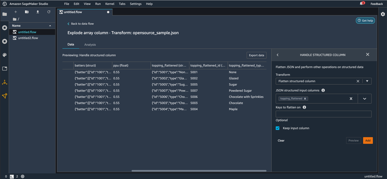
Now let’s apply the Flatten structured column transform on the topping_flattened column that was created as a result of the Explode array column transformation we applied in the previous step.
Before applying the transform, we can see the keys id and type in the topping_flattened column.
After applying the transform, we can now observe the keys id and type under the topping_flattened column as new columns topping_flattened_id and topping_flattened_type, which are created as a result of the transformation. You also have the option to flatten only specific keys by entering the comma separated key names for Keys to flatten on. If left empty, all the keys inside the JSON string or struct are flattened.
Conclusion
In this post, we demonstrated how to import file formats in ORC and JSON easily with Data Wrangler. We also applied the newly launched transformations that allow us to transform any structured columns in JSON data. This makes working with columns that contain JSON strings or arrays a seamless experience.
As next steps, we recommend you replicate the demonstrated examples in your own Data Wrangler visual interface. If you have any questions related to Data Wrangler, feel free to leave them in the comment section.
About the Authors
Balaji Tummala is a Software Development Engineer at Amazon SageMaker. He helps support Amazon SageMaker Data Wrangler and is passionate about building performant and scalable software. Outside of work, he enjoys reading fiction and playing volleyball.
Arunprasath Shankar is an Artificial Intelligence and Machine Learning (AI/ML) Specialist Solutions Architect with AWS, helping global customers scale their AI solutions effectively and efficiently in the cloud. In his spare time, Arun enjoys watching sci-fi movies and listening to classical music.
Alexa AI co-organizes special sessions at Interspeech
Sessions on multidevice scenarios, inclusive and fair speech technologies, trustworthy speech processing, and speech intelligibility prediction seek paper submissions.Read More
René Vidal wins Edward J. McCluskey Technical Achievement Award
The Amazon Scholar and Johns Hopkins University professor was honored for “pioneering contributions to subspace clustering”.Read More
The engineering behind Alexa’s contextual speech recognition
How Alexa scales machine learning models to millions of customers.Read More
Run AutoML experiments with large parquet datasets using Amazon SageMaker Autopilot.
Starting today, you can use Amazon SageMaker Autopilot to tackle regression and classification tasks on large datasets up to 100 GB. Additionally, you can now provide your datasets in either CSV or Apache Parquet content types.
Businesses are generating more data than ever. A corresponding demand is growing for generating insights from these large datasets to shape business decisions. However, successfully training state-of-the-art machine learning (ML) algorithms on these large datasets can be challenging. Autopilot automates this process and provides a seamless experience for running automated machine learning (AutoML) on large datasets up to 100 GB.
Autopilot subsamples your large datasets automatically to fit the maximum supported limit while preserving the rare class in case of class imbalance. Class imbalance is an important problem to be aware of in ML, especially when dealing with large datasets. Consider a fraud detection dataset where only a small fraction of transactions is expected to be fraudulent. In this case, Autopilot subsamples only the majority class, non-fraudulent transactions, while preserving the rare class, fraudulent transactions.
When you run an AutoML job using Autopilot, all relevant information for subsampling is stored in Amazon CloudWatch. Navigate to the log group for /aws/sagemaker/ProcessingJobs, search for the name of your AutoML job, and choose the CloudWatch log stream that includes -db- in its name.
Many of our customers prefer the Parquet content type to store their large datasets. This is generally due to its compressed nature, support for advanced data structures, efficiency, and low-cost operations. This data can often reach up to tens or even hundreds of GBs. Now, you can directly bring these Parquet datasets to Autopilot. You can either use our API or navigate to Amazon SageMaker Studio to create an Autopilot job with a few clicks. You can specify the input location of your Parquet dataset as a single file or multiple files specified as a manifest file. Autopilot automatically detects the content type of your dataset, parses it, extracts meaningful features, and trains multiple ML algorithms.
You can get started using our sample notebook for running AutoML using Autopilot on Parquet datasets.
About the Authors
 H. Furkan Bozkurt, Machine Learning Engineer, Amazon SageMaker Autopilot.
 Valerio Perrone, Applied Science Manager, Amazon SageMaker Autopilot.