EBSCOlearning offers corporate learning and educational and career development products and services for businesses, educational institutions, and workforce development organizations. As a division of EBSCO Information Services, EBSCOlearning is committed to enhancing professional development and educational skills.
In this post, we illustrate how EBSCOlearning partnered with AWS Generative AI Innovation Center (GenAIIC) to use the power of generative AI in revolutionizing their learning assessment process. We explore the challenges faced in traditional question-answer (QA) generation and the innovative AI-driven solution developed to address them.
In the rapidly evolving landscape of education and professional development, the ability to effectively assess learners’ understanding of content is crucial. EBSCOlearning, a leader in the realm of online learning, recognized this need and embarked on an ambitious journey to transform their assessment creation process using cutting-edge generative AI technology.
Amazon Bedrock is a fully managed service that offers a choice of high-performing foundation models (FMs) from leading AI companies such as AI21 Labs, Anthropic, Cohere, Meta, Mistral AI, Stability AI, and Amazon through a single API, along with a broad set of capabilities to build generative AI applications with security, privacy, and responsible AI, and is well positioned to address these types of tasks.
The challenge: Scaling quality assessments
EBSCOlearning’s learning paths—comprising videos, book summaries, and articles—form the backbone of a multitude of educational and professional development programs. However, the company faced a significant hurdle: creating high-quality, multiple-choice questions for these learning paths was a time-consuming and resource-intensive process.
Traditionally, subject matter experts (SMEs) would meticulously craft each question set to be relevant, accurate, and to align with learning objectives. Although this approach guaranteed quality, it was slow, expensive, and difficult to scale. As EBSCOlearning’s content library continues to grow, so does the need for a more efficient solution.
Enter AI: A promising solution
Recognizing the potential of AI to address this challenge, EBSCOlearning partnered with the GenAIIC to develop an AI-powered question generation system. The goal was ambitious: to create an automated solution that could produce high-quality, multiple-choice questions at scale, while adhering to strict guidelines on bias, safety, relevance, style, tone, meaningfulness, clarity, and diversity, equity, and inclusion (DEI). The QA pairs had to be grounded in the learning content and test different levels of understanding, such as recall, comprehension, and application of knowledge. Additionally, explanations were needed to justify why an answer was correct or incorrect.
The team faced several key challenges:
- Making sure AI-generated questions matched the quality of human-created ones
- Developing a system that could handle diverse content types
- Implementing robust quality control measures
- Creating a scalable solution that could grow with EBSCOlearning’s needs
Crafting the AI solution
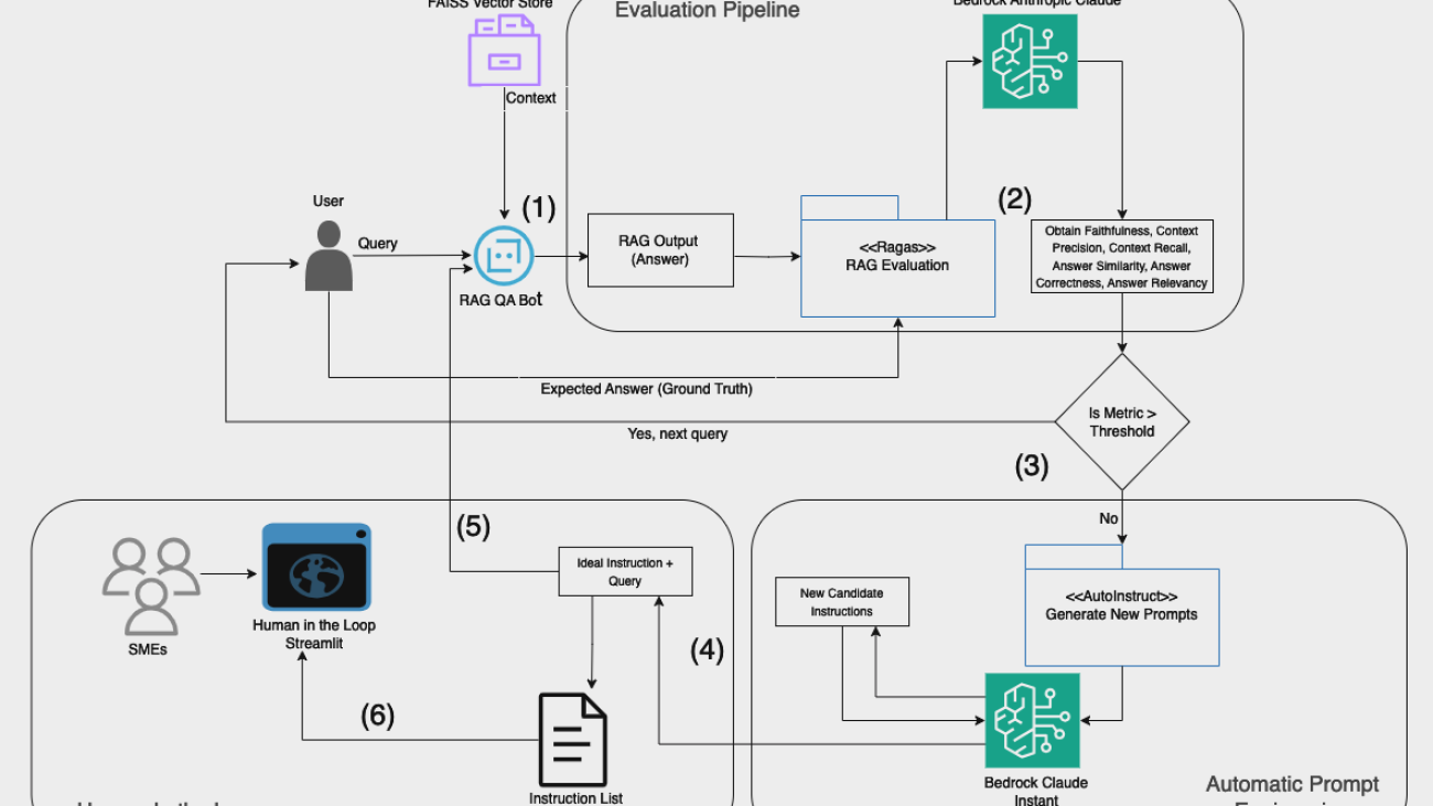
The GenAIIC team developed a sophisticated pipeline using the power of large language models (LLMs), specifically Anthropic’s Claude 3.5 Sonnet in Amazon Bedrock. This pipeline is illustrated in the following figure and consists of several key components: QA generation, multifaceted evaluation, and intelligent revision.

QA generation
The process begins with the QA generation component. This module takes in the learning content—which could be a video transcript, book summary, or article—and generates an initial set of multiple-choice questions using in-context learning.
EBSCOlearning experts and GenAIIC scientists worked together to develop a sophisticated prompt engineering approach using Anthropic’s Claude 3.5 Sonnet model in Amazon Bedrock. To align with EBSCOlearning’s high standards, the prompt includes:
- Detailed guidelines on what constitutes a high-quality question, covering aspects such as relevance, clarity, difficulty level, and objectivity
- Instructions to match the conversational style of the original content
- Directives to include diversity and inclusivity in the language and scenarios used
- Few-shot examples to enable in-context learning for the AI model
The system aims to generate up to seven questions for each piece of content, each with four answer choices including a correct answer, and detailed explanations for why each answer is correct or incorrect.
Multifaceted evaluation
After the initial set of questions is generated, it undergoes a rigorous evaluation process. This multifaceted approach makes sure that the questions adhere to all quality standards and guidelines. The evaluation process includes three phases: LLM-based guideline evaluation, rule-based checks, and a final evaluation.
LLM-based guideline evaluation
In collaboration with EBSCOlearning, the GenAIIC team manually developed a comprehensive set of evaluation guidelines covering fundamental requirements for multiple-choice questions, such as validity, accuracy, and relevance. Additionally, they incorporated EBSCOlearning’s specific standards for diversity, equity, inclusion, and belonging (DEIB), in addition to style and tone preferences. The AI system evaluates each question according to the established guidelines and generates a structured output that includes detailed reasoning along with a rating on a three-point scale, where 1 indicates invalid, 2 indicates partially valid, and 3 indicates valid. This rating is later used for revising the questions.
This process presented several significant challenges. The primary challenge was making sure that the AI model could effectively assess multiple complex guidelines simultaneously without overlooking any crucial aspects. This was particularly difficult because the evaluation needed to consider so many different factors—all while maintaining consistency across questions.
To overcome the challenge of LLMs potentially overlooking guidelines when presented with them all at one time, the evaluation process was split into smaller manageable tasks by getting the AI model to focus on fewer guidelines at a time or evaluating smaller chunks of questions in parallel. This way, each guideline receives focused attention, resulting in a more accurate and comprehensive evaluation. Additionally, the system was designed with modularity in mind, streamlining the addition or removal of guidelines. Because of this flexibility, the evaluation process can adapt quickly to new requirements or changes in educational standards.
By generating detailed, structured feedback for each question, including numerical ratings, concise summaries, and in-depth reasoning, the system provides invaluable insights for continual improvement. This level of detail allows for a nuanced understanding of how well each question aligns with the established criteria, offering possibilities for targeted enhancements to the question generation process.
Rule-based checks
Some quantitative aspects of question quality proved challenging for the AI to consistently evaluate. For instance, the team noticed that correct answers were often longer than incorrect ones, making them straightforward to identify. To address this, they developed a custom algorithm that analyzes answer lengths and flags potential issues without relying on the LLM’s judgment.
Final evaluation
Beyond evaluating individual questions, the system also assesses the entire set of questions for a given piece of content. This step checks for duplicates, promotes diversity in the types of questions asked, and verifies that the set as a whole provides a comprehensive assessment of the learning material.
Intelligent revision
One key component of the pipeline is the intelligent revision module. This is where the iterative improvement happens. When the evaluation process flags issues with a question—whether it’s a guideline violation or a structural problem—the question is sent back for revision. The AI model is provided with specific feedback on how it can address the specific violation and directs it to fix the issue by revising or replacing the QA.
The power of iteration
The whole pipeline goes through multiple iterations until the question aligns with all of the specified quality standards. If after several attempts a question still doesn’t meet the criteria, it’s flagged for human review. This iterative approach makes sure that the final output isn’t merely a raw AI generation, but a refined product that has gone through multiple checks and improvements.
Throughout the development process, the team maintained a strong focus on iterative tracking of changes. They implemented a unique history tracking system so they could monitor the evolution of each question through multiple rounds of generation, evaluation, and revision. This approach not only provided valuable insights into the AI model’s decision-making process, but also allowed for targeted improvements to the system over time. By closely tracking the AI model’s performance across multiple iterations, we were able to fine-tune our prompts and evaluation criteria, resulting in a significant improvement in output quality.
Scalability and robustness
With EBSCOlearning’s vast content library in mind, the team built scalability into the core of their solution. They implemented multithreading capabilities, allowing the system to process multiple pieces of content simultaneously. They also developed sophisticated retry mechanisms to handle potential API failures or invalid outputs so the system remained reliable even when processing large volumes of content.
The results: A game-changer for learning assessment
By combining these components—intelligent generation, comprehensive evaluation, and adaptive revision—EBSCOlearning and the GenAIIC team created a system that not only automates the process of creating assessment questions but does so with a level of quality that rivals human-created content. This pipeline represents a significant leap forward in the application of AI to educational content creation, promising to revolutionize how learning assessments are developed and delivered.
The impact of this AI-powered solution on EBSCOlearning’s assessment creation process has been nothing short of transformative. Feedback from EBSCOlearning’s subject matter experts has been overwhelmingly positive, with the AI-generated questions meeting or exceeding the quality of manually created ones in many cases.
Key benefits of the new system include:
- Dramatically reduced time and cost for assessment creation
- Consistent quality across a wide range of subjects and content types
- Improved scalability, allowing EBSCOlearning to keep pace with their growing content library
- Enhanced learning experiences for end users, with more diverse and engaging assessments
“The Generative AI Innovation Center’s automated solution for generating multiple-choice questions and answers considerably accelerated the timeline for deployment of assessments for our online learning platform. Their approach of leveraging advanced language models and implementing carefully constructed guidelines in collaboration with our subject matter experts and product management team has resulted in assessment material that is accurate, relevant, and of high quality. This solution is saving us considerable time and effort, and will enable us to scale assessments across the wide range of skills development resources on our platform.”
—Michael Laddin, Senior Vice President & General Manager, EBSCOlearning.
Here are two examples of generated QA.
Question 1: What does the Consumer Relevancy model proposed by Crawford and Mathews assert about human values in business transactions?
- A. Human values are less important than monetary value.
- B. Human values and monetary value are equally important in all transactions.
- C. Human values are more important than traditional value propositions.
- D. Human values are irrelevant compared to monetary value in business transactions.
Correct answer: C
Answer explanations:
- A. This is contrary to what the Consumer Relevancy model asserts. The model emphasizes the importance of human values over traditional value propositions.
- B. While this might seem balanced, it doesn’t reflect the emphasis placed on human values in the Consumer Relevancy model. The model asserts that human values are more important.
- C. This correctly reflects the assertion of the Consumer Relevancy model as described in the Book Summary. The model emphasizes the importance of human values over traditional value propositions.
- D. This is the opposite of what the Consumer Relevancy model asserts. The model emphasizes the importance of human values, not their irrelevance.
Overall: The Book Summary states that the Consumer Relevancy model asserts that human values are more important than traditional value propositions and that businesses must recognize this need for human values as the contemporary currency of commerce.
Question 2: According to Sara N. King, David G. Altman, and Robert J. Lee, what is the primary benefit of leaders having clarity about their own values?
- A. It guarantees success in all leadership positions.
- B. It helps leaders make more fulfilling career choices.
- C. It eliminates all conflicts in the workplace environment.
- D. It ensures leaders always make ethically perfect decisions.
Correct answer: B
Answer explanations:
- A. The Book Summary does not suggest that clarity about values guarantees success in all leadership positions. This is an overstatement of the benefits.
- B. This is the correct answer, as the Book Summary states that clarity about values allows leaders to make more fulfilling career choices and recognize conflicts with their core values.
- C. While understanding one’s values can help in managing conflicts, the Book Summary does not claim it eliminates all workplace conflicts. This is an exaggeration of the benefits.
- D. The Book Summary does not state that clarity about values ensures leaders always make ethically perfect decisions. This is an unrealistic expectation not mentioned in the content.
Overall: The Book Summary emphasizes that having clarity about one’s own values allows leaders to make more fulfilling career choices and helps them recognize when they are participating in actions that conflict with their core values.
Looking to the future
For EBSCOlearning, this project is the first step towards their goal of scaling assessments across their entire online learning platform. They’re already planning to expand the system’s capabilities, including:
- Adapting the solution to handle more complex, technical content
- Incorporating additional question types beyond multiple-choice
- Exploring ways to personalize assessments based on individual learner profiles
The potential applications of this technology extend far beyond EBSCOlearning’s current use case. From personalized learning paths to adaptive testing, the possibilities for AI in education and professional development are vast and exciting.
Conclusion: A new era of learning assessment
The collaboration between EBSCOlearning and the GenAIIC demonstrates the transformative power of AI when applied thoughtfully to real-world challenges. By combining cutting-edge technology with deep domain expertise, they’ve created a solution that not only solves a pressing business need but also has the potential to enhance learning experiences for millions of people. This solution is slated to produce assessment questions for hundreds and eventually thousands of learning paths in EBSCOlearning’s curriculum.
As we look to the future of education and professional development, it’s clear that AI will play an increasingly important role. The success of this project serves as a compelling example of how AI can be used to create more efficient, effective, and engaging learning experiences.
For businesses and educational institutions alike, the message is clear: embracing AI isn’t just about keeping up with technology trends—it’s about unlocking new possibilities to better serve learners and drive innovation in education. As EBSCOlearning’s journey shows, the future of learning assessment is here, and it’s powered by AI. Consider how such a solution can enrich your own e-learning content and delight your customers with high quality and on-point assessments. To get started, contact your AWS account manager. If you don’t have an AWS account manager, contact sales. Visit Generative AI Innovation Center to learn more about our program.
About the authors
 Yasin Khatami is a Senior Applied Scientist at the Generative AI Innovation Center. With more than a decade of experience in artificial intelligence (AI), he implements state-of-the-art AI products for AWS customers to drive innovation, efficiency and value for customer platforms. His expertise is in generative AI, large language models (LLM), multi-agent techniques, and multimodal learning.
 Yifu Hu is an Applied Scientist at the Generative AI Innovation Center. He develops machine learning and generative AI solutions for diverse customer challenges across various industries. Yifu specializes in creative problem-solving, with expertise in AI/ML technologies, particularly in applications of large language models and AI agents.
 Aude Genevay is a Senior Applied Scientist at the Generative AI Innovation Center, where she helps customers tackle critical business challenges and create value using generative AI. She holds a PhD in theoretical machine learning and enjoys turning cutting-edge research into real-world solutions.
 Mike Laddin is Senior Vice President & General Manager of EBSCOlearning, a division of EBSCO Information Services. EBSCOlearning offers highly acclaimed online products and services for companies, educational institutions, and workforce development organizations. Mike oversees a team of professionals focused on unlocking the potential of people and organizations with on-demand upskilling and microlearning solutions. He has over 25 years of experience as both an entrepreneur and software executive in the information services industry. Mike received an MBA from the Lally School of Management at Rensselaer Polytechnic Institute, and outside of work he is an avid boater.
 Alyssa Gigliotti is a Content Strategy and Product Operations Manager at EBSCOlearning, where she collaborates with her team to design top-tier microlearning solutions focused on enhancing business and power skills. With a background in English, professional writing, and technical communications from UMass Amherst, Alyssa combines her expertise in language with a strategic approach to educational content. Alyssa’s in-depth knowledge of the product and voice of the customer allows her to actively engage in product development planning to ensure her team continuously meets the needs of users. Outside the professional sphere, she is both a talented artist and a passionate reader, continuously seeking inspiration from creative and literary pursuits.
Read More


 Jiten Dedhia is a Sr. AIML Solutions Architect with over 20 years of experience in the software industry. He has helped Fortune 500 companies with their AIML/Generative AI needs.
 Sapna Maheshwari is a Sr. Solutions Architect at AWS, with a passion for designing impactful tech solutions. She is an engaging speaker who enjoys sharing her insights at conferences.


 Joe Travaglini is a Principal Product Manager on the AWS Field Experiences (AFX) team who focuses on helping the AWS salesforce deliver value to AWS customers through generative AI. Prior to AFX, Joe led the product management function for Amazon Elastic File System, Amazon ElastiCache, and Amazon MemoryDB.
 Jonathan Garcia is a Sr. Software Development Manager based in Seattle with over a decade of experience at AWS. He has worked on a variety of products, including data visualization tools and mobile applications. He is passionate about serverless technologies, mobile development, leveraging Generative AI, and architecting innovative high-impact solutions. Outside of work, he enjoys golfing, biking, and exploring the outdoors.
 Umesh Mohan is a Software Engineering Manager at AWS, where he has been leading a team of talented engineers for over three years. With more than 15 years of experience in building data warehousing products and software applications, he is now focusing on the use of generative AI to drive smarter and more impactful solutions. Outside of work, he enjoys spending time with his family and playing tennis.


 Suren Gunturu is a Data Scientist working in the Generative AI Innovation Center, where he works with various AWS customers to solve high-value business problems. He specializes in building ML pipelines using large language models, primarily through Amazon Bedrock and other AWS Cloud services.
 Varun Kumar is a Staff Data Scientist at Tealium, leading its research program to provide high-quality data and AI solutions to its customers. He has extensive experience in training and deploying deep learning and machine learning models at scale. Additionally, he is accelerating Tealium’s adoption of foundation models in its workflow including RAG, agents, fine-tuning, and continued pre-training.
 Vidya Sagar Ravipati is a Science Manager at the Generative AI Innovation Center, where he leverages his vast experience in large-scale distributed systems and his passion for machine learning to help AWS customers across different industry verticals accelerate their AI and cloud adoption.
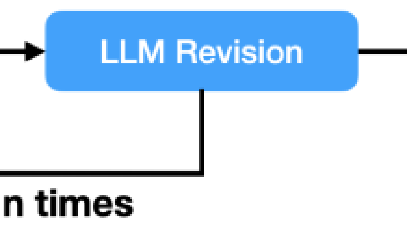


 Preston Tuggle is a Sr. Specialist Solutions Architect working on generative AI.
 Niithiyn Vijeaswaran is a GenAI Specialist Solutions Architect at AWS. His area of focus is generative AI and AWS AI Accelerators. He holds a Bachelor’s degree in Computer Science and Bioinformatics. Niithiyn works closely with the Generative AI GTM team to enable AWS customers on multiple fronts and accelerate their adoption of generative AI. He’s an avid fan of the Dallas Mavericks and enjoys collecting sneakers.
 Shane Rai is a Principal GenAI Specialist with the AWS World Wide Specialist Organization (WWSO). He works with customers across industries to solve their most pressing and innovative business needs using the breadth of cloud-based AI/ML AWS services, including model offerings from top tier foundation model providers.

 Archana Inapudi is a Senior Solutions Architect at AWS, supporting a strategic customer. She has over a decade of cross-industry expertise leading strategic technical initiatives. Archana is an aspiring member of the AI/ML technical field community at AWS. Prior to joining AWS, Archana led a migration from traditional siloed data sources to Hadoop at a healthcare company. She is passionate about using technology to accelerate growth, provide value to customers, and achieve business outcomes.
 Manju Prasad is a Senior Solutions Architect at Amazon Web Services. She focuses on providing technical guidance in a variety of technical domains, including AI/ML. Prior to joining AWS, she designed and built solutions for companies in the financial services sector and also for a startup. She has worked in all layers of the software stack, ranging from webdev to databases, and has experience in all levels of the software development lifecycle. She is passionate about sharing knowledge and fostering interest in emerging talent.
 Amit Arora is an AI and ML Specialist Architect at Amazon Web Services, helping enterprise customers use cloud-based machine learning services to rapidly scale their innovations. He is also an adjunct lecturer in the MS data science and analytics program at Georgetown University in Washington, D.C.
 Antara Raisa is an AI and ML Solutions Architect at Amazon Web Services supporting strategic customers based out of Dallas, Texas. She also has previous experience working with large enterprise partners at AWS, where she worked as a Partner Success Solutions Architect for digital-centered customers.


 Abhishek Maligehalli Shivalingaiah is a Senior Generative AI Solutions Architect at AWS, specializing in Amazon Q Business. With a deep passion for using agentic AI frameworks to solve complex business challenges, he brings nearly a decade of expertise in developing data and AI solutions that deliver tangible value for enterprises. Beyond his professional endeavors, Abhishek is an artist who finds joy in creating portraits of family and friends, expressing his creativity through various artistic mediums.
 Marcel Pividal is a Senior AI Services Solutions Architect in the World-Wide Specialist Organization, bringing over 22 years of expertise in transforming complex business challenges into innovative technological solutions. As a thought leader in generative AI implementation, he specializes in developing secure, compliant AI architectures for enterprise-scale deployments across multiple industries.
 Sachi Sharma is a Senior Software Engineer at Amazon Q Business, specializing in generative and agentic AI. Beyond her professional pursuits, Sachi is an avid reader and coffee lover, and enjoys driving, particularly long, scenic drives.
 Manjukumar Patil is a Software Engineer at Amazon Q Business with a passion for designing and scaling AI-driven distributed systems. In his free time, he loves hiking and exploring national parks.
 James Gung is a Senior Applied Scientist at AWS whose research spans diverse topics related to conversational AI and agentive systems. Outside of work, he enjoys spending time with his family, traveling, playing violin, and bouldering.
 Najih is a Senior Software Engineer at AWS Q Business. He is passionate about designing and scaling AI based distributed systems, and excels at bringing innovative solutions to complex challenges. Outside of work, he enjoys lifting and martial arts, particularly MMA.