Organizations face the challenge to manage data, multiple artificial intelligence and machine learning (AI/ML) tools, and workflows across different environments, impacting productivity and governance. A unified development environment consolidates data processing, model development, and AI application deployment into a single system. This integration streamlines workflows, enhances collaboration, and accelerates AI solution development from concept to production.
The next generation of Amazon SageMaker is the center for your data, analytics, and AI. SageMaker brings together AWS AI/ML and analytics capabilities and delivers an integrated experience for analytics and AI with unified access to data. Amazon SageMaker Unified Studio is a single data and AI development environment where you can find and access your data and act on it using AWS analytics and AI/ML services, for SQL analytics, data processing, model development, and generative AI application development.
With SageMaker Unified Studio, you can efficiently build generative AI applications in a trusted and secure environment using Amazon Bedrock. You can choose from a selection of high-performing foundation models (FMs) and advanced customization and tooling such as Amazon Bedrock Knowledge Bases, Amazon Bedrock Guardrails, Amazon Bedrock Agents, and Amazon Bedrock Flows. You can rapidly tailor and deploy generative AI applications, and share with the built-in catalog for discovery.
In this post, we demonstrate how you can use SageMaker Unified Studio to create complex AI workflows using Amazon Bedrock Flows.
Solution overview
Consider FinAssist Corp, a leading financial institution developing a generative AI-powered agent support application. The solution offers the following key features:
- Complaint reference system – An AI-powered system providing quick access to historical complaint data, enabling customer service representatives to efficiently handle customer follow-ups, support internal audits, and aid in training new staff.
- Intelligent knowledge base – A comprehensive data source of resolved complaints that quickly retrieves relevant complaint details, resolution actions, and outcome summaries.
- Streamlined workflow management – Enhanced consistency in customer communications through standardized access to past case information, supporting compliance checks and process improvement initiatives.
- Flexible query capability – A straightforward interface supporting various query scenarios, from customer inquiries about past resolutions to internal reviews of complaint handling procedures.
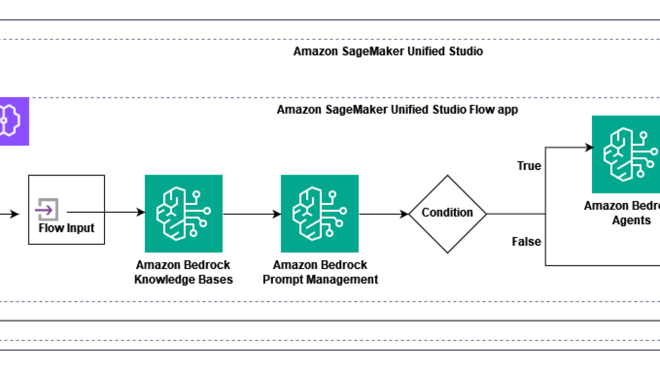
Let’s explore how SageMaker Unified Studio and Amazon Bedrock Flows, integrated with Amazon Bedrock Knowledge Bases and Amazon Bedrock Agents, address these challenges by creating an AI-powered complaint reference system. The following diagram illustrates the solution architecture.

The solution uses the following key components:
- SageMaker Unified Studio – Provides the development environment
- Flow app – Orchestrates the workflow, including:
- Knowledge base queries
- Prompt-based classification
- Conditional routing
- Agent-based response generation
The workflow processes user queries through the following steps:
- A user submits a complaint-related question.
- The knowledge base provides relevant complaint information.
- The prompt classifies if the query is about resolution timing.
- Based on the classification using the condition, the application takes the following action:
- Routes the query to an AI agent for specific resolution responses.
- Returns general complaint information.
- The application generates an appropriate response for the user.
Prerequisites
For this example, you need the following:
- Access to SageMaker Unified Studio. (You will need the SageMaker Unified Studio portal URL from your administrator). You can authenticate using either:
- AWS Identity and Access Management (IAM) user credentials.
- Single sign-on (SSO) credentials with AWS IAM Identity Center.
- The IAM user or IAM Identity Center user must have appropriate permissions for:
- SageMaker Unified Studio.
- Amazon Bedrock (including Amazon Bedrock Flows, Amazon Bedrock Agents, Amazon Bedrock Prompt Management, and Amazon Bedrock Knowledge Bases).
- For more information, refer to Identity-based policy examples.
- Access to Amazon Bedrock FMs (make sure these are enabled for your account), for example:Anthropic’s Claude 3 Haiku (for the agent).
- Configure access to your Amazon Bedrock serverless models for Amazon Bedrock in SageMaker Unified Studio projects.
- Amazon Titan Embedding (for the knowledge base).
- Sample complaint data prepared in CSV format for creating the knowledge base.
Prepare your data
We have created a sample dataset to use for Amazon Bedrock Knowledge Bases. This dataset has information of complaints received by customer service representatives and resolution information.The following is an example from the sample dataset:
Create a project
In SageMaker Unified Studio, users can use projects to collaborate on various business use cases. Within projects, you can manage data assets in the SageMaker Unified Studio catalog, perform data analysis, organize workflows, develop ML models, build generative AI applications, and more.
To create a project, complete the following steps:
- Open the SageMaker Unified Studio landing page using the URL from your admin.
- Choose Create project.
- Enter a project name and optional description.
- For Project profile, choose Generative AI application development.
- Choose Continue.

- Complete your project configuration, then choose Create project.
Create a prompt
Let’s create a reusable prompt to capture the instructions for FMs, which we will use later while creating the flow application. For more information, see Reuse and share Amazon Bedrock prompts.
- In SageMaker Unified Studio, on the Build menu, choose Prompt under Machine Learning & Generative AI.

- Provide a name for the prompt.
- Choose the appropriate FM (for this example, we choose Claude 3 Haiku).
- For Prompt message, we enter the following:
- Choose Save.

- Choose Create version.
Create a chat agent
Let’s create a chat agent to handle specific resolution responses. Complete the following steps:
- In SageMaker Unified Studio, on the Build menu, choose Chat agent under Machine Learning & Generative AI.
- Provide a name for the prompt.
- Choose the appropriate FM (for this example, we choose Claude 3 Haiku).
- For Enter a system prompt, we enter the following:
- Choose Save.

- After the agent is saved, choose Deploy.
- For Alias name, enter
demoAlias. - Choose Deploy.
Create a flow
Now that we have our prompt and agent ready, let’s create a flow that will orchestrate the complaint handling process:
- In SageMaker Unified Studio, on the Build menu, choose Flow under Machine Learning & Generative AI.

- Create a new flow called demo-flow.

Add a knowledge base to your flow application
Complete the following steps to add a knowledge base node to the flow:
- In the navigation pane, on the Nodes tab, choose Knowledge Base.
- On the Configure tab, provide the following information:
- For Node name, enter a name (for example,
complaints_kb). - Choose Create new Knowledge Base.
- For Node name, enter a name (for example,
- In the Create Knowledge Base pane, enter the following information:
- For Name, enter a name (for example,
complaints). - For Description, enter a description (for example,
user complaints information). - For Add data sources, select Local file and upload the complaints.txt file.
- For Embeddings model, choose Titan Text Embeddings V2.
- For Vector store, choose OpenSearch Serverless.
- Choose Create.
- For Name, enter a name (for example,

- After you create the knowledge base, choose it in the flow.
- In the details name, provide the following information:
- For Response generation model, choose Claude 3 Haiku.
- Connect the output of the flow input node with the input of the knowledge base node.
- Connect the output of the knowledge base node with the input of the flow output node.

- Choose Save.
Add a prompt to your flow application
Now let’s add the prompt you created earlier to the flow:
- On the Nodes tab in the Flow app builder pane, add a prompt node.
- On the Configure tab for the prompt node, provide the following information:
- For Node name, enter a name (for example,
demo_prompt). - For Prompt, choose
financeAssistantPrompt. - For Version, choose 1.
- Connect the output of the knowledge base node with the input of the prompt node.

- Choose Save.
Add a condition to your flow application
The condition node determines how the flow handles different types of queries. It evaluates whether a query is about resolution timing or general complaint information, enabling the flow to route the query appropriately. When a query is about resolution timing, it will be directed to the chat agent for specialized handling; otherwise, it will receive a direct response from the knowledge base. Complete the following steps to add a condition:
- On the Nodes tab in the Flow app builder pane, add a condition node.
- On the Configure tab for the condition node, provide the following information:
- For Node name, enter a name (for example,
demo_condition). - Under Conditions, for Condition, enter
conditionInput == "T". - Connect the output of the prompt node with the input of the condition node.

- For Node name, enter a name (for example,
- Choose Save.
Add a chat agent to your flow application
Now let’s add the chat agent you created earlier to the flow:
- On the Nodes tab in the Flow app builder pane, add the agent node.
- On the Configure tab for the agent node, provide the following information:
- For Node name, enter a name (for example,
demo_agent). - For Chat agent, choose
DemoAgent. - For Alias, choose
demoAlias.
- For Node name, enter a name (for example,
- Create the following node connections:
- Connect the input of the condition node (
demo_condition) to the output of the prompt node (demo_prompt). - Connect the output of the condition node:
- Set If condition is true to the agent node (
demo_agent). - Set If condition is false to the existing flow output node (
FlowOutputNode).
- Set If condition is true to the agent node (
- Connect the output of the knowledge base node (
complaints_kb) to the input of the following:- The agent node (
demo_agent). - The flow output node (
FlowOutputNode).
- The agent node (
- Connect the output of the agent node (
demo_agent) to a new flow output node namedFlowOutputNode_2.
- Connect the input of the condition node (
- Choose Save.
Test the flow application
Now that the flow application is ready, let’s test it. On the right side of the page, choose the expand icon to open the Test pane.

In the Enter prompt text box, we can ask a few questions related to the dataset created earlier. The following screenshots show some examples.


Clean up
To clean up your resources, delete the flow, agent, prompt, knowledge base, and associated OpenSearch Serverless resources.
Conclusion
In this post, we demonstrated how to build an AI-powered complaint reference system using a flow application in SageMaker Unified Studio. By using the integrated capabilities of SageMaker Unified Studio with Amazon Bedrock features like Amazon Bedrock Knowledge Bases, Amazon Bedrock Agents, and Amazon Bedrock Flows, you can rapidly develop and deploy sophisticated AI applications without extensive coding.
As you build AI workflows using SageMaker Unified Studio, remember to adhere to the AWS Shared Responsibility Model for security. Implement SageMaker Unified Studio security best practices, including proper IAM configurations and data encryption. You can also refer to Secure a generative AI assistant with OWASP Top 10 mitigation for details on how to assess the security posture of a generative AI assistant using OWASP TOP 10 mitigations for common threats. Following these guidelines helps establish robust AI applications that maintain data integrity and system protection.
To learn more, refer to Amazon Bedrock in SageMaker Unified Studio and join discussions and share your experiences in AWS Generative AI Community.
We look forward to seeing the innovative solutions you will create with these powerful new features.
About the authors
 Sumeet Tripathi is an Enterprise Support Lead (TAM) at AWS in North Carolina. He has over 17 years of experience in technology across various roles. He is passionate about helping customers to reduce operational challenges and friction. His focus area is AI/ML and Energy & Utilities Segment. Outside work, He enjoys traveling with family, watching cricket and movies.
 Vishal Naik is a Sr. Solutions Architect at Amazon Web Services (AWS). He is a builder who enjoys helping customers accomplish their business needs and solve complex challenges with AWS solutions and best practices. His core area of focus includes Generative AI and Machine Learning. In his spare time, Vishal loves making short films on time travel and alternate universe themes.


 Xan Huang is a Senior Solutions Architect with AWS and is based in Singapore. He works with major financial institutions to design and build secure, scalable, and highly available solutions in the cloud. Outside of work, Xan dedicates most of his free time to his family, where he lovingly takes direction from his two young daughters, aged one and four. You can find Xan on LinkedIn:
  Vikesh Pandey is a Principal GenAI/ML Specialist Solutions Architect at AWS helping large financial institutions adopt and scale generative AI and ML workloads. He is the author of book “Generative AI for financial services.” He carries more than decade of experience building enterprise-grade applications on generative AI/ML and related technologies. In his spare time, he plays an unnamed sport with his son that lies somewhere between football and rugby.


 Akshara Shah is a Senior Solutions Architect at Amazon Web Services. She helps commercial customers build cloud-based generative AI services to meet their business needs. She has been designing, developing, and implementing solutions that leverage AI and ML technologies for more than 10 years. Outside of work, she loves painting, exercising and spending time with family.
 Sanghwa Na is a Generative AI Specialist Solutions Architect at Amazon Web Services. Based in San Francisco, he works with customers to design and build generative AI solutions using large language models and foundation models on AWS. He focuses on helping organizations adopt AI technologies that drive real business value


 Shaik Abdulla is a Sr. Solutions Architect, specializes in architecting enterprise-scale cloud solutions with focus on Analytics, Generative AI and emerging technologies. His technical expertise is validated by his achievement of all 12 AWS certifications and the prestigious Golden jacket recognition. He has a passion to architect and implement innovative cloud solutions that drive business transformation. He speaks at major industry events like AWS re:Invent and regional AWS Summits, where he shares insights on cloud architecture and emerging technologies.


 Melanie Li, PhD, is a Senior Generative AI Specialist Solutions Architect at AWS based in Sydney, Australia, where her focus is on working with customers to build solutions leveraging state-of-the-art AI and machine learning tools. She has been actively involved in multiple Generative AI initiatives across APJ, harnessing the power of Large Language Models (LLMs). Prior to joining AWS, Dr. Li held data science roles in the financial and retail industries.
 Osho Gupta is a Senior Software Developer at AWS SageMaker. He is passionate about ML infrastructure space, and is motivated to learn & advance underlying technologies that optimize Gen AI training & inference performance. In his spare time, Osho enjoys paddle boarding, hiking, traveling, and spending time with his friends & family.
 Joseph Zhang is a software engineer at AWS. He started his AWS career at EC2 before eventually transitioning to SageMaker, and now works on developing GenAI-related features. Outside of work he enjoys both playing and watching sports (go Warriors!), spending time with family, and making coffee.
 Gary Wang is a Software Developer at AWS SageMaker. He is passionate about AI/ML operations and building new things. In his spare time, Gary enjoys running, hiking, trying new food, and spending time with his friends and family.
 James Park is a Solutions Architect at Amazon Web Services. He works with Amazon.com to design, build, and deploy technology solutions on AWS, and has a particular interest in AI and machine learning. In h is spare time he enjoys seeking out new cultures, new experiences, and staying up to date with the latest technology trends. You can find him on
  Vaclav Petricek is a Senior Applied Science Manager at Amazon Search, where he led teams that built Amazon Rufus and now leads science and engineering teams that work on the next generation of Natural Language Shopping. He is passionate about shipping AI experiences that make people’s lives better. Vaclav loves off-piste skiing, playing tennis, and backpacking with his wife and three children.
 Wei Li is a Senior Software Dev Engineer in Amazon Search. She is passionate about Large Language Model training and inference technologies, and loves integrating these solutions into Search Infrastructure to enhance natural language shopping experiences. During her leisure time, she enjoys gardening, painting, and reading.
 Brian Granger is a Senior Principal Technologist at Amazon Web Services and a professor of physics and data science at Cal Poly State University in San Luis Obispo, CA. He works at the intersection of UX design and engineering on tools for scientific computing, data science, machine learning, and data visualization. Brian is a co-founder and leader of Project Jupyter, co-founder of the Altair project for statistical visualization, and creator of the PyZMQ project for ZMQ-based message passing in Python. At AWS he is a technical and open source leader in the AI/ML organization. Brian also represents AWS as a board member of the PyTorch Foundation. He is a winner of the 2017 ACM Software System Award and the 2023 NASA Exceptional Public Achievement Medal for his work on Project Jupyter. He has a Ph.D. in theoretical physics from the University of Colorado.


 Amit Chaudhary Amit Chaudhary is a Senior Solutions Architect at Amazon Web Services. His focus area is AI/ML, and he helps customers with generative AI, large language models, and prompt engineering. Outside of work, Amit enjoys spending time with his family.
 Nikhil Jha Nikhil Jha is a Senior Technical Account Manager at Amazon Web Services. His focus areas include AI/ML, building Generative AI resources, and analytics. In his spare time, he enjoys exploring the outdoors with his family.


 Joel Asante, an Austin-based Solutions Architect at Amazon Web Services (AWS), works with GovTech (Government Technology) customers. With a strong background in data science and application development, he brings deep technical expertise to creating secure and scalable cloud architectures for his customers. Joel is passionate about data analytics, machine learning, and robotics, leveraging his development experience to design innovative solutions that meet complex government requirements. He holds 13 AWS certifications and enjoys family time, fitness, and cheering for the Kansas City Chiefs and Los Angeles Lakers in his spare time.
 Dunieski Otano is a Solutions Architect at Amazon Web Services based out of Miami, Florida. He works with World Wide Public Sector MNO (Multi-International Organizations) customers. His passion is Security, Machine Learning and Artificial Intelligence, and Serverless. He works with his customers to help them build and deploy high available, scalable, and secure solutions. Dunieski holds 14 AWS certifications and is an AWS Golden Jacket recipient. In his free time, you will find him spending time with his family and dog, watching a great movie, coding, or flying his drone.
 Varun Jasti is a Solutions Architect at Amazon Web Services, working with AWS Partners to design and scale artificial intelligence solutions for public sector use cases to meet compliance standards. With a background in Computer Science, his work covers broad range of ML use cases primarily focusing on LLM training/inferencing and computer vision. In his spare time, he loves playing tennis and swimming.


 Koushik Kethamakka is a Senior Software Engineer at AWS, focusing on AI/ML initiatives. At Amazon, he led real-time ML fraud prevention systems for Amazon.com before moving to AWS to lead development of AI/ML services like Amazon Lex and Amazon Bedrock. His expertise spans product and system design, LLM hosting, evaluations, and fine-tuning. Recently, Koushik’s focus has been on LLM evaluations and safety, leading to the development of products like Amazon Bedrock Evaluations and Amazon Bedrock Guardrails. Prior to joining Amazon, Koushik earned his MS from the University of Houston.
 Hang Su is a Senior Applied Scientist at AWS AI. He has been leading the Amazon Bedrock Guardrails Science team. His interest lies in AI safety topics, including harmful content detection, red-teaming, sensitive information detection, among others.
 Shyam Srinivasan is on the Amazon Bedrock product team. He cares about making the world a better place through technology and loves being part of this journey. In his spare time, Shyam likes to run long distances, travel around the world, and experience new cultures with family and friends.
 Aartika Sardana Chandras is a Senior Product Marketing Manager for AWS Generative AI solutions, with a focus on Amazon Bedrock. She brings over 15 years of experience in product marketing, and is dedicated to empowering customers to navigate the complexities of the AI lifecycle. Aartika is passionate about helping customers leverage powerful AI technologies in an ethical and impactful manner.
 Satveer Khurpa is a Sr. WW Specialist Solutions Architect, Amazon Bedrock at Amazon Web Services, specializing in Amazon Bedrock security. In this role, he uses his expertise in cloud-based architectures to develop innovative generative AI solutions for clients across diverse industries. Satveer’s deep understanding of generative AI technologies and security principles allows him to design scalable, secure, and responsible applications that unlock new business opportunities and drive tangible value while maintaining robust security postures.
 Antonio Rodriguez is a Principal Generative AI Specialist Solutions Architect at Amazon Web Services. He helps companies of all sizes solve their challenges, embrace innovation, and create new business opportunities with Amazon Bedrock. Apart from work, he loves to spend time with his family and play sports with his friends.


 Adam Nemeth is a Senior Solutions Architect at AWS, where he helps global financial customers embrace cloud computing through architectural guidance and technical support. With over 24 years of IT expertise, Adam previously worked at UBS before joining AWS. He lives in Switzerland with his wife and their three children.
 Dominic Searle is a Senior Solutions Architect at Amazon Web Services, where he has had the pleasure of working with Global Financial Services customers as they explore how Generative AI can be integrated into their technology strategies. Providing technical guidance, he enjoys helping customers effectively leverage AWS Services to solve real business problems.