 Android 14 is here with personal, protective and accessible features that put users first and celebrate their individuality.Read More

Android 14 is here with personal, protective and accessible features that put users first and celebrate their individuality.Read More


Google is proud to be a Platinum Sponsor of the International Conference on Computer Vision (ICCV 2023), a premier annual conference, which is being held this week in Paris, France. As a leader in computer vision research, Google has a strong presence at this year’s conference with 60 accepted papers and active involvement in 27 workshops and tutorials. Google is also proud to be a Platinum Sponsor for the LatinX in CV workshop. We look forward to sharing some of our extensive computer vision research and expanding our partnership with the broader research community.
Attending ICCV 2023? We hope you’ll visit the Google booth to chat with researchers who are actively pursuing the latest innovations in computer vision, and check out some of the scheduled booth activities (e.g., demos and Q&A sessions listed below). Visit the @GoogleAI Twitter account to find out more about the Google booth activities at ICCV 2023.
Take a look below to learn more about the Google research being presented at ICCV 2023 (Google affiliations in bold).
General Chair: Cordelia Schmid
Finance Chair: Ramin Zabih
Industrial Relations Chair: Rahul Sukthankar
Publicity and Social Media Co-Chair: Boqing Gong
Title: ImagenThings: Instant Personalized Image-to-Image Generation
Presenters: Xuhui Jia, Suraj Kothawade
Wednesday, October 4th at 12:30 PM CEST
Title: Open Images V7 (paper, dataset, blog post)
Presenters: Rodrigo Benenson, Jasper Uijlings, Jordi Pont-Tuset
Wednesday, October 4th at 3:30 PM CEST
Title: AI4Design (paper)
Presenters: Andrew Marmon, Peggy Chi, C.K. Ng
Thursday, October 5th at 10:30 AM CEST
Title: Preface: A Data-driven Volumetric Prior for Few-shot Ultra High-resolution Face Synthesis
Presenters: Marcel Bühler, Kripasindhu Sarkar
Thursday, October 5th at 12:30 PM CEST
Title: WHOOPS! A Vision-and-Language Benchmark of Synthetic and Compositional Images
Presenters: Yonatan Bitton
Thursday, October 5th at 1:00 PM CEST
Title: Image Search in Fact Check Explorer (blog post)
Presenters: Yair Alon, Avneesh Sud
Thursday, October 5th at 3:30 PM CEST
Title: UnLoc: A Unified Framework for Video Localization Tasks (paper)
Presenters: Arsha Nagrani, Xuehan Xiong
Friday, October 6th at 10:30 AM CEST
Title: Prompt-Tuning Latent Diffusion Models for Inverse Problems
Presenters: Hyungjin Chung
Friday, October 6th at 12:30 PM CEST
Title: Neural Implicit Representations for Real World Applications
Presenters: Federico Tombari, Fabian Manhardt, Marie-Julie Rakotosaona
Friday, October 6th at 3:30 PM CEST
Multi-Modal Neural Radiance Field for Monocular Dense SLAM with a Light-Weight ToF Sensor
Xinyang Liu, Yijin Li, Yanbin Teng, Hujun Bao, Guofeng Zhang, Yinda Zhang, Zhaopeng Cui
ITI-GEN: Inclusive Text-to-Image Generation
Cheng Zhang, Xuanbai Chen, Siqi Chai, Chen Henry Wu, Dmitry Lagun, Thabo Beeler, Fernando De la Torre
ASIC: Aligning Sparse in-the-wild Image Collections
Kamal Gupta, Varun Jampani, Carlos Esteves, Abhinav Shrivastava, Ameesh Makadia, Noah Snavely, Abhishek Kar
VQ3D: Learning a 3D-Aware Generative Model on ImageNet
Kyle Sargent, Jing Yu Koh, Han Zhang, Huiwen Chang, Charles Herrmann, Pratul Srinivasan, Jiajun Wu, Deqing Sun
Open-domain Visual Entity Recognition: Towards Recognizing Millions of Wikipedia Entities
Hexiang Hu, Yi Luan, Yang Chen*, Urvashi Khandelwal, Mandar Joshi, Kenton Lee, Kristina Toutanova, Ming-Wei Chang
Sigmoid Loss for Language Image Pre-training
Xiaohua Zhai, Basil Mustafa, Alexander Kolesnikov, Lucas Beyer
Tracking Everything Everywhere All at Once
Qianqian Wang, Yen-Yu Chang, Ruojin Cai, Zhengqi Li, Bharath Hariharan, Aleksander Holynski, Noah Snavely
Zip-NeRF: Anti-Aliased Grid-Based Neural Radiance Fields
Jonathan T. Barron, Ben Mildenhall, Dor Verbin, Pratul P. Srinivasan, Peter Hedman
Delta Denoising Score
Amir Hertz*, Kfir Aberman, Daniel Cohen-Or*
DreamBooth3D: Subject-Driven Text-to-3D Generation
Amit Raj, Srinivas Kaza, Ben Poole, Michael Niemeyer, Nataniel Ruiz, Ben Mildenhall, Shiran Zada, Kfir Aberman, Michael Rubinstein, Jonathan Barron, Yuanzhen Li, Varun Jampani
Encyclopedic VQA: Visual Questions about Detailed Properties of Fine-grained Categories
Thomas Mensink, Jasper Uijlings, Lluis Castrejon, Arushi Goel*, Felipe Cadar*, Howard Zhou, Fei Sha, André Araujo, Vittorio Ferrari
GECCO: Geometrically-Conditioned Point Diffusion Models
Michał J. Tyszkiewicz, Pascal Fua, Eduard Trulls
Learning from Semantic Alignment between Unpaired Multiviews for Egocentric Video Recognition
Qitong Wang, Long Zhao, Liangzhe Yuan, Ting Liu, Xi Peng
Neural Microfacet Fields for Inverse Rendering
Alexander Mai, Dor Verbin, Falko Kuester, Sara Fridovich-Keil
Rosetta Neurons: Mining the Common Units in a Model Zoo
Amil Dravid, Yossi Gandelsman, Alexei A. Efros, Assaf Shocher
Teaching CLIP to Count to Ten
Roni Paiss*, Ariel Ephrat, Omer Tov, Shiran Zada, Inbar Mosseri, Michal Irani, Tali Dekel
Vox-E: Text-guided Voxel Editing of 3D Objects
Etai Sella, Gal Fiebelman, Peter Hedman, Hadar Averbuch-Elor
CC3D: Layout-Conditioned Generation of Compositional 3D Scenes
Sherwin Bahmani, Jeong Joon Park, Despoina Paschalidou, Xingguang Yan, Gordon Wetzstein, Leonidas Guibas, Andrea Tagliasacchi
Delving into Motion-Aware Matching for Monocular 3D Object Tracking
Kuan-Chih Huang, Ming-Hsuan Yang, Yi-Hsuan Tsai
Generative Multiplane Neural Radiance for 3D-Aware Image Generation
Amandeep Kumar, Ankan Kumar Bhunia, Sanath Narayan, Hisham Cholakkal, Rao Muhammad Anwer, Salman Khan, Ming-Hsuan Yang, Fahad Shahbaz Khan
M2T: Masking Transformers Twice for Faster Decoding
Fabian Mentzer, Eirikur Agustsson, Michael Tschannen
MULLER: Multilayer Laplacian Resizer for Vision
Zhengzhong Tu, Peyman Milanfar, Hossein Talebi
SVDiff: Compact Parameter Space for Diffusion Fine-Tuning
Ligong Han*, Yinxiao Li, Han Zhang, Peyman Milanfar, Dimitris Metaxas, Feng Yang
Towards Authentic Face Restoration with Iterative Diffusion Models and Beyond
Yang Zhao, Tingbo Hou, Yu-Chuan Su, Xuhui Jia, Yandong Li, Matthias Grundmann
Unified Visual Relationship Detection with Vision and Language Models
Long Zhao, Liangzhe Yuan, Boqing Gong, Yin Cui, Florian Schroff, Ming-Hsuan Yang, Hartwig Adam, Ting Liu
3D Motion Magnification: Visualizing Subtle Motions from Time-Varying Radiance Fields
Brandon Y. Feng, Hadi Alzayer, Michael Rubinstein, William T. Freeman, Jia-Bin Huang
Global Features are All You Need for Image Retrieval and Reranking
Shihao Shao, Kaifeng Chen, Arjun Karpur, Qinghua Cui, André Araujo, Bingyi Cao
Introducing Language Guidance in Prompt-Based Continual Learning
Muhammad Gul Zain Ali Khan, Muhammad Ferjad Naeem, Luc Van Gool, Didier Stricker, Federico Tombari, Muhammad Zeshan Afzal
Multiscale Structure Guided Diffusion for Image Deblurring
Mengwei Ren*, Mauricio Delbracio, Hossein Talebi, Guido Gerig, Peyman Milanfar
Robust Monocular Depth Estimation under Challenging Conditions
Stefano Gasperini, Nils Morbitzer, HyunJun Jung, Nassir Navab, Federico Tombari
Score-Based Diffusion Models as Principled Priors for Inverse Imaging
Berthy T. Feng*, Jamie Smith, Michael Rubinstein, Huiwen Chang, Katherine L. Bouman, William T. Freeman
Towards Universal Image Embeddings: A Large-Scale Dataset and Challenge for Generic Image Representations
Nikolaos-Antonios Ypsilantis, Kaifeng Chen, Bingyi Cao, Mario Lipovsky, Pelin Dogan-Schonberger, Grzegorz Makosa, Boris Bluntschli, Mojtaba Seyedhosseini, Ondrej Chum, André Araujo
U-RED: Unsupervised 3D Shape Retrieval and Deformation for Partial Point Clouds
Yan Di, Chenyangguang Zhang, Ruida Zhang, Fabian Manhardt, Yongzhi Su, Jason Rambach, Didier Stricker, Xiangyang Ji, Federico Tombari
AvatarCraft: Transforming Text into Neural Human Avatars with Parameterized Shape and Pose Control
Ruixiang Jiang, Can Wang, Jingbo Zhang, Menglei Chai, Mingming He, Dongdong Chen, Jing Liao
Learning Versatile 3D Shape Generation with Improved AR Models
Simian Luo, Xuelin Qian, Yanwei Fu, Yinda Zhang, Ying Tai, Zhenyu Zhang, Chengjie Wang, Xiangyang Xue
Novel-view Synthesis and Pose Estimation for Hand-Object Interaction from Sparse Views
Wentian Qu, Zhaopeng Cui, Yinda Zhang, Chenyu Meng, Cuixia Ma, Xiaoming Deng, Hongan Wang
PreSTU: Pre-Training for Scene-Text Understanding
Jihyung Kil*, Soravit Changpinyo, Xi Chen, Hexiang Hu, Sebastian Goodman, Wei-Lun Chao, Radu Soricut
Self-supervised Learning of Implicit Shape Representation with Dense Correspondence for Deformable Objects
Baowen Zhang, Jiahe Li, Xiaoming Deng, Yinda Zhang, Cuixia Ma, Hongan Wang
Self-regulating Prompts: Foundational Model Adaptation without Forgetting
Muhammad Uzair Khattak, Syed Talal Wasi, Muzammal Nasee, Salman Kha, Ming-Hsuan Yan, Fahad Shahbaz Khan
Spectral Graphormer: Spectral Graph-Based Transformer for Egocentric Two-Hand Reconstruction using Multi-View Color Images
Tze Ho Elden Tse*, Franziska Mueller, Zhengyang Shen, Danhang Tang, Thabo Beeler, Mingsong Dou, Yinda Zhang, Sasa Petrovic, Hyung Jin Chang, Jonathan Taylor, Bardia Doosti
Synthesizing Diverse Human Motions in 3D Indoor Scenes
Kaifeng Zhao, Yan Zhang, Shaofei Wang, Thabo Beeler, Siyu Tang
Tracking by 3D Model Estimation of Unknown Objects in Videos
Denys Rozumnyi, Jiri Matas, Marc Pollefeys, Vittorio Ferrari, Martin R. Oswald
UnLoc: A Unified Framework for Video Localization Tasks
Shen Yan, Xuehan Xiong, Arsha Nagrani, Anurag Arnab, Zhonghao Wang*, Weina Ge, David Ross, Cordelia Schmid
Verbs in Action: Improving Verb Understanding in Video-language Models
Liliane Momeni, Mathilde Caron, Arsha Nagrani, Andrew Zisserman, Cordelia Schmid
VLSlice: Interactive Vision-and-Language Slice Discovery
Eric Slyman, Minsuk Kahng, Stefan Lee
Yes, we CANN: Constrained Approximate Nearest Neighbors for Local Feature-Based Visual Localization
Dror Aiger, André Araujo, Simon Lynen
Audiovisual Masked Autoencoders
Mariana-Iuliana Georgescu*, Eduardo Fonseca, Radu Tudor Ionescu, Mario Lucic, Cordelia Schmid, Anurag Arnab
CLR: Channel-wise Lightweight Reprogramming for Continual Learning
Yunhao Ge, Yuecheng Li, Shuo Ni, Jiaping Zhao, Ming-Hsuan Yang, Laurent Itti
LU-NeRF: Scene and Pose Estimation by Synchronizing Local Unposed NeRFs
Zezhou Cheng*, Carlos Esteves, Varun Jampani, Abhishek Kar, Subhransu Maji, Ameesh Makadia
Multiscale Representation for Real-Time Anti-Aliasing Neural Rendering
Dongting Hu, Zhenkai Zhang, Tingbo Hou, Tongliang Liu, Huan Fu, Mingming Gong
Nerfbusters: Removing Ghostly Artifacts from Casually Captured NeRFs
Frederik Warburg, Ethan Weber, Matthew Tancik, Aleksander Holynski, Angjoo Kanazawa
Segmenting Known Objects and Unseen Unknowns without Prior Knowledge
Stefano Gasperini, Alvaro Marcos-Ramiro, Michael Schmidt, Nassir Navab, Benjamin Busam, Federico Tombari
SparseFusion: Fusing Multi-Modal Sparse Representations for Multi-Sensor 3D Object Detection
Yichen Xie, Chenfeng Xu, Marie-Julie Rakotosaona, Patrick Rim, Federico Tombari, Kurt Keutzer, Masayoshi Tomizuka, Wei Zhan
SwiftFormer: Efficient Additive Attention for Transformer-Based Real-time Mobile Vision Applications
Abdelrahman Shaker, Muhammad Maa, Hanoona Rashee, Salman Kha, Ming-Hsuan Yan, Fahad Shahbaz Kha
Agile Modeling: From Concept to Classifier in Minutes
Otilia Stretcu, Edward Vendrow, Kenji Hata, Krishnamurthy Viswanathan, Vittorio Ferrari, Sasan Tavakkol, Wenlei Zhou, Aditya Avinash, Enming Luo, Neil Gordon Alldrin, MohammadHossein Bateni, Gabriel Berger, Andrew Bunner, Chun-Ta Lu, Javier A Rey, Giulia DeSalvo, Ranjay Krishna, Ariel Fuxman
CAD-Estate: Large-Scale CAD Model Annotation in RGB Videos
Kevis-Kokitsi Maninis, Stefan Popov, Matthias Niessner, Vittorio Ferrari
Counting Crowds in Bad Weather
Zhi-Kai Huang, Wei-Ting Chen, Yuan-Chun Chiang, Sy-Yen Kuo, Ming-Hsuan Yang
DreamPose: Fashion Video Synthesis with Stable Diffusion
Johanna Karras, Aleksander Holynski, Ting-Chun Wang, Ira Kemelmacher-Shlizerman
InfiniCity: Infinite-Scale City Synthesis
Chieh Hubert Lin, Hsin-Ying Lee, Willi Menapace, Menglei Chai, Aliaksandr Siarohin, Ming-Hsuan Yang, Sergey Tulyakov
SAMPLING: Scene-Adaptive Hierarchical Multiplane Images Representation for Novel View Synthesis from a Single Image
Xiaoyu Zhou, Zhiwei Lin, Xiaojun Shan, Yongtao Wang, Deqing Sun, Ming-Hsuan Yang
Learning with Noisy and Unlabeled Data for Large Models beyond Categorization
Sifei Liu, Hongxu Yin, Shalini De Mello, Pavlo Molchanov, Jose M. Alvarez, Jan Kautz, Xiaolong Wang, Anima Anandkumar, Ming-Hsuan Yang, Trevor Darrell
Speaker: Varun Jampani
LatinX in AI
Platinum Sponsor
Panelists: Daniel Castro Chin, Andre Araujo
Invited Speaker: Irfan Essa
Volunteers: Ming-Hsuan Yang, Liangzhe Yuan, Pedro Velez, Vincent Etter
Scene Graphs and Graph Representation Learning
Organizer: Federico Tombari
International Workshop on Analysis and Modeling of Faces and Gestures
Speaker: Todd Zickler
3D Vision and Modeling Challenges in eCommerce
Speaker: Leonidas Guibas
BigMAC: Big Model Adaptation for Computer Vision
Organizer: Mathilde Caron
Adversarial Robustness In the Real World (AROW)
Organizer: Yutong Bai
GeoNet: 1st Workshop on Robust Computer Vision across Geographies
Speaker: Sara Beery
Organizer: Tarun Kalluri
Quo Vadis, Computer Vision?
Speaker: Bill Freeman
To NeRF or not to NeRF: A View Synthesis Challenge for Human Heads
Speaker: Thabo Beeler
Organizer: Stefanos Zafeiriou
New Ideas in Vision Transformers
Speaker: Cordelia Schmid
Organizer: Ming-Hsuan Yang
Representation Learning with Very Limited Images: The Potential of Self, Synthetic and Formula Supervision
Speaker: Manel Baradad Jurjo
Resource Efficient Deep Learning for Computer Vision
Speaker: Prateek Jain
Organizer: Jiahui Yu, Rishabh Tiwari, Jai Gupta
Computer Vision Aided Architectural Design
Speaker: Noah Snavely
AV4D: Visual Learning of Sounds in Spaces
Organizer: David Harwath
Vision-and-Language Algorithmic Reasoning
Speaker: François Chollet
Neural Fields for Autonomous Driving and Robotics
Speaker: Jon Barron
International Challenge on Compositional and Multimodal Perception
Organizer: Ranjay Krishna
Open-Vocabulary 3D Scene Understanding (OpenSUN3D)
Speaker: Thomas Funkhouser
Organizer: Francis Engelmann, Johanna Wald, Federico Tombari, Leonidas Guibas
Frontiers of Monocular 3D Perception: Geometric Foundation Models
Speaker: Leonidas Guibas
PerDream: PERception, Decision Making and REAsoning Through Multimodal Foundational Modeling
Organizer: Daniel McDuff
Recovering 6D Object Pose
Speaker: Fabian Manhardt, Martin Sundermeyer
Organizer: Martin Sundermeyer
Women in Computer Vision (WiCV)
Panelist: Arsha Nagrani
Language for 3D Scenes
Organizer: Leonidas Guibas
AI for 3D Content Creation
Speaker: Kai-Hung Chang
Organizer: Leonidas Guibas
Computer Vision for Metaverse
Speaker: Jon Barron, Thomas Funkhouser
Towards the Next Generation of Computer Vision Datasets
Speaker: Tom Duerig
* Work done while at Google

A mobile phone’s camera is a powerful tool for capturing everyday moments. However, capturing a dynamic scene using a single camera is fundamentally limited. For instance, if we wanted to adjust the camera motion or timing of a recorded video (e.g., to freeze time while sweeping the camera around to highlight a dramatic moment), we would typically need an expensive Hollywood setup with a synchronized camera rig. Would it be possible to achieve similar effects solely from a video captured using a mobile phone’s camera, without a Hollywood budget?
In “DynIBaR: Neural Dynamic Image-Based Rendering”, a best paper honorable mention at CVPR 2023, we describe a new method that generates photorealistic free-viewpoint renderings from a single video of a complex, dynamic scene. Neural Dynamic Image-Based Rendering (DynIBaR) can be used to generate a range of video effects, such as “bullet time” effects (where time is paused and the camera is moved at a normal speed around a scene), video stabilization, depth of field, and slow motion, from a single video taken with a phone’s camera. We demonstrate that DynIBaR significantly advances video rendering of complex moving scenes, opening the door to new kinds of video editing applications. We have also released the code on the DynIBaR project page, so you can try it out yourself.
| Given an in-the-wild video of a complex, dynamic scene, DynIBaR can freeze time while allowing the camera to continue to move freely through the scene. |
The last few years have seen tremendous progress in computer vision techniques that use neural radiance fields (NeRFs) to reconstruct and render static (non-moving) 3D scenes. However, most of the videos people capture with their mobile devices depict moving objects, such as people, pets, and cars. These moving scenes lead to a much more challenging 4D (3D + time) scene reconstruction problem that cannot be solved using standard view synthesis methods.
| Standard view synthesis methods output blurry, inaccurate renderings when applied to videos of dynamic scenes. |
Other recent methods tackle view synthesis for dynamic scenes using space-time neural radiance fields (i.e., Dynamic NeRFs), but such approaches still exhibit inherent limitations that prevent their application to casually captured, in-the-wild videos. In particular, they struggle to render high-quality novel views from videos featuring long time duration, uncontrolled camera paths and complex object motion.
The key pitfall is that they store a complicated, moving scene in a single data structure. In particular, they encode scenes in the weights of a multilayer perceptron (MLP) neural network. MLPs can approximate any function — in this case, a function that maps a 4D space-time point (x, y, z, t) to an RGB color and density that we can use in rendering images of a scene. However, the capacity of this MLP (defined by the number of parameters in its neural network) must increase according to the video length and scene complexity, and thus, training such models on in-the-wild videos can be computationally intractable. As a result, we get blurry, inaccurate renderings like those produced by DVS and NSFF (shown below). DynIBaR avoids creating such large scene models by adopting a different rendering paradigm.
| DynIBaR (bottom row) significantly improves rendering quality compared to prior dynamic view synthesis methods (top row) for videos of complex dynamic scenes. Prior methods produce blurry renderings because they need to store the entire moving scene in an MLP data structure. |
A key insight behind DynIBaR is that we don’t actually need to store all of the scene contents in a video in a giant MLP. Instead, we directly use pixel data from nearby input video frames to render new views. DynIBaR builds on an image-based rendering (IBR) method called IBRNet that was designed for view synthesis for static scenes. IBR methods recognize that a new target view of a scene should be very similar to nearby source images, and therefore synthesize the target by dynamically selecting and warping pixels from the nearby source frames, rather than reconstructing the whole scene in advance. IBRNet, in particular, learns to blend nearby images together to recreate new views of a scene within a volumetric rendering framework.
To extend IBR to dynamic scenes, we need to take scene motion into account during rendering. Therefore, as part of reconstructing an input video, we solve for the motion of every 3D point, where we represent scene motion using a motion trajectory field encoded by an MLP. Unlike prior dynamic NeRF methods that store the entire scene appearance and geometry in an MLP, we only store motion, a signal that is more smooth and sparse, and use the input video frames to determine everything else needed to render new views.
We optimize DynIBaR for a given video by taking each input video frame, rendering rays to form a 2D image using volume rendering (as in NeRF), and comparing that rendered image to the input frame. That is, our optimized representation should be able to perfectly reconstruct the input video.
 |
| We illustrate how DynIBaR renders images of dynamic scenes. For simplicity, we show a 2D world, as seen from above. (a) A set of input source views (triangular camera frusta) observe a cube moving through the scene (animated square). Each camera is labeled with its timestamp (t-2, t-1, etc). (b) To render a view from camera at time t, DynIBaR shoots a virtual ray through each pixel (blue line), and computes colors and opacities for sample points along that ray. To compute those properties, DyniBaR projects those samples into other views via multi-view geometry, but first, we must compensate for the estimated motion of each point (dashed red line). (c) Using this estimated motion, DynIBaR moves each point in 3D to the relevant time before projecting it into the corresponding source camera, to sample colors for use in rendering. DynIBaR optimizes the motion of each scene point as part of learning how to synthesize new views of the scene. |
However, reconstructing and deriving new views for a complex, moving scene is a highly ill-posed problem, since there are many solutions that can explain the input video — for instance, it might create disconnected 3D representations for each time step. Therefore, optimizing DynIBaR to reconstruct the input video alone is insufficient. To obtain high-quality results, we also introduce several other techniques, including a method called cross-time rendering. Cross-time rendering refers to the use of the state of our 4D representation at one time instant to render images from a different time instant, which encourages the 4D representation to be coherent over time. To further improve rendering fidelity, we automatically factorize the scene into two components, a static one and a dynamic one, modeled by time-invariant and time-varying scene representations respectively.
DynIBaR enables various video effects. We show several examples below.
We use a shaky, handheld input video to compare DynIBaR’s video stabilization performance to existing 2D video stabilization and dynamic NeRF methods, including FuSta, DIFRINT, HyperNeRF, and NSFF. We demonstrate that DynIBaR produces smoother outputs with higher rendering fidelity and fewer artifacts (e.g., flickering or blurry results). In particular, FuSta yields residual camera shake, DIFRINT produces flicker around object boundaries, and HyperNeRF and NSFF produce blurry results.
DynIBaR can perform view synthesis in both space and time simultaneously, producing smooth 3D cinematic effects. Below, we demonstrate that DynIBaR can take video inputs and produce smooth 5X slow-motion videos rendered using novel camera paths.
DynIBaR can also generate high-quality video bokeh by synthesizing videos with dynamically changing depth of field. Given an all-in-focus input video, DynIBar can generate high-quality output videos with varying out-of-focus regions that call attention to moving (e.g., the running person and dog) and static content (e.g., trees and buildings) in the scene.
DynIBaR is a leap forward in our ability to render complex moving scenes from new camera paths. While it currently involves per-video optimization, we envision faster versions that can be deployed on in-the-wild videos to enable new kinds of effects for consumer video editing using mobile devices.
DynIBaR is the result of a collaboration between researchers at Google Research and Cornell University. The key contributors to the work presented in this post include Zhengqi Li, Qianqian Wang, Forrester Cole, Richard Tucker, and Noah Snavely.
We’re announcing Google-Extended, a new control that web publishers can use to manage whether their sites help improve Bard and Vertex AI generative APIs, including futu…Read More

Deep neural networks (DNNs) have become essential for solving a wide range of tasks, from standard supervised learning (image classification using ViT) to meta-learning. The most commonly-used paradigm for learning DNNs is empirical risk minimization (ERM), which aims to identify a network that minimizes the average loss on training data points. Several algorithms, including stochastic gradient descent (SGD), Adam, and Adagrad, have been proposed for solving ERM. However, a drawback of ERM is that it weights all the samples equally, often ignoring the rare and more difficult samples, and focusing on the easier and abundant samples. This leads to suboptimal performance on unseen data, especially when the training data is scarce.
To overcome this challenge, recent works have developed data re-weighting techniques for improving ERM performance. However, these approaches focus on specific learning tasks (such as classification) and/or require learning an additional meta model that predicts the weights of each data point. The presence of an additional model significantly increases the complexity of training and makes them unwieldy in practice.
In “Stochastic Re-weighted Gradient Descent via Distributionally Robust Optimization” we introduce a variant of the classical SGD algorithm that re-weights data points during each optimization step based on their difficulty. Stochastic Re-weighted Gradient Descent (RGD) is a lightweight algorithm that comes with a simple closed-form expression, and can be applied to solve any learning task using just two lines of code. At any stage of the learning process, RGD simply reweights a data point as the exponential of its loss. We empirically demonstrate that the RGD reweighting algorithm improves the performance of numerous learning algorithms across various tasks, ranging from supervised learning to meta learning. Notably, we show improvements over state-of-the-art methods on DomainBed and Tabular classification. Moreover, the RGD algorithm also boosts performance for BERT using the GLUE benchmarks and ViT on ImageNet-1K.
Distributionally robust optimization (DRO) is an approach that assumes a “worst-case” data distribution shift may occur, which can harm a model’s performance. If a model has focussed on identifying few spurious features for prediction, these “worst-case” data distribution shifts could lead to the misclassification of samples and, thus, a performance drop. DRO optimizes the loss for samples in that “worst-case” distribution, making the model robust to perturbations (e.g., removing a small fraction of points from a dataset, minor up/down weighting of data points, etc.) in the data distribution. In the context of classification, this forces the model to place less emphasis on noisy features and more emphasis on useful and predictive features. Consequently, models optimized using DRO tend to have better generalization guarantees and stronger performance on unseen samples.
Inspired by these results, we develop the RGD algorithm as a technique for solving the DRO objective. Specifically, we focus on Kullback–Leibler divergence-based DRO, where one adds perturbations to create distributions that are close to the original data distribution in the KL divergence metric, enabling a model to perform well over all possible perturbations.
 |
| Figure illustrating DRO. In contrast to ERM, which learns a model that minimizes expected loss over original data distribution, DRO learns a model that performs well on several perturbed versions of the original data distribution. |
Consider a random subset of samples (called a mini-batch), where each data point has an associated loss Li. Traditional algorithms like SGD give equal importance to all the samples in the mini-batch, and update the parameters of the model by descending along the averaged gradients of the loss of those samples. With RGD, we reweight each sample in the mini-batch and give more importance to points that the model identifies as more difficult. To be precise, we use the loss as a proxy to calculate the difficulty of a point, and reweight it by the exponential of its loss. Finally, we update the model parameters by descending along the weighted average of the gradients of the samples.
Due to stability considerations, in our experiments we clip and scale the loss before computing its exponential. Specifically, we clip the loss at some threshold T, and multiply it with a scalar that is inversely proportional to the threshold. An important aspect of RGD is its simplicity as it doesn’t rely on a meta model to compute the weights of data points. Furthermore, it can be implemented with two lines of code, and combined with any popular optimizers (such as SGD, Adam, and Adagrad.
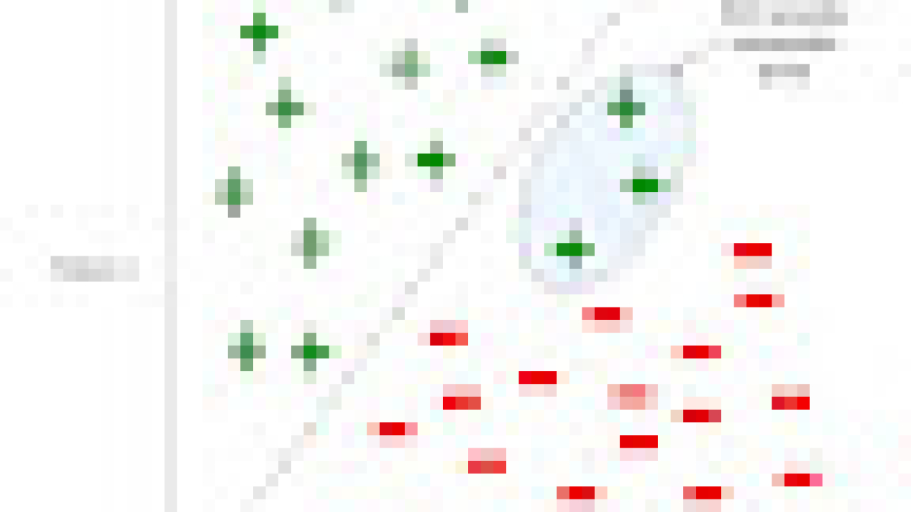
 |
| Figure illustrating the intuitive idea behind RGD in a binary classification setting. Feature 1 and Feature 2 are the features available to the model for predicting the label of a data point. RGD upweights the data points with high losses that have been misclassified by the model. |
We present empirical results comparing RGD with state-of-the-art techniques on standard supervised learning and domain adaptation (refer to the paper for results on meta learning). In all our experiments, we tune the clipping level and the learning rate of the optimizer using a held-out validation set.
We evaluate RGD on several supervised learning tasks, including language, vision, and tabular classification. For the task of language classification, we apply RGD to the BERT model trained on the General Language Understanding Evaluation (GLUE) benchmark and show that RGD outperforms the BERT baseline by +1.94% with a standard deviation of 0.42%. To evaluate RGD’s performance on vision classification, we apply RGD to the ViT-S model trained on the ImageNet-1K dataset, and show that RGD outperforms the ViT-S baseline by +1.01% with a standard deviation of 0.23%. Moreover, we perform hypothesis tests to confirm that these results are statistically significant with a p-value that is less than 0.05.
 |
| RGD’s performance on language and vision classification using GLUE and Imagenet-1K benchmarks. Note that MNLI, QQP, QNLI, SST-2, MRPC, RTE and COLA are diverse datasets which comprise the GLUE benchmark. |
For tabular classification, we use MET as our baseline, and consider various binary and multi-class datasets from UC Irvine’s machine learning repository. We show that applying RGD to the MET framework improves its performance by 1.51% and 1.27% on binary and multi-class tabular classification, respectively, achieving state-of-the-art performance in this domain.
 |
 |
| Performance of RGD for classification of various tabular datasets. |
To evaluate RGD’s generalization capabilities, we use the standard DomainBed benchmark, which is commonly used to study a model’s out-of-domain performance. We apply RGD to FRR, a recent approach that improved out-of-domain benchmarks, and show that RGD with FRR performs an average of 0.7% better than the FRR baseline. Furthermore, we confirm with hypothesis tests that most benchmark results (except for Office Home) are statistically significant with a p-value less than 0.05.
 |
| Performance of RGD on DomainBed benchmark for distributional shifts. |
To demonstrate that models learned using RGD perform well despite class imbalance, where certain classes in the dataset are underrepresented, we compare RGD’s performance with ERM on long-tailed CIFAR-10. We report that RGD improves the accuracy of baseline ERM by an average of 2.55% with a standard deviation of 0.23%. Furthermore, we perform hypothesis tests and confirm that these results are statistically significant with a p-value of less than 0.05.
 |
| Performance of RGD on the long-tailed Cifar-10 benchmark for class imbalance domain. |
The RGD algorithm was developed using popular research datasets, which were already curated to remove corruptions (e.g., noise and incorrect labels). Therefore, RGD may not provide performance improvements in scenarios where training data has a high volume of corruptions. A potential approach to handle such scenarios is to apply an outlier removal technique to the RGD algorithm. This outlier removal technique should be capable of filtering out outliers from the mini-batch and sending the remaining points to our algorithm.
RGD has been shown to be effective on a variety of tasks, including out-of-domain generalization, tabular representation learning, and class imbalance. It is simple to implement and can be seamlessly integrated into existing algorithms with just two lines of code change. Overall, RGD is a promising technique for boosting the performance of DNNs, and could help push the boundaries in various domains.
The paper described in this blog post was written by Ramnath Kumar, Arun Sai Suggala, Dheeraj Nagaraj and Kushal Majmundar. We extend our sincere gratitude to the anonymous reviewers, Prateek Jain, Pradeep Shenoy, Anshul Nasery, Lovish Madaan, and the numerous dedicated members of the machine learning and optimization team at Google Research India for their invaluable feedback and contributions to this work.
 For Google’s 25th birthday, Google.org is providing $10 million in grant funding to support robotics programs and AI education.Read More

 A round-up of our top 10 AI moments of the last 25 years.Read More


The human brain is perhaps the most computationally complex machine in existence, consisting of networks of billions of cells. Researchers currently don’t understand the full picture of how glitches in its network machinery contribute to mental illnesses and other diseases, such as dementia. However, the emerging connectomics field, which aims to precisely map the connections between every cell in the brain, could help solve that problem. While maps have only been created for simpler organisms, technological advances for mapping even larger brains can enable us to understand how the human brain works, and how to treat brain diseases.
Today, we’re excited to announce that the Connectomics team at Google Research and our collaborators are launching a $33 million project to expand the frontiers of connectomics over the next five years. Supported by the Brain Research Through Advancing Innovative Neurotechnologies (BRAIN) Initiative at the National Institutes of Health (NIH) and led by researchers at Harvard University, we’ll be working alongside a multidisciplinary team of experts from the Allen Institute, MIT, Cambridge University, Princeton University and Johns Hopkins University, with advisers from HHMI’s Janelia Research Campus. Our project goal is to tackle an immense challenge in neuroscience: mapping a tiny fraction (2-3%) of the mouse brain. We will specifically target the hippocampal region, which is responsible for encoding memories, attention and spatial navigation. This project is one of 11 funded by the NIH’s $150 million BRAIN Initiative Connectivity Across Scales (BRAIN CONNECTS) program. Google Research is contributing computational and analytical resources to this effort, and will not receive any funding from the NIH. Our project asks a critical question: Can we scale and speed up our technologies enough to map the whole connectome of a mouse brain?
This effort to map the connectome of a small part of the mouse brain builds on a decade of innovation in the field, including many advances initiated by the Connectomics team at Google Research. We hope to accomplish something similar to the early days of the Human Genome Project, when scientists worked for years to sequence a small portion of the human genome as they refined technologies that would enable them to complete the rest of the genome.
In 2021, we and collaborators at Harvard successfully mapped one cubic millimeter of the human brain, which we released as the H01 dataset, a resource for studying the human brain and scaling connectomics technologies. But mapping the entire human brain connectome would require gathering and analyzing as much as a zettabyte of data (one billion terabytes), which is beyond the current capabilities of existing technologies.
Analyzing a mouse connectome is the next best thing. It is small enough to be technically feasible and could potentially deliver insights relevant to our own minds; neuroscientists already use mice to study human brain function and dysfunction. By working together to map 10–15 cubic mm of the mouse brain, we hope to develop new approaches that will allow us to map the entire remainder of the mouse brain, and the human brain thereafter.
 |
| Neuroscientists have been working for decades to map increasingly larger and more complicated connectomes. |
In this connectomics project, we will map the connectome of the hippocampal formation of the mouse brain, which converts short-term memories into long-term memories and helps the mouse navigate in space. The mouse hippocampal formation is the largest area of any brain we’ve attempted to understand in this way. Through mapping this region of the mouse brain, we will create one of the largest datasets in biology, combining about 25,000 terabytes, or 25 petabytes of brain data. For reference, there are about 250 billion stars in our Milky Way Galaxy. If each of those stars was a single byte, it would take 100,000 Milky Way Galaxies to match the 25 petabytes of data that the project will collect when mapping a small region of the mouse brain.
To illustrate the hippocampal project’s scale, we calculated the number of Pixel phones (shown as stacks of Pixels below) needed to store the image data from the completed connectome projects that mapped the roundworm and fruit fly brains, as well as for the mouse hippocampal region and entire mouse brain projects, which are just getting started.
Then, we compared the heights of each Pixel stack to familiar objects and landmarks. It would take a stack of 100 Pixels, as tall as a four-year-old girl, to store the image data for the fruit fly brain, the largest completed project thus far. In contrast, the mouse hippocampal connectome effort will require storage equivalent to more than 48,800 Pixels, reaching as high as the Empire State Building. The animation below shows how the mouse hippocampal project will surpass the scale of previous connectome projects.
 |
| We are partnering with several collaborators to build a connectome (a map of the connections between brain cells) for the hippocampal region of a mouse brain. This project will create the largest connectomic dataset ever, surpassing the scale of previous projects that mapped the smaller roundworm and fruit fly brains. We hope this effort will lead to the development of new approaches that will allow us to later map an entire mouse brain. This animation shows how the field of connectomics is scaling up by calculating the number of Pixel phones needed to store the data from various projects. It would take just two Pixels, the height of an olive, to store the roundworm connectome data, while it would take a stack of Pixels the size of Mount Everest to store the data from an entire mouse connectome. |
Understanding the connectome of the mouse hippocampal formation could help illuminate the way our own brains work. For instance, we may find common features between this circuitry in the mouse brain and human brains that explain how we know where we are, how our brains associate memories with specific locations, and what goes wrong in people who can’t properly form new spatial memories.
Over the last decade, our team has worked to develop tools for managing massive connectomic datasets, and extracting scientific value from them. But a mouse brain has 1,000 times more neurons than the brain of the Drosophila fruit fly, an organism for which we helped build a connectome for a large part of the brain. Starting the mouse brain connectome will challenge us to improve existing technologies to enable us to map more data faster than ever before.
We’ll continue to refine our flood-filling networks, which use deep learning to trace, or “segment”, each neuron’s path through three-dimensional brain volumes made from electron microscope data. We’ll also extend the capabilities of our self-supervised learning technology, SegCLR, which allows us to automatically extract key insights from segmented volumes, such as identifying cell type (e.g., pyramidal neuron, basket neuron, etc.) and parts of each neuron (e.g., axon, dendrite, etc.).
 |
| A flood filling network traces a neuron through three-dimensional brain space. |
We will also continue to enhance the scalability and performance of our core connectomics infrastructure, such as TensorStore for storage and Neuroglancer for visualization, in order to enable all of our computational pipelines and human analysis workflows to operate at these new scales of data. We’re eager to get to work to discover what peering into a mouse’s mind might tell us about our own.
The mouse connectomics project described in this blog post will be supported in part by the NIH BRAIN Initiative under award number 1UM1NS132250. Google Research is contributing computational and analytical resources to the mouse connectome project, and will not receive funding from the NIH. Many people were involved in the development of the technologies that make this project possible. We thank our long-term academic collaborators in the Lichtman Lab (Harvard University), HHMI Janelia, and the Denk Lab (Max Planck Institute for Biological Intelligence), and acknowledge core contributions from the Connectomics Team at Google. We also thank John Guilyard for creating the illustrative animation in this post, and Elise Kleeman, and Erika Check Hayden for their support. Thanks to Lizzie Dorfman, Michael Brenner, Jay Yagnik and Jeff Dean for their support, coordination and leadership.
 Last week at the inaugural Africa Climate Summit (ACS) in Nairobi, Kenya, we joined African leaders and shared our commitment to advance AI solutions to address the clim…Read More


Large language models (LLMs) have enabled a new data-efficient learning paradigm wherein they can be used to solve unseen new tasks via zero-shot or few-shot prompting. However, LLMs are challenging to deploy for real-world applications due to their sheer size. For instance, serving a single 175 billion LLM requires at least 350GB of GPU memory using specialized infrastructure, not to mention that today’s state-of-the-art LLMs are composed of over 500 billion parameters. Such computational requirements are inaccessible for many research teams, especially for applications that require low latency performance.
To circumvent these deployment challenges, practitioners often choose to deploy smaller specialized models instead. These smaller models are trained using one of two common paradigms: fine-tuning or distillation. Fine-tuning updates a pre-trained smaller model (e.g., BERT or T5) using downstream manually-annotated data. Distillation trains the same smaller models with labels generated by a larger LLM. Unfortunately, to achieve comparable performance to LLMs, fine-tuning methods require human-generated labels, which are expensive and tedious to obtain, while distillation requires large amounts of unlabeled data, which can also be hard to collect.
In “Distilling Step-by-Step! Outperforming Larger Language Models with Less Training Data and Smaller Model Sizes”, presented at ACL2023, we set out to tackle this trade-off between model size and training data collection cost. We introduce distilling step-by-step, a new simple mechanism that allows us to train smaller task-specific models with much less training data than required by standard fine-tuning or distillation approaches that outperform few-shot prompted LLMs’ performance. We demonstrate that the distilling step-by-step mechanism enables a 770M parameter T5 model to outperform the few-shot prompted 540B PaLM model using only 80% of examples in a benchmark dataset, which demonstrates a more than 700x model size reduction with much less training data required by standard approaches.
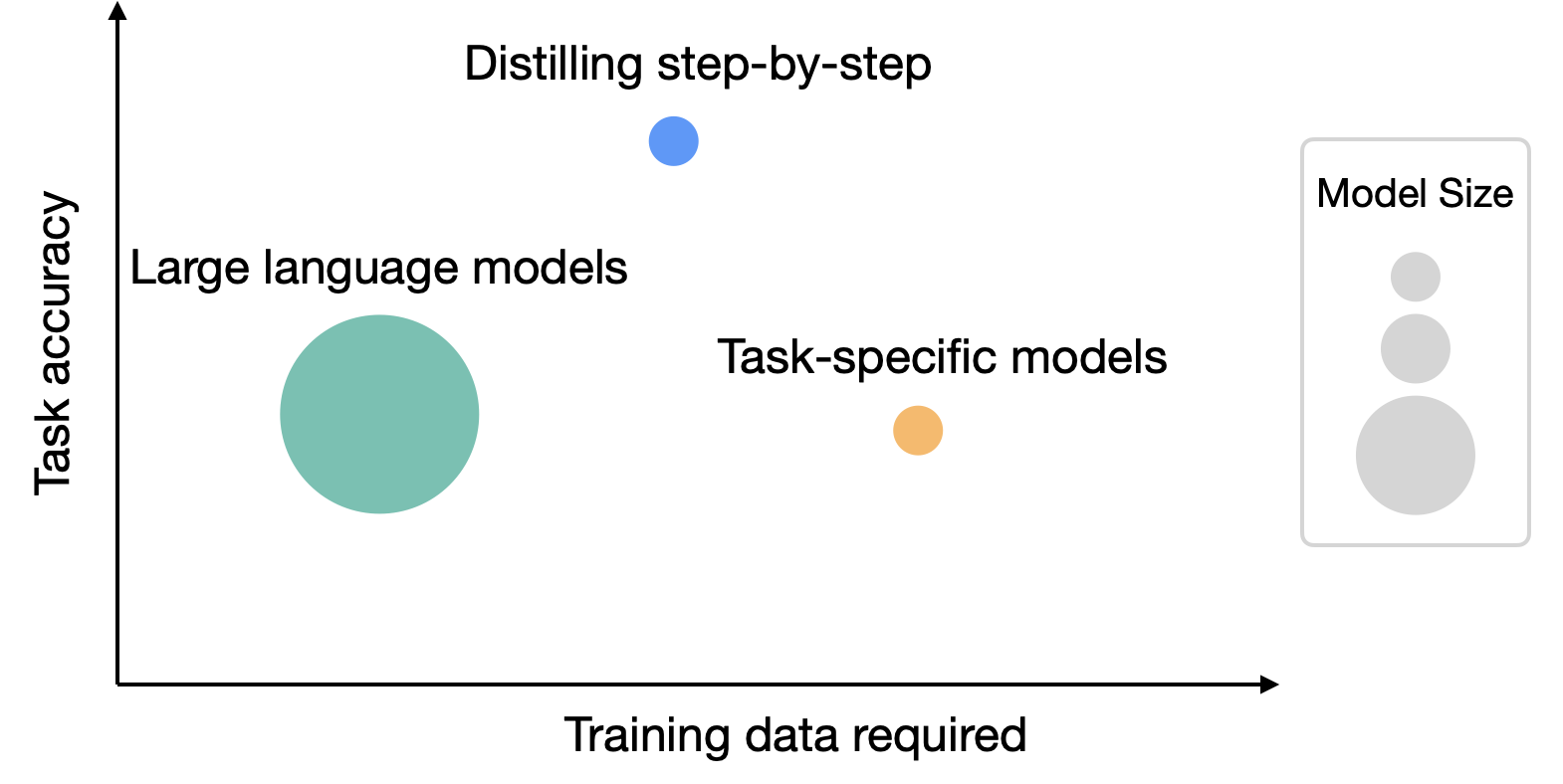 |
| While LLMs offer strong zero and few-shot performance, they are challenging to serve in practice. On the other hand, traditional ways of training small task-specific models require a large amount of training data. Distilling step-by-step provides a new paradigm that reduces both the deployed model size as well as the number of data required for training. |
The key idea of distilling step-by-step is to extract informative natural language rationales (i.e., intermediate reasoning steps) from LLMs, which can in turn be used to train small models in a more data-efficient way. Specifically, natural language rationales explain the connections between the input questions and their corresponding outputs. For example, when asked, “Jesse’s room is 11 feet long and 15 feet wide. If she already has 16 square feet of carpet, how much more carpet does she need to cover the whole floor?”, an LLM can be prompted by the few-shot chain-of-thought (CoT) prompting technique to provide intermediate rationales, such as, “Area = length * width. Jesse’s room has 11 * 15 square feet.” That better explains the connection from the input to the final answer, “(11 * 15 ) – 16”. These rationales can contain relevant task knowledge, such as “Area = length * width”, that may originally require many data for small models to learn. We utilize these extracted rationales as additional, richer supervision to train small models, in addition to the standard task labels.
 |
| Overview on distilling step-by-step: First, we utilize CoT prompting to extract rationales from an LLM. We then use the generated rationales to train small task-specific models within a multi-task learning framework, where we prepend task prefixes to the input examples and train the model to output differently based on the given task prefix. |
Distilling step-by-step consists of two main stages. In the first stage, we leverage few-shot CoT prompting to extract rationales from LLMs. Specifically, given a task, we prepare few-shot exemplars in the LLM input prompt where each example is composed of a triplet containing: (1) input, (2) rationale, and (3) output. Given the prompt, an LLM is able to mimic the triplet demonstration to generate the rationale for any new input. For instance, in a commonsense question answering task, given the input question “Sammy wanted to go to where the people are. Where might he go? Answer Choices: (a) populated areas, (b) race track, (c) desert, (d) apartment, (e) roadblock”, distilling step-by-step provides the correct answer to the question, “(a) populated areas”, paired with the rationale that provides better connection from the question to the answer, “The answer must be a place with a lot of people. Of the above choices, only populated areas have a lot of people.” By providing CoT examples paired with rationales in the prompt, the in-context learning ability allows LLMs to output corresponding rationales for future unseen inputs.
 |
| We use the few-shot CoT prompting, which contains both an example rationale (highlighted in green) and a label (highlighted in blue), to elicit rationales from an LLM on new input examples. The example is from a commonsense question answering task. |
After the rationales are extracted, in the second stage, we incorporate the rationales in training small models by framing the training process as a multi-task problem. Specifically, we train the small model with a novel rationale generation task in addition to the standard label prediction task. The rationale generation task enables the model to learn to generate the intermediate reasoning steps for the prediction, and guides the model to better predict the resultant label. We prepend task prefixes (i.e., [label] and [rationale] for label prediction and rationale generation, respectively) to the input examples for the model to differentiate the two tasks.
In the experiments, we consider a 540B PaLM model as the LLM. For task-specific downstream models, we use T5 models. For CoT prompting, we use the original CoT prompts when available and curate our own examples for new datasets. We conduct the experiments on four benchmark datasets across three different NLP tasks: e-SNLI and ANLI for natural language inference; CQA for commonsense question answering; and SVAMP for arithmetic math word problems. We include two sets of baseline methods. For comparison to few-shot prompted LLMs, we compare to few-shot CoT prompting with a 540B PaLM model. In the paper, we also compare standard task-specific model training to both standard fine-tuning and standard distillation. In this blogpost, we will focus on the comparisons to standard fine-tuning for illustration purposes.
Compared to standard fine-tuning, the distilling step-by-step method achieves better performance using much less training data. For instance, on the e-SNLI dataset, we achieve better performance than standard fine-tuning when using only 12.5% of the full dataset (shown in the upper left quadrant below). Similarly, we achieve a dataset size reduction of 75%, 25% and 20% on ANLI, CQA, and SVAMP.
 |
| Distilling step-by-step compared to standard fine-tuning using 220M T5 models on varying sizes of human-labeled datasets. On all datasets, distilling step-by-step is able to outperform standard fine-tuning, trained on the full dataset, by using much less training examples. |
Compared to few-shot CoT prompted LLMs, distilling step-by-step achieves better performance using much smaller model sizes. For instance, on the e-SNLI dataset, we achieve better performance than 540B PaLM by using a 220M T5 model. On ANLI, we achieve better performance than 540B PaLM by using a 770M T5 model, which is over 700X smaller. Note that on ANLI, the same 770M T5 model struggles to match PaLM’s performance using standard fine-tuning.
 |
| We perform distilling step-by-step and standard fine-tuning on varying sizes of T5 models and compare their performance to LLM baselines, i.e., Few-shot CoT and PINTO Tuning. Distilling step-by-step is able to outperform LLM baselines by using much smaller models, e.g., over 700× smaller models on ANLI. Standard fine-tuning fails to match LLM’s performance using the same model size. |
Finally, we explore the smallest model sizes and the least amount of data for distilling step-by-step to outperform PaLM’s few-shot performance. For instance, on ANLI, we surpass the performance of the 540B PaLM using a 770M T5 model. This smaller model only uses 80% of the full dataset. Meanwhile, we observe that standard fine-tuning cannot catch up with PaLM’s performance even using 100% of the full dataset. This suggests that distilling step-by-step simultaneously reduces the model size as well as the amount of data required to outperform LLMs.
 |
| We show the minimum size of T5 models and the least amount of human-labeled examples required for distilling step-by-step to outperform LLM’s few-shot CoT by a coarse-grained search. Distilling step-by-step is able to outperform few-shot CoT using not only much smaller models, but it also achieves so with much less training examples compared to standard fine-tuning. |
We propose distilling step-by-step, a novel mechanism that extracts rationales from LLMs as informative supervision in training small, task-specific models. We show that distilling step-by-step reduces both the training dataset required to curate task-specific smaller models and the model size required to achieve, and even surpass, a few-shot prompted LLM’s performance. Overall, distilling step-by-step presents a resource-efficient paradigm that tackles the trade-off between model size and training data required.
Distilling step-by-step is available for private preview on Vertex AI. If you are interested in trying it out, please contact vertex-llm-tuning-preview@google.com with your Google Cloud Project number and a summary of your use case.
This research was conducted by Cheng-Yu Hsieh, Chun-Liang Li, Chih-Kuan Yeh, Hootan Nakhost, Yasuhisa Fujii, Alexander Ratner, Ranjay Krishna, Chen-Yu Lee, and Tomas Pfister. Thanks to Xiang Zhang and Sergey Ioffe for their valuable feedback.