The International Conference on Robotics and Automation (ICRA) 2020 is being hosted virtually from May 31 – Jun 4.
We’re excited to share all the work from SAIL that’s being presented, and you’ll find links to papers, videos and blogs below. Feel free to reach out to the contact authors directly to learn more about the work that’s happening at Stanford!
Authors: Margaret M. Coad, Laura H. Blumenschein, Sadie Cutler, Javier A. Reyna Zepeda, Nicholas D. Naclerio, Haitham El-Hussieny, Usman Mehmood, Jee-Hwan Ryu, Elliot W. Hawkes, and Allison M. Okamura
We projected head-dependent pairs from both English (light colors) and French (dark colors) into a syntactic space trained on solely English mBERT representations. Both English and French head-dependent vectors cluster; dependencies of the same label in both English and French share the same cluster. Although our method has no access to dependency labels, the dependencies exhibit cross-lingual clustering that largely agree with linguists’ categorizations.
If you ask a deep neural network to read a large number of languages, does it share what it’s learned about sentence structure between different languages?
Deep neural language models like BERT have recently demonstrated a fascinating level of understanding of human language. Multilingual versions of these models, like Multilingual BERT (mBERT), are able to understand a large number of languages simultaneously. To what extent do these models share what they’ve learned between languages?
Focusing on the syntax, or grammatical structure, of these languages, we show that Multilingual BERT is able to learn a general syntactic structure applicable to a variety of natural languages. Additionally, we find evidence that mBERT learns cross-lingual syntactic categories like “subject” and “adverb”—categories that largely agree with traditional linguistic concepts of syntax! Our results imply that simply by reading a large amount of text, mBERT is able to represent syntax—something fundamental to understanding language—in a way that seems to apply across many of the languages it comprehends.
More specifically, we present the following:
We apply the structural probe method of Hewitt and Manning (2019) to 10 languages, finding syntactic subspaces in a multilingual setting.
Through zero-shot transfer experiments, we demonstrate that mBERT represents some syntactic features in syntactic subspaces that overlap between languages.
Through an unsupervised method, we find that mBERT natively represents dependency clusters that largely overlap with the UD standard.
If you’d like to skip the background and jump to the discussion of our methods, click here. Otherwise, read on!
Learning Languages
Past childhood, humans usually learn a language by comparison to one we already speak.1 We naturally draw parallels between sentences with similar meanings—for example, after learning some French, one can work out that Je vis le chat mignon is essentially a word-for-word translation of I see the cute cat. Importantly, humans draw parallels in syntax, or the way words are organized to form meaning; most bilinguals know that mignon is an adjective which describes the noun chat, just as cute describes the noun cat—even though the words are in the opposite order between languages.
How do we train a neural network to understand multiple languages at the same time? One intuitive approach might be to equip the neural network with a multilingual dictionary and a list of rules to transfer between one language to another. (For example, adjectives come before the noun in English but after the noun in Khmer.) However, mirroring recent developments in monolingual neural networks, one more recent method is to give our neural network enormous amounts of data in multiple languages. In this approach, we never provide even a single translation pair, much less a dictionary or grammar rules.
Surprisingly, this trial by fire works! A network trained this way, like Google’s Multilingual BERT, is able to understand a vast number of languages beyond what any human can handle, even a typologically divergent set ranging from English to Hindi to Indonesian.
This raises an interesting question: how do these networks understand multiple languages at the same time? Do they learn each language separately, or do they draw parallels between the way syntax works in different languages?
Knowing What it Means to “Know”
First, let’s ask: what does it even mean for a neural network to “understand” a linguistic property?
One way to evaluate this is through the network’s performance on a downstream task, such as a standard leaderboard like the GLUE (General Language Understanding Evaluation) benchmark. By this metric, large models like BERT do pretty well! However, although high performance numbers suggest in some sense that the model understands some aspects of language generally speaking, they conflate the evaluation of many different aspects of language, and it’s difficult to test specific hypotheses about the individual properties of our model.
Instead, we use a method known as probing. The central idea is as follows: we feed linguistic data for which we know the property we’re interested in exploring (e.g. part-of-speech) through the network we want to probe. Instead of looking at the predictions of the model themselves, for each sentence we feed through, we save the hidden representations, which one can think of as the model’s internal data structures. We then train a probe—a secondary model—to recover the target property from these representations, akin to how a neuroscientist might read out emotions from a MRI scan of your brain.
Probes are usually designed to be simple, to test what the neural network makes easily accessible. intuitively, the harder we try to tease a linguistic property out of the representations, the less the representations themselves matter to your final results. As an example, we might be able to build an extremely complex model to predict whether someone is seeing a cat, based on the raw data coming from the retina; however, this doesn’t mean that the retina itself intrinsically “understands” what a cat is.2
A Tale of Syntax and Subspaces
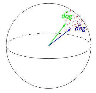
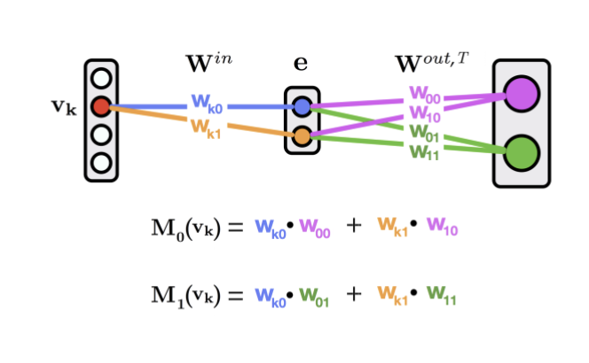
So what form, exactly, do these hidden representations take? The innards of a neural network like BERT represent each sentence as a series of real-valued vectors (in real life, these are 768-dimensional, but we’ve represented them as three-dimensional here):
A probe, then, is a model that maps from a word vector to some linguistic property of interest. For something like part of speech, this might take the form of a 1-layer neural classifier which predicts a category (like noun or verb).
But how do we evaluate whether a neural network knows something as nebulous as syntax, the way words and phrases are arranged to create meaning? Linguists believe sentences are implicitly organized into syntax trees, which we generate mentally in order to produce a sentence. Here’s an example of what that looks like:
Syntax tree for French Jean qui avait faim joue bien dans le jardin (Jean, who was hungry, plays in the garden).
To probe whether BERT encodes a syntax tree internally, we apply the structural probe method [Hewitt and Manning, 2019]. This finds a linear transformation3 such that the tree constructed by connecting each word to the word closest to it approximates a linguist’s idea of what the parse tree should look like. This ends up looking like this:
Intuitively, we can think of BERT vectors as lying in a 768-dimensional space; the structural probe tries to find a linear subspace of the BERT space which best recovers syntax trees.
Does this work, you might ask? Well, this certainly seems to be the case:
A gold parse tree annotated by a linguist, and a parse tree generated from Monolingual BERT embeddings. From Coenen et al. (2019).
Hewitt and Manning apply this method only to monolingual English BERT; we apply their method to 10 other languages, finding that mBERT encodes syntax to various degrees in all of them. Here’s a table of performance (measured in UUAS, or unlabeled undirected accuracy score) as graphed against the rank of the probe’s linear transformation:
Probing for Cross-Lingual Syntax
With this in mind, we can turn to the question with which we started this blog post:
Does Multilingual BERT represent syntax similarly cross-lingually?
To answer this, we train a structural probe to predict syntax from representations in one language—say, English—and evaluate it on another, like French. If a probe trained on mBERT’s English representations performs well when evaluated on French data, this intuitively suggests that the way mBERT encodes English syntax is similar to the way it encodes French syntax.
Does this work? In a word, basically:
Syntactic trees for a single English sentence generated by structural probes trained on English, French, and Indonesian data.
Black represents the reference syntactic tree as defined by a linguist.
The English structural probe is almost entirely able to replicate the syntactic tree, with one error;
the French probe finds most of the syntactic tree, while the Indonesian probe is able to recover the high-level structure but misses low-level details.
Out of the 11 languages that we evaluate on, we find that probes trained on representations from one language are able to successfully recover syntax trees—to varying degrees—in data from another language. Evaluated on two numerical metrics of parse tree accuracy, applying probes cross-lingually performs surprisingly well! This performance suggests that syntax is encoded similarly in mBERT representations across many different languages.
UUAS
DSpr.
Best baseline
0%
0%
Transfer from best source language
62.3%
73.1%
Transfer from holdout subspace (trained on all languages other than eval)
70.5%
79%
Transfer from subspace trained on all languages (including eval)
88.0%
89.0%
Training on evaluation language directly
100%
100%
Table: Improvement for various transfer methods over best baseline, evaluated on two metrics: UUAS (unlabeled undirected accuracy score) and DSpr. (Spearman correlation of tree distances). Percent improvement is calculated with respect to the total possible improvement in recovering syntactic trees over baseline (as represented by in-language supervision.)
Finding Universal Grammatical Relations in mBERT
We’ve shown that cross-lingual syntax exists—can we visualize it?
Recall that the structural probe works by finding a linear subspace optimized to encode syntax trees. Intuitively, this syntactic subspace might focus on syntactic aspects of mBERT’s representations. Can we visualize words in this subspace and get a first-hand view of how mBERT represents syntax?
One idea is to focus on the edges of our syntactic tree, or head-dependent pairs. For example, below, was is the head of the dependent chef:
Let’s try to visualize these vectors in the syntactic subspace and see what happens! Define the head-dependent vector as the vector between the head and the dependent in the syntactic subspace:
We do this for every head-dependent pair in every sentence in our corpus, then visualize the resulting 32-dimensional vectors in two dimensions using t-SNE, a dimensionality reduction algorithm. The results are striking: the dependencies naturally separate into clusters, whose identities largely overlap with the categories that linguists believe are fundamental to language! In the image below, we’ve highlighted the clusters with dependency labels from Universal Dependencies, like amod (adjective modifying a noun) and conj (two clauses joined by a coordinating conjunction like and, or):
Importantly, these categories are multilingual. In the above diagram, we’ve projected head-dependent pairs from both English (light colors) and French (dark colors) into a syntactic space trained on solely English mBERT representations. We see that French head-dependent vectors cluster as well, and that dependencies with the same label in both English and French share the same cluster.
Freedom from Human-Chosen Labels
The fact that BERT “knows” dependency labels is nothing new; previous studies have shown high accuracy in recovering dependency labels from BERT embeddings. So what’s special about our method?
Training a probe successfully demonstrates that we can map from mBERT’s representations to a standard set of dependency category labels. But because our probe needs supervision on a labeled dataset, we’re limited to demonstrating the existence of a mapping to human-generated labels. In other words, probes make it difficult to gain insight into the categories drawn by mBERT itself.
By contrast, the structural probe never receives information about what humans think dependency label categories should look like. Because we only ever pass in head-dependent pairs, rather than the category labels associated with these pairs, our method is free from human category labels. Instead, the clusters that emerge from the data are a view into mBERT’s innate dependency label representations.4
Taking a closer look, what can we discover about how mBERT categorizes head-dependency relations, as compared to human labels? Our results show that mBERT draws slightly different distinctions from Universal Dependencies. Some are linguistically valid distinctions not distinguished by the UD standards, while others are more influenced by word order, separating relations that most linguists would group together. Here’s a brief overview:
t-SNE visualization of 100,000 syntactic difference vectors projected into the cross-lingual syntactic subspace of Multilingual BERT. We exclude `punct` and visualize the top 11 dependencies remaining, which are collectively responsible for 79.36% of the dependencies in our dataset. Clusters of interest highlighted in yellow; linguistically interesting clusters labeled.
Adjectives: We find that mBERT breaks adjectives into two categories: prenominal adjectives in cluster (b) (e.g., Chinese 獨特的地理) and postnominal adjectives in cluster (u) (e.g., French applicationsdomestiques).
Nominal arguments: mBERT maintains the UD distinction between subject and object. However, indirect objects cluster with direct objects; other adjuncts cluster with subjects if near the beginning of a sentence and obj otherwise. This suggests that mBERT categorizes nominal arguments into pre-verbal and post-verbal categories.
Relative clauses In the languages in our dataset, there are two major ways of forming relative clauses. Relative pronouns (e.g., English the manwhois hungry are classed by Universal Dependencies as being an nsubj dependent, while subordinating markers (e.g., English I knowthatshe saw me) are classed as the dependent of a mark relation. However, mBERT groups both of these relations together, clustering them distinctly from most nsubj and mark relations.
Determiners The linguistic category of determiners (det) is split into definite articles (i), indefinite articles (e), possessives (f), and demonstratives (g). Sentence-initial definite articles (k) cluster separately from other definite articles (j).
Expletive subjects Just as in UD, expletive subjects, or third person pronouns with no syntactic meaning (e.g. English Itis cold, French Ilfaudrait, Indonesian Yangmenjadi masalah kemudian), cluster separately (k) from other nsubj relations (small cluster in the bottom left).
Conclusion
In this work, we’ve found that BERT shares some of the ways it represents syntax between its internal representations of different languages. We’ve provided evidence that mBERT learns natural syntactic categories that overlap cross-lingually. Interestingly, we also find evidence that these categories largely agree with traditional linguistic concepts of syntax.
Excitingly, our methods allow us to examine fine-grained syntactic categories native to mBERT. By removing assumptions on what the ontology of syntactic relations should look like, we discover that mBERT’s internal representations innately share significant overlap with linguists’ idea of what syntax looks like. However, there are also some interesting differences between the two, the nature of which is definitely worth further investigation!
If you’d like to run some tests or generate some visualizations of your own, please head on over to the multilingual-probing-visualization codebase!
Finally, I’m deeply grateful to John Hewitt and Chris Manning, as well as members of the Stanford NLP group for their advice, including but not limited to: Erik Jones, Sebastian Schuster, and Chris Donahue. Many thanks also to John Hewitt and Dylan Losey for reading over the draft of this blog post, and to Mohammad Rasooli for advice on Farsi labels in the original paper.
For a linguistic perspective (specifically, in the field of second-language acquisition), see Cook (1995). ↩
This definition is a general overview and leaves some important questions. How exactly, for instance, do we evaluate the complexity of our probe? Relatedly, how much of the performance improvement is due to the model, and how much is due to the probe itself? For more work on this, see Hewitt and Liang (2019) and Pimentel et al. (2020). ↩
A linear transformation on a vector is simply multiplication by a matrix: ↩
Technically speaking, this is constrained to the assumption that BERT would choose the same head-dependent pairs as UD does. ↩
Sound, smell, taste, touch, and vision – these are the five senses that humans use to perceive and understand the world. We are able to seamlessly combine these different senses when perceiving the world. For example, watching a movie requires constant processing of both visual and auditory information, and we do that effortlessly. As roboticists, we are particularly interested in studying how humans combine our sense of touch and our sense of sight. Vision and touch are especially important when doing manipulation tasks that require contact with the environment, such as closing a water bottle or inserting a dollar bill into a vending machine.
Let’s take closing a water bottle as an example. With our eyes, we can observe the colors, edges, and shapes in the scene, from which we can infer task-relevant information, such as the poses and geometry of the water bottle and the cap. Meanwhile, our sense of touch tells us texture, pressure, and force, which also give us task-relevant information such as the force we are applying to the water bottle and the slippage of the bottle cap in our grasp. Furthermore, humans can infer the same kind of information using either or both types of senses: our tactile senses can also give us pose and geometric information, while our visual senses can predict when we are going to make contact with the environment.
Humans use visual and tactile senses to infer task-relevant information and actions for contact-rich tasks, such as closing a bottle.
From these multimodal observations and task-relevant features, we come up with appropriate actions for the given observations to successfully close the water bottle. Given a new task, such as inserting a dollar into a vending machine, we might use the same task-relevant information (poses, geometry, forces, etc) to learn a new policy. In other words, there are certain task-relevant multimodal features that generalize across different types of tasks.
Learning features from raw observation inputs (such as RGB images and force/torque data from sensors commonly seen on modern robots) is also known as representation learning. We want to learn a representation for vision and touch, and preferably a representation that can combine the two senses together. We hypothesize that if we can learn a representation that captures task-relevant features, we can use the same representation for similar contact-rich tasks. In other words, learning a rich multimodal representation can help us generalize.
While humans interact with the world in an inherently multimodal manner, it is not clear how to combine very different kinds of data directly from sensors. RGB images from cameras are very high dimensional (often around 640 x 480 x 3 pixels). On the other hand, force/torque sensor readings only have 6 dimensions but also have the complicating quality of sometimes rapidly changing (e.g. when the robot is not touching anything, the sensor registers 0 newtons, but that can quickly jump to 20 newtons once contact is made).
Combining Vision and Touch
How do we combine vision and touch when they have such different characteristics?
Our encoder architectures to fuse the multimodal inputs.
We can leverage a deep neural network to learn features from our high dimensional raw sensor data. The above figure shows our multimodal representation learning neural network architecture, which we train to create a fused vector representation of RGB images, force sensor readings (from a wrist-attached force/torque sensor), and robot states (the position and velocity of the robot wrist from which the peg is attached).
Because our sensor readings have such different characteristics, we use a different network architecture to encode each modality:
-The image encoder is a simplified FlowNet1 network, with a 6-layer convolutional neural network (CNN). This will be helpful for our self-supervised objective.
-Because our force reading is a time series data with temporal correlation, we take the causal convolutions of our force readings. This is similar to the architecture of WaveNet2, which has been shown to work well with time-sequenced audio data.
-For proprioceptive sensor readings (end-effector position and velocity), we encode it with fully connected layers, as this is commonly done in robotics.
Each encoder produces a feature vector. If we want a deterministic representation, we can combine them into one vector by just concatenating them together. If we use a probabilistic representation, where each feature vector actually has a mean vector and a variance vector (assuming Gaussian distributions), we can combine the different modality distributions using the Product of Experts idea of multiplying the densities of the distributions together by weighting each mean with its variance. The resulting combined vector is our multimodal representation.
How do we learn multimodal features without manual labeling?
Our modality encoders have close to half a million learnable parameters, which would require large amounts of labeled data to train with supervised learning. It would be very costly and expensive to manually label our data. However, we can design training objectives whose labels are automatically generated during data collection. In other words, we can train the encoders using self-supervised learning. Imagine trying to annotate 1000 hours of video of a robot doing a task or trying to manually label the poses of the objects. Intuitively, you’d much rather just write down a rule like ‘keep track of the force on the robot arm and label the state and action pair when force readings are too high’, rather than checking each frame one by one for when the robot is touching the box. We do something similar, by algorithmically labeling the data we collect from the robot rollouts.
Our self-supervised learning objectives.
We design two learning objectives that capture the dynamics of the sensor modalities: (i) predicting the optical flow of the robot generated by the action and (ii) predicting whether the robot will make contact with the environment given the action. Since we usually know the geometry, kinematics, and meshes of a robot, ground-truth optical flow annotations can be automatically generated given the joint positions and robot kinematics. Contact prediction can also be automatically generated by looking for spikes in the force sensor data.
Our last self-supervised learning objective attempts to capture the time-locked correlation between the two different sensor modalities of vision and touch, and learn the relationship between them. When a robot touches an environment, a camera captures the interaction and the force sensor captures the contact at the same time. So, this objective predicts whether our input modalities are time aligned. During training, we give our network both time-aligned data and also randomly shifted sensor data. Our network needs to be able to predict from our representation whether the inputs are aligned or not.
To train our model, we collected 100,000 data points in 90 minutes by having the robot perform random actions as well as pre-defined actions that encourage peg insertion and collecting self-supervised labels as described above. Then, we learn our representation via standard stochastic gradient descent, training for 20 epochs.
How do we know if we have a good multimodal representation?
A good representation should:
Enable us to learn a policy that is able to accomplish a contact-rich manipulation task (e.g. a peg insertion task) in a sample-efficient manner
Generalize across task instances (e.g. different peg geometries for peg insertion)
Enable use to learn a policy that is robust to sensor noises, external perturbations, and different goal locations
To study how to learn this multimodal representation, we use a peg insertion task as an experimental setup. Our multimodal inputs are raw RGB image, force readings from a force/torque sensor, and end-effector position and velocity. And unlike classical works on tight tolerance peg insertion that need prior knowledge of peg geometries, we will be learning policies for different geometries directly from raw RGB images and force/torque sensor readings. More importantly, we want to learn a representation from one peg geometry, and see if that representation can generalize to new unseen geometries.
Learning a policy
We want the robot to be able to learn policies directly from its own interactions with the environment. Here, we turn to deep reinforcement learning (RL) algorithms, which enable agents to learn from trial and error and a reward function.
Deep reinforcement learning has shown great advances in playing video games, robotic grasping, and solving Rubik’s cubes. Specifically, we use Trust Region Policy Optimization3, an on-policy RL algorithm, and a dense reward that guides the robot towards the hole for peg insertion.
Once we learn the representation, we feed the representation directly to a RL policy. And we are able to learn a peg insertion task for different peg geometries in about 5 hours from raw sensory inputs.
Here is the robot when it first starts learning the task.
About 100 episodes in (which is 1.5 hours), the robot starts touching the box.
Insert gif episode 100
And in 5 hours, the robot is able to reliably insert the peg for a round peg, triangular peg, and also a semi-circular peg.
Evaluation of our representation
We evaluate how well our representation captures our multimodal sensor inputs by testing how well the representation generalizes to new task instances, how robust our policy is with the representation as state input, and how the different modalities (or lack thereof) affect the representation learning.
Generalization of our representation
We examine the potential of transferring the learned policies and representations to two novel shapes previously unseen in representation and policy training, the hexagonal peg and the square peg. For policy transfer, we take the representation model and the policy trained for the triangular peg, and execute with the new unseen square peg. As you can see in the gif below, when we do policy transfer, our success rate drops from 92% to 62%. This shows that a policy learned for one peg geometry does not necessarily transfer to a new peg geometry.
A better transfer performance can be achieved by taking the representation model trained on the triangular peg, and training a new policy for the new hexagonal peg. As seen in the gif, our peg insertion rate goes up to 92% again when we transfer the multimodal representation. Even though the learned policies do not transfer to new geometries, we show that our multimodal representation from visual and tactile feedback can transfer to new task instances. Our representation generalizes to new unseen peg geometries, and captures task-relevant information across task instances.
Policy robustness
We showed that our policy is robust to sensor noises for the force/torque sensors and for the camera.
Force Sensor Perturbation: When we tap the force/torque sensor, this sometimes tricks the robot to think it is making contact with the environment. But the policy is still able to recover from these perturbations and noises.
Camera Occlusion: When we intermittently occlude the camera after the robot has already made contact with the environment. The policy is still able to find the hole from the robot states, force readings, and the occluded images.
Goal Target Movement: We can move the box to a new location that has never been seen by the robot during training, and our robot is still able to complete the insertion.
External Forces: We can also perturb the robot and apply external forces directly on it, and is it still able to finish the insertion.
Also notice we run our policies on two different robots, the orange KUKA IIWA robot and the white Franka Panda robot, which shows that our method works on different robots.
Ablation study
To study the effects of how the different modalities affect the representation, we ran an ablation study in simulation. In our simulation experiments where we randomize the box location, we can study how each sensor is being used by completely taking away a modality during representation and policy training. If we only have force data, our policy is not able to find the box. With only image data, we achieve a 49% task success rate, but our policy really struggles with aligning the peg with the hole, since the camera cannot capture these small precise movements. With both force and image inputs, our task completion rate goes up to 77% in simulation.
Simulation results for modality ablation study
The learning curves also demonstrate that the Full Model and the Image Only Model (No Haptics) have similar returns in the beginning of the training. As training goes on and the robot learns to get closer to the box, the returns start to diverge when the Full Model is able to more quickly and robustly learn how to insert the peg with both visual and force feedback.
Policy learning curves for modality ablation study
It’s not surprising that learning a representation with more modalities improves policy learning, but our result also shows that our representation and policy are using all the modalities for contact-rich tasks.
Summary
As an overview of our method, we collect self-labeled data through self-supervision, which takes about 90 minutes to collect 100k data points. We can learn a representation from this data, which takes about 24 hours training on a GPU, but is done fully offline. Afterward, you can learn new policies from the same representation, which only takes 5 hours of real robot training. This method can be done on different robots or for different kinds of tasks.
Here are some of the key takeaways from this work. The first is, self-supervision, specifically dynamics and temporal concurrency prediction can give us rich objectives to train a representation model of different modalities.
Second, our representation that captures our modality concurrency and forward dynamics can generalize across task instances (e.g. peg geometries and hole location) and is robust to sensor noise. This suggests that the features from each modality and the relationship between them are useful across different instances of contact rich tasks.
Lastly, our experiments show that learning multimodal representation leads to learning efficiency and policy robustness.
For future work, we want our method to be able to generalize beyond a task family to completely different contact-rich tasks (e.g. chopping vegetables, changing a lightbulb, inserting an electric plug). To do so, we might need to utilize more modalities, such as incorporating temperature, audio, or tactile sensors, and also find algorithms that can give us quick adaptations to new tasks.
This blog post is based on the two following papers:
How do you teach a robot to pack your groceries into different boxes? While modern industrial robots are incredibly capable and precise, they require tremendous expertise to program and are designed to execute the exact same motion millions of times. Trying to program a robot to be able to pick up any kind of groceries, each with different characteristics, geometries, and weight, and pack them in the right boxes, would be incredibly difficult.
In this post, we introduce methods for teaching a robot to learn new tasks by showing a single demonstration of the task. This is also called one-shot imitation learning. To get a better idea of why this is an important problem, let’s first imagine a scenario where a robot is responsible for packaging in the warehouse: It needs to pick up all kinds of items people order from storage and then place the objects in shipping containers. The size of the problem can quickly become intractable if we consider the combination of different objects and different containers. For example, packaging five types of items into five types of shipping containers results in 120 possible combinations. This means that the robot would need to learn 120 different policies to accomplish all the different combinations. Imagine if you had to give instructions to someone to pack your groceries. That seems easy–millions of humans do this every day. But here’s a twist: this robot has never seen a milk carton or a paper bag. And the robot also doesn’t know how to use its arm, so you need to instruct it where to place its hand (close to the milk carton), when to close its hand (when it’s on top of the jug), and how to move the milk to the right paper bag. Now imagine if for every single item and every single bag you needed to give these detailed instructions for this robot. That is how difficult it is to program a robot to do a task that is simple for humans.
But from another perspective, we do know that packaging five types of items into five types of shipping containers is not so complicated; ultimately, it just involves picking up a sequence of objects and putting them into a box. And, we know that picking up and placing different items into the same shipping container is basically the same thing regardless of the item. In other words, we can use the same skill to place different objects into the same container, and consider this a subtask of the full job to be done. We can take this idea further: even picking up different objects is quite similar since moving toward objects is independent of the object type. Based on this insight, we would not have to really write hundreds of entirely different programs to package five items into five containers. Instead, we can focus on implementing primitive skills like grasping, moving, dropping, which can be composed to package items in arbitrary containers.
We introduce a suit of algorithms for learning to imitate from video demonstration by leveraging compositional structures such as neural programs.
In this post, we discuss approaches that aim to leverage the above intuition of compositionality, i.e., generalizing to new tasks by composing pieces of smaller tasks, to reduce the effort robots need to learn new tasks. We refer to structured representations that allow simpler constituents to recombine and form new representations as “compositional priors”. In each section, we gradually build stronger compositional priors into our models and observe its effect on learning efficiency for robotics tasks such as the one above.
We will first define the problem setup and what we mean for robots to learn new tasks, which provides a unified setup for us to evaluate and compare different approaches. Then, we shall discuss the following approaches: (i) Neural Task Programming, (ii) Neural Task Graph Networks, (iii) Continuous Planner. We hope that these more human efforts can translate to more efficient learning of our robots.
The Problem: One-shot Imitation Learning
We mentioned that we hope to leverage compositional prior to improve learning efficiency of robots. It is therefore important that we use a unified setup to compare different approaches. However, there are many ways a robot can learn. It can directly interact with the environment and use trial-and-error to learn actions that can lead to “good” consequences. On the other hand, the robot can also learn new tasks by following demonstrations: an expert, or someone who knows how the task is done, can demonstrate (potentially many times) to the robot how to complete the task. In this post we consider the latter, and constrain the robot to learn from a single demonstration, which is known as one-shot imitation learning.
Humans can learn many things from a single demonstration. For example, if someone wants to learn how to package different items into shipping containers, then all we need is a single demonstration to specify what items should go into what containers. While it seems natural for humans, how can we have agents or robots do the same? One clever approach is to formulate it as another learning problem: we can have the agent ‘learn to learn’, so that it is trained to be able to learn a new task from a single demonstration.
The one-shot imitation learning problem is to have the robots ‘learn to learn’, so that they are trained to be able to learn a new task from a single demonstration.
It is important to differentiate the two types of “learning” here. The first type is a more ordinary one: the learning for an agent to do new tasks like packaging items in a warehouse, i.e. one-shot imitation learning. For this type of learning, the agent always only has a single demonstration without further interaction with the environment in our setting. But remember, the agent does not know how to do this at the outset. So, the second type of learning refers to the agent becoming able to do the first type of learning, i.e. learning how to be able to do a task from a single demonstration well. When we say we would like to improve the “learning efficiency” of our robots or agents, we mean to improve the learning efficiency of this second type of learning: how can we have agents that quickly learn the ability to do new tasks from a single demonstration. We want to improve efficiency of this because providing demonstrations to robotics is fairly time consuming, and if it is necessary to provide millions of such demonstrations for the agent to learn one-shot imitation
Approach 1: Neural Task Programming (NTP)
As we have discussed, we have the intuition that an overall objective (e.g., packaging items) can be decomposed into simpler objectives (e.g., picking certain items) recursively (i.e. subtasks can also be composed of subtasks). This allows us to write robot programs more efficiently since we get to reuse a lot of the smaller pieces for making these programs, and we hope we can apply the same intuition to our one-shot imitation agent so that it can learn to learn new tasks more efficiently.
One may notice that this intuition emulates a typical computer program, 1) invoking a sub-program 2) return to the calling program (return). This is the essence of neural program synthesis, which uses neural networks to simulate computer programs. Neural program synthesis has many advantages over ordinary neural networks, such as learning discrete operations. More details about the model architecture and the idea of neural program synthesis can be found in our paper, its predecessor NPI 1 (Neural Programmer-Interpreter), and seminal works such as Neural Turing Machine 2.
Similarly to the Neural Programmer-Interpreter, Neural Task Programming (NTP) achieves this program-like recursive decomposition by supervised training. Given the current task, we provided the model with the correct decomposition of that task into subtasks, and trained the model to perform this decomposition based on the current state observation and task specification (or demonstration).
NTP core architecture.
In the figure we use the “pick_and_place” as the input program or objective, which we aim to decompose. The module is trained to have four outputs:
The task decomposition; in this case we know “pick_and_place” can be further decomposed to “pick.”
The end-of-program probability or whether to “return” the current program. For example, we can decompose a “pick_and_place” into a “pick” and a “place,” and the “pick_and_place” is complete or can return only if both the “pick” and the “place” are done.
“Task Specification” when invoking a sub-program and continuing with the recursion, in which case we just update the scope of the task specification for the next recursion.
“API Arguments” when invoking a sub-program and we reach the bottom of recursion, in which case we call the robot to execute actual movements and provide the API arguments such as object should the robot arm move to. 2)
This last type of output, which leads to a hierarchical decomposition of task specification/demonstration, is another key factor of NTP. Take “pick_and_place” again as an example. There might be multiple instances of “pick_and_place”s in the full task specification: we pick up different objects and place them onto/into different objects. How does the model know what objects we are currently interested in for this specific “pick_and_place”? The obvious answer is that we should compare the current state observation with the task specification, by which we can figure out the current progress (i.e., what “pick_and_place”s are done) and decide what objects to pick and place. This can be challenging if the task specification is long.
On the other hand, it is more ideal if the NTP program to process “pick_and_place” only sees the part of the specification that is relevant to this specific “pick_and_place”. In this case, we only have to recognize the objects in the clipped specification instead of searching from the full specification. In fact, this clipped specification is all we need to correctly decompose this “pick_and_place.” Therefore, we recursively decompose and update the scope of task specifications as outputs of NTP modules. A long task demonstration thus can be decomposed recursively to shorter clips as the program traverses down the hierarchy. In more technical terms, the hierarchical decomposition of demonstrations prevents the model from learning spurious dependencies on training data, resulting in better reusability of each program. Below is an example showing how NTP hierarchically decomposes a complex long-horizon task.
A sample block stacking task neural program generated by NTP.
Approach 2: Neural Task Graph Networks (NTG)
Recall that the “learning efficiency” we are interested in is how fast we can train a model so that the model can learn new tasks with a single demonstration. We have introduced NTP, which learns to hierarchically decompose tasks for execution. Our intuition is that it is easier to learn to decompose tasks compared to directly determining what the robot action should be based on an arbitrary task demonstration that can be quite long. In other words, if models can more efficiently learn to decompose tasks, then we can improve our robot’s learning efficiency But the NTP module still has to learn a lot of very complicated tasks all at the same time: what programs to decompose, whether the current program is finished, what are the arguments for the subprograms, how to change the scope of task specification. In addition, a single error at the higher level can propagate and affect all the following decompositions. For example, if the task specification scope for “pick_and_place” is off, then we cannot have the correct scopes for “pick” and “place.”
Therefore, the next approach, Neural Task Graph Networks (NTG) improves over NTP by changing two things to make learning easier. First, we introduce several modules to specialize in different aspects instead of having a single NTP module to learn everything. This modularization more explicitly specifies what each module should learn. Second, task decomposition is explicitly represented with a task graph, which captures all the possible ways to complete a task. This is in contrast to NTP, which trains the agent to decompose tasks but still allows it to not do so, and leaves it up to the agent to have a black box mechanism for doing the decomposition. With the use of the task graph, task execution is explicitly represented by a traversal of the graph, and so unlike with NTP similar tasks with similar task graphs would be guaranteed to have very similar execution traces.
Overview of Neural Task Graphs (NTG)
Specifically, the two key components of NTG are:
A task graph generator that parses the dependencies between sub-programs for this task and uses it as the task graph.
A task graph executor that picks the node or sub-program to execute based on the structure of the task graph.
The variations between tasks are roughly captured by the task graph and handled by the task graph generator. Therefore, what needs to be done by the task graph executor is much easier than an NTP module. The task graph executor only needs to decide the action conditioned on the task graph, which already explicitly represents the task structure. We can think of task graph generation as a supervised learning problem that we expect to generalize better between tasks compared to NTP , since we reduce the difficulty of what NTG has to learn compared to NTP by introducing the task graph as an intermediate representation.
There is still a lot that needs to be done by the executor. For example, to serve as a policy, it needs to understand the task progress based on the current observation. It also needs to decide the action based on both the task progress and the task graph. Instead of having a single network to do all, we design two modules, node localizer and edge classifier, and specify how they should work together to serve as a policy depending on both the task progress and the task graph.
An example of selecting the action based on current observation and task graph.
As shown in the above animation, given the observation we first use node localizer to localize ourselves in the graph. This is equivalent to recognizing what actions have just finished and measuring the progress of the task. Based on the current node, the structure of the task graph constraints the possible next actions (nodes connected by outgoing edges). We then train a classifier to decide which outgoing edge to take. And this is equivalent to selecting the action. This structural approach significantly improves the generalization of NTG.
Approach 3: Planning-Based Formulation for One-Shot Imitation Learning
We have discussed how we can incorporate compositional prior into our model so that it can learn to learn new tasks more efficiently. This can be done by training the model to perform hierarchical decomposition (NTP) or incorporate compositional structure like a task graph (NTG). Both of the approaches need supervised data for training, which could be hard to annotate at scale. This limits the practicality of these approaches.
We address this challenge by observing that there are general rules about task execution we can easily write down, instead of just providing individual examples of task decomposition. Let us go back to our initial example of packaging five types of items into five types of shipping containers. To pick-up an item, the robot arm needs to be empty. Or to place the item in a container, the robot needs to already be holding the item, and the container needs to be empty. We can also write down general decomposition rules: “pick_and_place” should always be decomposed as “pick” and “place.” These are things we as humans can quickly write down, and are applicable to all 120 tasks, and even potentially other combinations beyond the fixed number of objects and containers. This is the idea of planning domain definition. We write down general rules in a domain (the domain of packaging items in this case), and these rules will constrain what our robot can do for the whole domain that is applicable to all the tasks.
The next question is how can we leverage the above definitions written down by humans? In some sense, NTP incorporates the compositional prior implicitly through supervised training, while NTG does it explicitly with the task graph. Here, these domain definitions allow us to enforce an even stronger compositional prior since we are given the rules and constraints of how tasks should generally be decomposed and therefore do not need to train a model to mimic the decomposition. All we need is to search for a sequence of actions that follows the predefined decomposition.
How do we do that? Given the full domain definition, which specifies what an agent can do at certain situations, a symbolic planner (a known algorithm which does not need to be learned) can search for a sequence of actions to achieve a certain goal. For example, if the goal is to put an item into a container, then the planner can automatically output the sequence of actions (1) put-down whatever is in the hand, (2) pick-up the item, (3) move to the container, (3) release the item into the container. If we have a planner, then it can significantly reduce the complexity of one-shot imitation learning. We just have to parse the goal of the task from the demonstration, and the planner can automatically decide what sequence of actions our robot needs to do. This leads to our planning-based formulation for one-shot imitation learning.
Illustration of the planning-based formulation for one-shot imitation learning.
Since we can now have the planner as a given, instead of outputting the full task graph from the single demonstration like in NTG, in the planning based formulation we only need to learn to infer the symbolic goal of the task. For example, in the above figure, we have two blocks A and B with the goal being to stack A onto B. So to decide on which motions the robot needs to execute, the planning based formulation performs the following two steps:
Obtain the symbolic representation of the current state And of the goal state.
Feed both the current and goal state into the symbolic planner, which can automatically search for the sequence of actions that will transform the initial (current) state to the goal state and complete the task.
In contrast to NTG, where the transitions between nodes are learned and generated from the demonstration, here the possible transitions between states are already specified in the domain definition (e.g., the agent can only pick-up objects if the hand is empty). This further decoupled the execution from the generalization, which makes the learning of our model even easier at the cost of further human effort to define the domain. However, as shown in the examples, we are defining general rules that are applicable to all the tasks and do not need to scale the effort with the amount of data we use.
One thing that is still missing is how do we get the symbolic goal and initial states from the demonstration and the observation. This is also called the symbol grounding problem. As it can be formulated as a learning problem, we again use supervised learning to train neural networks to do this. One problem with symbol grounding is that it can be brittle (perception needs to be perfect even when there is uncertainty) , and so we also developed a continuous planner to directly work on the outputs of our symbol grounding neural networks. We will not further discuss this approach in this blogpost , but you can check out the paper at the end if you are interested!
One-Shot Imitation Learning Evaluation
Now we have discussed three approaches that incorporate compositional prior in their designs, with gradually more human efforts and harder constraints. How does each affect the efficiency for models to learn to learn new tasks?
Recall that we are interested in the one-shot imitation learning setting, where we want the models to learn new tasks based on a single demonstration. For packaging 5 types of items into 5 containers, we would like to just show a demonstration of how we want the items being packaged instead of programming more than a hundred distinct policies. In this example, the domain is packaging items, and each unique packaging combination of items and containers is a distinct task. For our evaluation, we use the Block Stacking domain, where each block configuration is defined as a distinct task. We use Block Stacking instead of item packaging because there can be much more block configurations, and thus much more distinct tasks in the Block Stacking domain. The large number of possible tasks is important for us to compare different approaches.
Based on this setting, we train our models with successful demonstrations generated by our block stacking simulator. At testing/evaluation, we show a demonstration of a new task or block configuration that is not included in the demonstrations for training, and we evaluate if the model can successfully stack the blocks into the same configuration based on this single demonstration. While the models are trained with the same demonstrations generated by our simulator, the trained model can be instantiated on a robot for high-level action decision. For example, we will show NTP’s results on a 7-DoF Sawyer arm using position control.
We start by the evaluation of the first approach we discussed: Neural Task Programming (NTP), where the model is supervised to do hierarchical decomposition. We compare four approaches here:
Flat is a non-hierarchical model that takes as input task demonstration and current observation, and directly predicts the primitive APIs instead of calling hierarchical programs. It is important to understand the effect of learning hierarchical decomposition.
Flat (GRU) is the Flat model with a GRU cell. In this case, we hope the internal memory can better learn the action (API) decision by leveraging dependencies between actions
NTP (no scope) is a variant of the NTP model that feeds the entire demonstration to the subprograms, without recursively updating the scope of the demonstration to look at.
NTP (GRU) is a complete NTP model with a GRU cell. This is to demonstrate that the reactive core network in NTP can better generalize to longer tasks and recover from unexpected failures due to noise, which is crucial in robot manipulation tasks.
NTP evaluation results on block stacking.
Here the X-axis is the number of training tasks or block configurations we used for the model to learn hierarchical configuration. We generate 100 demonstrations for each of these training tasks. The Y-axis is the success rate if the model can successfully stack the blocks into the same configuration. On the left plot, we still test on block configurations that we used inside training, but just evaluating different initial configurations. That is, the blocks are initialized in different locations from training, but the provided single demonstration still stacks the blocks into a configuration we used in training. We can see that the Flat GRU model can still learn to memorize the configurations seen in training, and follow the given demonstration at test time. On the other hand, only NTP trained to do hierarchical decomposition is able to generalize to unseen configuration, as shown in the plot on the right.
We also tested the ability of NTP to respond to intermediate failures on the real robot and show that NTP can perform close-loop control:
NTP controller is reactive and robust against intermediate failures.
We have seen that NTP is a general framework to hierarchically decompose task demonstrations. This learned decomposition allows NTP to generalize to new tasks based on a single demonstration. However, the main limitation is that the model still requires hundreds of tasks to learn a useful recursive decomposition.
Evaluating NTP with raw video demonstration and pixel observations.
If the demonstrations are represented by raw pixel video frames (NTPVID, E2E, green bars) rather than object locations (NTP, Full State, yellow bars), we can see a significant drop in the performance fixing the amount of training tasks. Allowing visual input can be an important feature because object detection and pose estimation are themselves challenging problems. So, next we investigate if explicitly incorporating the compositional prior can improve the learning efficiency in this case. As previously discussed, Neural Task Graph Networks (NTG) uses the task graph as an intermediate representation and the compositional prior is directly used because the parsing of task graph from video and the execution based on task graph now both have to follow the graphical and compositional structure. In the plot below, we add in the performance of NTG on the same evaluation setting:
Comparing NTG with NTP.
We can see that the best performance of NTP with visual input is just 62%. On the other hand, by explicitly using task graphs for composition, NTG is able to improve the performance by about 30%. This shows that NTG is able to learn new tasks with a single demonstration more efficiently. For NTP modules to achieve the same success rate, it would require much more training tasks than 1000 tasks.
In addition to improving learning efficiency, being able to learn from video and generate task graphs also lead to interesting applications and improve the interpretability of the model. We show that the task graph generator is able to generate task graphs from surgical videos from the JIGSAW dataset:
Evaluation on the JIGSAW surgical robot dataset.
So we have seen that explicitly using task graphs can improve learning efficiency, but can we go even further? What can we do with more human domain knowledge? The main drive that is pushing us is the fact that even with compositionality we still need hundreds of training tasks to get a useful model. If we look at the performance plot of NTG, we can see that the success rate with 50 training tasks is around 10%. However, that is already 50 * 100 = 5000 training demonstrations we are using, which is quite a lot to collect for real-world tasks like assembly and cooking (cook 5000 dishes!).
Our planning-based formulation aims to address this by using the compositional prior as harder constraints. We provide a definition of how pick-and-place can be decomposed, and generally the rules constraining the condition that we can apply certain actions (e.g., can only pick up things when the robot hand is empty).
Our planning-based formulation extracts symbolic goal from video demonstrations.
For example, here the goal is for Block A to be on top of Block B (On A B), and for Block A to have nothing on top of it (Clear A). Initially, nothing is on top of Block A (Clear A) and nothing is on top of Block B (Clear B). If we can solve the symbol grounding problem perfectly, then our model can perfectly reproduce the demonstrated task by searching. This allows us to push the performance further with less than 50 training tasks:
Comparing planning-based formulation with NTG.
The planning-based formulation significantly outperforms NTG in this regime. And, this is not the only advantage of a planning-based formulation. The idea of inferring the goal or intention of a demonstration is itself an interesting problem! In addition, a planning-based or goal-based formulation also enables generalization to drastically different environments for robot execution. This is because all we need to learn from the demonstration is its goal or the intention or the demonstrator, and it poses no constraint on what the execution environment should be like.
Here, we demonstrate cooking tomato soup in a mockup kitchen with several distracting objects (like Cheez-It Box and Mustard Bottle), and our robot is able to cook the tomato soup in a real kitchen without being distracted by the irrelevant objects.
Evaluating our planning-based method on a mock-up cooking task with a Franka Emika Panda robot.
Summary
We discuss a challenging problem: one-shot imitation learning, where the goal is for a robot to learn new tasks based on a single demonstration of the task. We have presented several ways that we can use compositional prior to improve the model learning efficiency: hierarchical program decomposition, task graph representation, and the planning-based formulation. However, there are still many problems remaining to be solved. For example, how can we better integrate high-level action decision and planning with low-level motion planning and optimization? In this post, we only discuss approaches that decide what the robot should do at the high-level, like picking which object, but another important aspect of robotics is the lower-level question of how to actually pick up the object. And, there are all kinds of complicated interactions between them that we are working on to address. For more details, please refer to the following materials:
The International Conference on Learning Representations (ICLR) 2020 is being hosted virtually from April 26th – May 1st. We’re excited to share all the work from SAIL that’s being presented, and you’ll find links to papers, videos and blogs below. Feel free to reach out to the contact authors directly to learn more about the work that’s happening at Stanford!
List of Accepted Papers
Hierarchical Foresight: Self-Supervised Learning of Long-Horizon Tasks via Visual Subgoal Generation
Kuno Kim, Megumi Sano, Julian De Freitas, Nick Haber, Dan Yamins | contact: khkim@cs.stanford.edu keywords: curiosity, reinforcement learning, cognitive science
Kaleidoscope: An Efficient, Learnable Representation For All Structured Linear Maps
Vaggos Chatziafratis, Sai Ganesh Nagarajan, Ioannis Panageas, Xiao Wang | contact: vaggos@cs.stanford.edu keywords: dynamical systems, benefits of depth, expressivity
Watch, Try, Learn: Meta-Learning from Demonstrations and Reward
Allan Zhou, Eric Jang, Daniel Kappler, Alex Herzog, Mohi Khansari, Paul Wohlhart, Yunfei Bai, Mrinal Kalakrishnan, Sergey Levine, Chelsea Finn | contact: ayz@stanford.edu keywords: imitation learning, meta-learning, reinforcement learning
Assessing robustness to noise: low-cost head CT triage
Sarah Hooper, Jared Dunnmon, Matthew Lungren, Sanjiv Sam Gambhir, Christopher Ré, Adam Wang, Bhavik Patel | contact: smhooper@stanford.edu keywords: ai for affordable healthcare workshop, medical imaging, sinogram, ct, image noise
Learning transport cost from subset correspondence
Urvashi Khandelwal, Omer Levy, Dan Jurafsky, Luke Zettlemoyer, Mike Lewis | contact: urvashik@stanford.edu keywords: language models, k-nearest neighbors
Distributionally Robust Neural Networks for Group Shifts: On the Importance of Regularization for Worst-Case Generalization
Cody Coleman, Christopher Yeh, Stephen Mussmann, Baharan Mirzasoleiman, Peter Bailis, Percy Liang, Jure Leskovec, Matei Zaharia | contact: cody@cs.stanford.edu keywords: active learning, data selection, deep learning
Data augmentation is a de facto technique used in nearly every state-of-the-art machine learning model in applications such as image and text classification. Heuristic data augmentation schemes are often tuned manually by human experts with extensive domain knowledge, and may result in suboptimal augmentation policies. In this blog post, we provide a broad overview of recent efforts in this exciting research area, which resulted in new algorithms for automating the search process of transformation functions, new theoretical insights that improve the understanding of various augmentation techniques commonly used in practice, and a new framework for exploiting data augmentation to patch a flawed model and improve performance on crucial subpopulation of data.
Why Data Augmentation?
Modern machine learning models, such as deep neural networks, may have billions of parameters and require massive labeled training datasets—which are often not available. The technique of artificially expanding labeled training datasets—known as data augmentation—has quickly become critical for combating this data scarcity problem. Today, data augmentation is used as a secret sauce in nearly every state-of-the-art model for image classification, and is becoming increasingly common in other modalities such as natural language understanding as well. The goal of this blog post is to provide an overview of recent efforts in this exciting research area.
Figure 1. Heuristic data augmentations apply a deterministic sequence of transformation functions tuned by human experts.The augmented data will be used for training downstream models.
Heuristic data augmentation schemes often rely on the composition of a set of simple transformation functions (TFs) such as rotations and flips (see Figure 1). When chosen carefully, data augmentation schemes tuned by human experts can improve model performance. However, such heuristic strategies in practice can cause large variances in end model performance, and may not produce augmentations needed for state-of-the-art models.
The Open Challenges in Data Augmentation
The limitations of conventional data augmentation approaches reveal huge opportunities for research advances. Below we summarize a few challenges that motivate some of the works in the area of data augmentation.
From manual to automated search algorithms: As opposed to performing suboptimal manual search, how can we design learnable algorithms to find augmentation strategies that can outperform human-designed heuristics?
From practical to theoretical understanding: Despite the rapid progress of creating various augmentation approaches pragmatically, understanding their benefits remains a mystery because of a lack of analytic tools. How can we theoretically understand various data augmentations used in practice?
From coarse-grained to fine-grained model quality assurance: While most existing data augmentation approaches focus on improving the overall performance of a model, it is often imperative to have a finer-grained perspective on critical subpopulations of data. When a model exhibits inconsistent predictions on important subgroups of data, how can we exploit data augmentations to mitigate the performance gap in a prescribed way?
In this blog, we will describe ideas and recent research works leading the way to overcome these challenges above.
Practical Methods of Learnable Data Augmentations
Learnable data augmentation is promising, in that it allows us to search for more powerful parameterizations and compositions of transformations. Perhaps the biggest difficulty with automating data augmentation is how to search over the space of transformations. This can be prohibitive due to the large number of transformation functions and associated parameters in the search space. How can we design learnable algorithms that explore the space of transformation functions efficiently and effectively, and find augmentation strategies that can outperform human-designed heuristics? In response to the challenge, we highlight a few recent methods below.
TANDA: Transformation Adversarial Networks for Data Augmentations
To address this problem, TANDA (Ratner et al. 2017) proposes a framework to learn augmentations, which models data augmentations as sequences of Transformation Functions (TFs) provided by users. For example, these might include “rotate 5 degrees” or “shift by 2 pixels”. At the core, this framework consists of two components (1) learning a TF sequence generator that results in useful augmented data points, and (2) using the sequence generator to augment training sets for a downstream model. In particular, the TF sequence generator is trained to produce realistic images by having to fool a discriminator network, following the GANs framework (Goodfellow et al. 2014). The underlying assumption here is that the transformations would either lead to realistic images, or indistinguishable garbage images that are off the manifold. As shown in Figure 1, the objective for the generator is to produce sequences of TFs such that the augmented data point can fool the discriminator; whereas the objective for the discriminator is to produce values close to 1 for data points in the original training set and values close to 0 for augmented data points.
Figure 2. Automating data augmentation with TANDA (Ratner et al. 2017). A TF sequence generator is trained adversarially to produce augmented images that are realistic compared to training data.
AutoAugment and Further Improvement
Using a similar framework, AutoAugment (Cubuk et al. 2018) developed by Google demonstrated state-of-the-art performance using learned augmentation policies. In this work, a TF sequence generator learns to directly optimize for validation accuracy on the end model. Several subsequent works including RandAugment (Cubuk et al. 2019) and Adversarial AutoAugment (Zhang et al. 2019) have been proposed to reduce the computational cost of AutoAugment, establishing new state-of-the-art performance on image classification benchmarks.
Theoretical Understanding of Data Augmentations
Despite the rapid progress of practical data augmentation techniques, precisely understanding their benefits remains a mystery. Even for simpler models, it is not well-understood how training on augmented data affects the learning process, the parameters, and the decision surface. This is exacerbated by the fact that data augmentation is performed in diverse ways in modern machine learning pipelines, for different tasks and domains, thus precluding a general model of transformation. How can we theoretically characterize and understand the effect of various data augmentations used in practice? To address this challenge, our lab has studied data augmentation from a kernel perspective, as well as under a simplified linear setting.
Data Augmentation As a Kernel
Dao et al. 2019 developed a theoretical framework by modeling data augmentation as a Markov Chain, in which augmentation is performed via a random sequence of transformations, akin to how data augmentation is performed in practice. We show that the effect of applying the Markov Chain on the training dataset (combined with a k-nearest neighbor classifier) is akin to using a kernel classifier, where the kernel is a function of the base transformations.
Built on the connection between kernel theory and data augmentation, Dao et al. 2019 show that a kernel classifier on augmented data approximately decomposes into two components: (i) an averaged version of the transformed features, and (ii) a data-dependent variance regularization term. This suggests a more nuanced explanation of data augmentation—namely, that it improves generalization both by inducing invariance and by reducing model complexity. Dao et al. 2019 validate the quality of our approximation empirically, and draw connections to other generalization-improving techniques, including recent work on invariant learning (van der Wilk et al. 2018) and robust optimization (Namkoong & Duchi, 2017).
Data Augmentation Under A Simplified Linear Setting
One limitation of the above works is that it is challenging to pin down the effect of applying a particular transformation on the resulting kernel. Furthermore, it is not yet clear how to apply data augmentation efficiently on kernel methods to get comparable performance to neural nets. In more recent work, we consider a simpler linear setting that is capable of modeling a wide range of linear transformations commonly used in image augmentation, as shown in Figure 3.
Theoretical Insights. We offer several theoretical insights by considering an over-parametrized linear model, where the training data lies in a low-dimensional subspace. We show that label-invariant transformations can add new information to the training data, and estimation error of the ridge estimator can be reduced by adding new points that are outside the span of the training data. In addition, we show that mixup (Zhang et al., 2017 can play an effect of regularization through shrinking the weight of the training data relative to the L2 regularization term on the training data.
Figure 3. Illustration of common linear transformations applied in data augmentation.
Theory-inspired New State-of-the-art. One insight from our theoretical investigation is that different (compositions of) transformations show very different end performance. Inspired by this observation, we’d like to make use of the fact that certain transformations are better performing than others. We propose an uncertainty-based random sampling scheme which, among the transformed data points, picks those with the highest losses, i.e. those “providing the most information” (see Figure 4). Our sampling scheme achieves higher accuracy by finding more useful transformations compared to RandAugment on three different CNN architectures, establishing new state-of-the-art performance on common benchmarks. For example, our method outperforms RandAugment by 0.59% on CIFAR-10 and 1.24% on CIFAR-100 using Wide-ResNet-28-10. Please check out our full paper here. Our code will be released soon for you to try out!
Figure 4. Uncertainty-based random sampling scheme for data augmentation. Each transformation function is randomly sampled from a set of pre-specified operations. We select among the transformed data points with highest loss for end model training.
New Direction: Data Augmentations for Model Patching
Most machine learning research carried out today is still solving fixed tasks. However, in the real world, machine learning models in deployment can fail due to unanticipated changes in data distribution. This raises the concerning question of how we can move from model building to model maintenance in an adaptive manner. In our latest work, we propose model patching—the first framework that exploits data augmentation to mitigate the performance issues of a flawed model in deployment.
A Medical Use Case of Model Patching
To provide a concrete example, in skin cancer detection, researchers have shown that standard classifiers have drastically different performance on two subgroups of the cancerous class, due to the classifier’s association between colorful bandages with benign images (see Figure 5, left). This subgroup performance gap has also been studied in parallel research from our group (Oakden-Rayner et al., 2019), and arises due to classifier’s reliance on subgroup-specific features, e.g. colorful bandages.
Figure 5: A standard model trained on a skin cancer dataset exhibits a subgroup performance gap between images of malignant cancers with and without colored bandages. GradCAM illustrates that the vanilla model spuriously associates the colored spot with benign skin lesions. With model patching, the malignancy is predicted correctly for both subgroups.
In order to fix such flaws in a deployed model, domain experts have to resort to manual data cleaning to erase the differences between subgroups, e.g. removing markings on skin cancer data with Photoshop (Winkler et al. 2019), and retrain the model with the modified data. This can be extremely laborious! Can we somehow learn transformations that allow augmenting examples to balance population among groups in a prescribed way? This is exactly what we are addressing through this new framework of model patching.
CLAMP: Class-conditional Learned Augmentations for Model Patching
The conceptual framework of model patching consists of two stages (as shown in Figure 6).
Learn inter-subgroup transformations between different subgroups. These transformations are class-preserving maps that allow semantically changing a datapoint’s subgroup identity (e.g. add or remove colorful bandages).
Retrain to patch the model with augmented data, encouraging the classifier to be robust to their variations.
Figure 6: Model Patching framework with data augmentation. The highlighted box contains samples from a class with differing performance between subgroups A and B. Conditional generative models are trained to transform examples from one subgroup to another (A->B and B->A) respectively.
We propose CLAMP, an instantiation of our first end-to-end model patching framework. We combine a novel consistency regularizer with a robust training objective that is inspired by recent work of Group Distributionally Robust Optimization (GDRO, Sagawa et al. 2019). We extend GDRO to a class-conditional training objective that jointly optimizes for the worst-subgroup performance in each class. CLAMP is able to balance the performance of subgroups within each class, reducing the performance gap by up to 24x. On a skin cancer detection dataset ISIC, CLAMP improves robust accuracy by 11.7% compared to the robust training baseline. Through visualization, we also show in Figure 5 that CLAMP successfully removes the model’s reliance on the spurious feature (colorful bandages), shifting its attention to the skin lesion—true feature of interest.
Our results suggest that the model patching framework is a promising direction for automating the process of model maintenance. In fact, model patching is becoming a late breaking area that would alleviate the major problem in safety-critical systems, including healthcare (e.g. improving models to produce MRI scans free of artifact) and autonomous driving (e.g. improving perception models that may have poor performance on irregular objects or road conditions). We envision that model patching can be widely useful for many other domain applications. If you are intrigued by the latest research on model patching, please follow our Hazy Research repository on Github where the code will be released soon. If you have any feedback for our drafts and latest work, we’d like to hear from you!
Thanks to members of Hazy Research who provided feedback on the blog post. Special thanks to Sidd Karamcheti and Andrey Kurenkov from the SAIL blog team for the editorial help.
About the Author
Sharon Y. Li is a postdoctoral fellow at Stanford, working with Chris Ré. She is an incoming Assistant Professor in the department of Computer Sciences at University of Wisconsin-Madison. Her research focuses on developing machine learning models and systems that can reduce human supervision during training, and enhance reliability during deployment in the wild.
Sequential problem solving is a remarkable ability demonstrated by humans and other intelligent animals. For example, a behavioral ecology study has shown how a crow can plan to retrieve a stone and drop it into the box. This is not an easy task since the stone is initially placed in a cage and the crow cannot get through the bars. But the crow intelligently makes its way to the goal by sequentially picking up a stick, using the stick to reach the stone, and taking the stone to the goal location. In each step, the crow interacts with the environment in a different way which eventually serves the goal of the task. These steps need to be carefully composed together in a specific order, such that the stick will be picked up before being used for reaching the stone.
Sequential problem solving by a crow.
Can a robot solve sequential problems like this? Imagine if we ask the robot to push a target object to a goal position across a bridge. However, there is an obstacle object on the bridge blocking the way. The robot needs to first remove the obstacle from the bridge and then push the target object to its destination.
Multi-step manipulation task performed by our robot using CAVIN.
Solving such puzzles might seem like a no-brainer to humans, but for robots, to plan in various unseen scenarios is incredibly challenging. To achieve the goal of the task, the robot needs to choose the optimal plan among a plurality of possible solutions. Each plan is composed of a sequence of actions across the time horizon, where at each time step, the robot can take various different actions on different objects. This results in an exponentially growing space of different actions to sample from, which is further complicated by the fact that the robot also needs to predict which actions will be successful solely given the visual observations received by the camera. To find feasible solutions for multi-step manipulation tasks, we would like the robot to generate plans in a structured way and effectively rule out improbable candidates.
To solve these complex sequential problems, we propose CAVIN, a hierarchical planning algorithm. Our algorithm first plans for a sequence of subgoals that lead to task success and then generates actions in the context of the chosen subgoals. To prioritize promising samples, our algorithm learns to capture the distributions of reachable subgoals and feasible actions. The model can be trained with task-agonistic robot interactions and applied to different tasks.
Sampling-based Planning with Deep Generative Models
Even before we know what exactly the goal of the task is, we already know only some actions are useful for forming a promising plan. For example, if the goal is to push a target object to some target position, a push has to be applied onto an object in the first place. If a random action just waves the robot arm around or collides the arm into the table, those actions will either simply not make any progress towards the eventual goal or will violate the constraints of the environment (and hurt our robot!).
Assuming we have a dataset which contains only useful actions, we can learn to capture their distribution using deep generative models, which have been widely used for image and video synthesis. A deep generative model generates a data point given a latent code, which represents the information of the data. To sample an action, we can instead sample the latent code from its prior distribution (e.g. a Gaussian) and use the deep generative model to project it into the action. In this way, our model learns to sample with an emphasis on useful actions.
Learning to prioritize promising samples.
CAVIN: Hierarchical Planning in Learned Latent Spaces
We propose CAVIN to hierarchically generate plans in learned latent spaces. To extend the aforementioned idea of learning to sample for planning with subgoals, we introduce two latent codes, effect code and motion code . Our key insight is to take advantage of the hierarchical structure of the action space, such that the generation of a plan can be factorized into a two-level process:
High-level planning: Selecting the desired effects, in terms of subgoals.
Low-level planning: Generating detailed actions that lead to the chosen subgoals.
For high-level planning, we sample and select to specify the desired subgoals every steps. Instead of predicting the environment dynamics given a sampled action, here we care about predicting what subgoal can be reached given a sampled . We call this our meta-dynamics model , which captures the distribution of reachable subgoal states
while abstracting away the detailed actions. The meta-dynamics model projects each effect code to a reachable subgoal in the future, conditioned on the current state . We sample and choose the sequence of by predicting the cumulative rewards of each sequence of subgoals.
High-level planning of subgoals.
For low-level planning, we sample and select to generate actions that will lead to the subgoals chosen by high-level planning. Action sequences is computed from the desired effect and motion by an action generator . Conditioned on the state and the chosen , the action generator projects into a plausible sequence of that will push the object towards the specified subgoal. The low-level dynamics model evaluates the generated plans by recursively predicting the resulting states . The action sequence which better reaches the subgoals will be executed by the robot.
Low-level planning of action sequences.
Learning from Interactions Regardless of Tasks
We assume all tasks are performed in the same environment and the reward functions are provided to the robot as a blackbox function during test time. Therefore CAVIN can be trained in a task-agnostic fashion and later be applied to various task rewards. The data collection is conducted in a physical simulator, where we drop a variety of objects onto the table and ask the robot to randomly push around objects. We only record interesting transitions in the dataset by filtering out those which do not change the object positions or violate constraints.
We propose a cascaded variational inference algorithm to learn the meta-dynamics model and the action generator. Since the latent codes cannot be directly observed, we train the model with a lower bound objective and use two inference networks and , a to infer the latent codes from the collected transitions. To perform hierarchical planning, we need the modules to produce consistent outputs. More specifically, given a chosen , the action sequence generated from any should always yield the subgoal predicted from in the task environment. Therefore, we jointly train the modules and feed the same inferred to both the meta-dynamics model and the action generator.
Cascaded variational inference.
Experiments
We designed three multi-step manipulation tasks: Clearing, Insertion, and Crossing. All of these tasks share the same table-top workspace and are not seen by the robot during training time. We observe that the robot comes up with diverse strategies in different task scenarios.
Open Path: When the target object is surrounded by obstacle objects, the robot opens a path for the target object (the red canned meat) towards the goal without entering the restricted area (red tiles).
Get Around: In the presence of a pile of obstacle objects between the target (the blue bag of snacks) and the goal, the robot pushes the target around.
Squeeze Through: When there is a small gap between a bunch of objects, the robot squeezes the target object (the blue tuna can) through the gap.
Move Away Obstacles: When pushing the target object (the red jello box) across the bridge (grey tiles), the robot clears obstacle objects one by one along the way.
Push Target Through Obstacles: When the robot cannot directly reach the target object (tuna can), it squeezes the target object by pushing obstacle objects.
Clean up a workspace: The robot moves objects out of a designated workspace (blue tiles).
Summary
We proposed CAVIN, a hierarchical planning algorithm in learned latent spaces. Using deep generative models, CAVIN prioritizes useful actions in sampling-based planning. The planning process is factored into two levels by subgoals to effectively generate plans. A cascaded variational inference framework is used to learn CAVIN from task-agnostic interactions. Our method enables the robot to effectively perform multi-step manipulation tasks in cluttered tabletop environments given high-dimensional visual inputs.
We expect to apply CAVIN in more challenging multi-step manipulation tasks in the future. While the core algorithm is not limited to the planar pushing actions demonstrated in this work, how to effectively solve sequential problems which require diverse robot skills such as grasping, sweeping, hammering, etc. still remains an open question. While in our tasks we assume all objects are placed on the table without occlusions, the robot will need to explicitly deal with partial observations in more complex environments.
This blog post was based on the following paper: Dynamics Learning with Cascaded Variational Inference for Multi-Step Manipulation. K. Fang, Y. Zhu, A. Garg, S.Savarese, L. Fei-Fei. In Conference on Robot Learning, 2019. (pdf)
Incorporating context into word embeddings – as exemplified by BERT, ELMo, and GPT-2 – has proven to be a watershed idea in NLP. Replacing static vectors (e.g., word2vec) with contextualized word representations has led to significant improvements on virtually every NLP task.
But just how contextual are these contextualized representations?
Consider the word ‘mouse’. It has multiple word senses, one referring to a rodent and another to a device. Does BERT effectively create one representation of ‘mouse’ per word sense (left) ? Or does BERT create infinitely many representations of ‘mouse’, each highly specific to its context (right)?
In all layers of BERT, ELMo, and GPT-2, the representations of all words are anisotropic: they occupy a narrow cone in the embedding space instead of being distributed throughout.
In all three models, upper layers produce more context-specific representations than lower layers; however, the models contextualize words very differently from one another.
If a word’s contextualized representations were not at all contextual, we’d expect 100% of their variance to be explained by a static embedding. Instead, we find that – on average – less than 5% of the variance can be explained by a static embedding.1
We can create a new type of static embedding for each word by taking the first principal component of its contextualized representations in a lower layer of BERT. Static embeddings created this way outperform GloVe and FastText on benchmarks like solving word analogies!2
Going back to our example, this means that BERT creates highly context-specific representations of the word ‘mouse’ instead of creating one per word sense. Any static embedding of ‘mouse’ would account for very little of the variance in its contextualized representations. However, if we picked the vector that did maximize the variance explained, we would get a static embedding that is much better than the one provided by GloVe or FastText!3
Measures of Contextuality
What does contextuality look like? Consider these two sentences:
A panda dog runs.
A dog is trying to get bacon off its back.
== implies that there is no contextualization (i.e., what we’d get with word2vec).
!= implies that there is some contextualization. The difficulty lies in quantifying the extent to which this occurs. Since there is no definitive measure of contextuality, we propose three new ones:
Self-Similarity (SelfSim): The average cosine similarity of a word with itself across all the contexts in which it appears, where representations of the word are drawn from the same layer of a given model. For example, we would take the mean of cos(, ) over all unique pairs to calculate (‘dog’).
Intra-Sentence Similarity (IntraSim): The average cosine similarity between a word and its context. For the first sentence, where context vector :
helps us discern whether the contextualization is naive – simply making each word more similar to its neighbors – or whether it is more nuanced, recognizing that words occurring in the same context can affect each other while still having distinct semantics.
Maximum Explainable Variance (MEV): The proportion of variance in a word’s representations that can be explained by their first principal component. For example, (‘dog’) would be the proportion of variance explained by the first principal component of , , and every other instance of ‘dog’ in the data. (‘dog’) = 1 would imply that there was no contextualization: a static embedding could replace all the contextualized representations. Conversely, if (‘dog’) were close to 0, then a static embedding could explain almost none of the variance.
Note that each of these measures is calculated for a given layer of a given model, since each layer has its own representation space. For example, the word ‘dog’ has different self-similarity values in Layer 1 of BERT and Layer 2 of BERT.
Adjusting for Anisotropy
When discussing contextuality, it is important to consider the isotropy of embeddings (i.e., whether they’re uniformly distributed in all directions).
In both figures below, (‘dog’) = 0.95. The image on the left suggests that ‘dog’ is poorly contextualized. Not only are its representations nearly identical across all the contexts in which it appears, but the high isotropy of the representation space suggests that a self-similarity of 0.95 is exceptionally high. The image on the right suggests the opposite: because any two words have a cosine similarity over 0.95, ‘dog’ having a self-similarity of 0.95 is no longer impressive. Relative to other words, ‘dog’ would be considered highly contextualized!
vs.
To adjust for anisotropy, we calculate anisotropic baselines for each of our measures and subtract each baseline from the respective raw measure.4
But is it even necessary to adjust for anisotropy? Yes! As seen below, upper layers of BERT and GPT-2 are extremely anisotropic, suggesting that high anisotropy is inherent to – or at least a consequence of – the process of contextualization:
Context-Specificity
On average, contextualized representations are more context-specific in higher layers. As seen below, the decrease in self-similarity is almost monotonic. This is analogous to how upper layers of LSTMs trained on NLP tasks learn more task-specific representations (Liu et al., 2019). GPT-2 is the most context-specific; representations in its last layer are almost maximally context-specific.
Stopwords such as ‘the’ have among the lowest self-similarity (i.e., the most context-specific representations). The variety of contexts a word appears in, rather than its inherent polysemy, is what drives variation in its contextualized representations. This suggests that ELMo, BERT, and GPT-2 are not simply assigning one representation per word sense; otherwise, there would not be so much variation in the representations of words with so few word senses.
Context-specificity manifests very differently in ELMo, BERT, and GPT-2. As seen below, in ELMo, words in the same sentence are more similar to one another in upper layers. In BERT, words in the same sentence are more dissimilar to one another in upper layers but are on average more similar to each other than two random words. In contrast, for GPT-2, word representations in the same sentence are no more similar to each other than randomly sampled words. This suggests that BERT and GPT-2’s contextualization are more nuanced than ELMo’s, as they seem to recognize that words appearing in the same context do not necessarily have a similar meaning.
Static vs. Contextualized
On average, less than 5% of the variance in a word’s contextualized representations can be explained by a static embedding. If a word’s contextualized representations were not at all contextual, we would expect their first principal component to explain 100% of the variance. Instead, less than 5% of the variance can be explained on average. This 5% threshold represents the best-case scenario, where the static embedding is the first principal component. There is no theoretical guarantee that a GloVe vector, for example, is similar to the static embedding that maximizes the variance explained. This suggests that BERT, ELMo, and GPT-2 are not simply assigning one embedding per word sense: otherwise, the proportion of variance explained would be much higher.
Principal components of contextualized representations in lower layers of BERT outperform GloVe and FastText on many static embedding benchmarks. This method takes the previous finding to its logical conclusion: what if we created a new type of static embedding for each word by simply taking the first principal component of its contextualized representations? It turns out that this works surprisingly well. If we use representations from lower layers of BERT, these principal component embeddings outperform GloVe and FastText on benchmark tasks covering semantic similarity, analogy solving, and concept categorization (see table below).
For all three models, principal component embeddings created from lower layers are more effective than those created from upper layers. Those created using GPT-2 perform markedly worse than those from ELMo and BERT. Given that upper layers are much more context-specific than lower layers, and given that GPT-2’s representations are more context-specific, this suggests that principal components of less context-specific representations are more effective on these tasks.
Conclusion
In ELMo, BERT, and GPT-2, upper layers produce more context-specific representations than lower layers. However, these models contextualize words very differently from one another: after adjusting for anisotropy, the similarity between words in the same sentence is highest in ELMo but almost non-existent in GPT-2.
On average, less than 5% of the variance in a word’s contextualized representations can be explained by a static embedding. Even in the best-case scenario, static word embeddings would thus be a poor replacement for contextualized ones. Still, contextualized representations can be used to create a more powerful type of static embedding: principal components of contextualized representations in lower layers of BERT are much better than GloVe and FastText! If you’re interested in reading more along these lines, check out:
Many thanks to Anna Rogers for live-tweeting this paper during EMNLP 2019. Special thanks to John Hewitt, Nelson Liu, and Krishnapriya Vishnubhotla for their comments on this blog post.
This was calculated after adjusting for the effect of anisotropy. ↩
The fact that arithmetic operators can be applied to embedding spaces is a hallmark of word vectors. Still, the ability to solve word analogies should not be treated as a perfect proxy for embedding quality (see Schluter, 2018; Rogers et al., 2017). To understand the theory behind when word analogies hold, see Ethayarajh et al., 2019. ↩
Provided we use the contextualized representations from lower layers of BERT (see the section titled ‘Static vs. Contextualized’). ↩
For self-similarity and intra-sentence similarity, the baseline is the average cosine similarity between randomly sampled word representations (of different words) from a given layer’s representation space. For , the baseline is the variance explained by the first principal component of uniformly randomly sampled representations. See the paper for details. ↩
A key component of human-robot collaboration is the ability for robots to predict human behavior. Robots do this by building models of human decision making. One way to model humans is to pretend that they are also robots, and assume users will always choose the optimal action that leads to the best outcomes. It’s also possible to account for human limitations, and relax this assumption so that the human is noisily rational (their actions will usually lead to the ideal outcome, but are also somewhat random).
Both of these models work well when humans receive deterministic rewards: e.g., gaining either or with certainty. But in real-world scenarios, humans often need to make decisions under risk and uncertainty: i.e., gaining all the time or about % of the time. In these uncertain settings, humans tend to make suboptimal choices and select the risk-averse option — even though it leads to worse expected outcomes! Our insight is that we should take risk into account when modeling humans in order to better understand and predict their behavior.
In this blog post, we describe our Risk-Aware model and compare it to the state-of-the-art Noisy Rational model. We also summarize the results from user studies that test how well Risk-Aware robots predict human behavior, and how Risk-Aware robots can leverage this model to improve safety and efficiency in human-robot collaboration. Please refer to our paper and the accompanying video for more details and footage of the experiments.
Motivation
When robots collaborate with humans, they must anticipate how the human will behave for seamless and safe interaction. Consider the scenario shown below, where an autonomous car is waiting at an intersection. The autonomous car (red) wants to make an unprotected left turn, but a human driven car (blue) is approaching in the oncoming lane.
The stoplight has just turned yellow for the human driven car. It is unclear whether the driver will accelerate — and try to make the light — or stop and play it safe. If the autonomous car thinks that the human will stop, it makes sense for the autonomous car to turn right; but if the robot anticipates that the human may try and make the light, it should wait for the human to go! Put another way, the robot needs to correctly anticipate what the human will do. And in order to do that, the robot needs to correctly model the human — i.e., correctly interpret how the human will make their decisions.
Background. Previous work has explored different approaches for robots tomodel humans. One common approach is to assume that humans also act like robots, and make perfectly rational decisions to maximize their utility or reward1. But we know that this isn’t always true: humans often make mistakes or suboptimal decisions, particularly when we don’t have much time to make a decision, or when the decision requires thinking about complex trade-offs. In recognition of this, today’s robots typically anticipate that humans will make noisily rational choices2. A noisily rational human is most likely to choose the best option, but there is also a nonzero chance that this human may act suboptimally, and select an action with lower expected reward. Put another way, this human is usually right, but occasionally they can make mistakes.
What’s Missing? Modeling people as noisily rational makes sense when humans are faced with deterministic decisions. Let’s go back to our driving example, where the autonomous car needs to predict whether or not the human will try to run the light. Here, a deterministic decision occurs when the light will definitely turn red in seconds: the human knows if they will make the light, and can accelerate or decelerate accordingly. But in real world settings, we often do not know exactly what will happen as a consequence of our actions. Instead, we must deal with uncertainty by estimating risk! Returning to our example, imagine that if the human accelerates there is a % chance of making the light and saving commute time, and a % chance of running a red light and getting fined. It makes sense for the human to stop (since decelerating leads to the most reward in expectation), but a risk-seeking driver may still attempt to make the light.
Assuming that humans are rational or noisily rational doesn’t make sense in scenarios with risk and uncertainty. Here we need models that can incorporate the cognitive biases in human decision making, and recognize that it is likely that the human car will try and run the light, even though it is not optimal!
Insight and Contributions. When robots model humans as noisily rational, they miss out on how risk biases human decision-making. Instead, we assert:
To ensure safe and efficient interaction, robots must recognize that people behave suboptimally when risk is involved.
Inspired by work in behavioral economics, we propose using Cumulative Prospect Theory3 as a Risk-Aware model for human-robot interaction. As we’ll show, using the Risk-Aware model is practically useful because it improves safety and efficiency in human-robot collaboration tasks.
Modeling Humans: Noisy Rational vs Risk-Aware
Here we will formalize how we model human decision-making, and then compare the state-of-the-art Noisy Rational human model to our proposed Risk-Aware model.
Notation. We assume a setting where the human needs to select from a discrete set of actions . Taking an action may lead to several possible states, or outcomes. Returning to our driving example, the set of actions is , and choosing to accelerate may lead to making or running the light. Based on the outcome, the human receives some reward — ideally, the human will obtain as much reward as possible. For a given human action , we can express the expected reward across all possible outcomes as:
where is the probability of outcome , and there are possible outcomes. Overall, this equation tells us how valuable the choice is to the human4.
The Rational Model. If the human behaved like a robot — and made perfectly rational decisions — then we might anticipate that the human will choose the action that leads to the highest reward . Let’s use the Boltzmann distribution to write the probability of choosing action , and model the human as always choosing the action with the highest reward:
Our rational model is fairly straightforward: the human always chooses the most likely action. But we know this isn’t the case; humans often make mistakes, have cognitive biases, and select suboptimal options. In fact, Herbert Simon received a Nobel Prize and Turing Award for researching this very trend!
The Noisy Rational Model. We can relax our model so that the human usually chooses the best action:
where is a temperature parameter, commonly referred to as the rationality coefficient. Tuning tells us how frequently the human chooses the best action. When , the human always picks the best action, and when , the human chooses actions uniformly at random.
Uncertainty and Biases. One problem with the Noisy Rational model is that — no matter how we tune — the model never thinks that a suboptimal action is most likely. This is problematic in real-world scenarios because humans exhibit cognitive biases that make it more likely for us to choose suboptimal options! Moving forward, we want to retain the general structure of the Noisy Rational model, while expanding this model to also recognize that there are situations where suboptimal actions are the most likely choices.
Our Risk-Aware Model. Drawing from behavioral economics, we adopt Cumulative Prospect Theory as a way to incorporate human biases under risk and uncertainty. This model captures both optimal and suboptimal decision-making by transforming the rewards and the probabilities associated with each outcome. We won’t go over all the details here, but we can summarize some of the major changes from the previous models.
Transformed rewards. There is often a difference between the true reward associated with a state and the reward the human perceives. For example, humans perceive the differences between large rewards (e.g., million vs. million) as smaller than the differences between low rewards (e.g., vs. ). More formally, if the original reward of outcome is , we will write the human’s transformed reward as .
Transformed probabilities. Humans can also exaggerate the likelihood of outcomes when making decisions. Take playing the lottery: even if the probability of winning is almost zero, we buy tickets thinking we have a chance. We capture this in our Cumulative Prospect Theory model, so that if is the true probability of outcome , then is the transformed probability that the human perceives.
With these two transformations in mind, let’s rewrite the expected reward that the human associates with an action:
What’s important here is that the expected reward that the human perceives is different than the real expected reward. This gap between perception and reality allows for the robot to anticipate that humans will choose suboptimal actions:
Comparing our result to the Noisy Rational model, we use the same probability distribution to explain human actions, but now Risk-Aware robots transform both the rewards and probabilities to match known cognitive biases.
Summary. We have outlined two key ways in which we can model how humans make decisions in real-world scenarios. Under the Noisy Rational model, the optimal action is always the most likely human action. By contrast, our Risk-Aware model is able to predict both optimal and suboptimal behavior by non-linearly transforming rewards and probabilities.
Are Risk-Aware Robots Better at Predicting Human Actions?
Now that we’ve established how we are going to model humans, we want to determine whether these models are accurate. More specifically, we will compare our proposed Risk-Aware model to the current state-of-the-art Noisy Rational model. We will stick with our motivating scenario, where an autonomous car is trying to guess whether or not the human driven car will speed through a yellow light.
Autonomous Driving Task. Let’s say that you are the human driver (blue). Your car is a rental, and you are currently on your way to return it. If the light turns red — and you speed through — you will have to pay a fine. But slowing down and stopping at the yellow light will prevent you from returning the rental car on time, which also has an associated late penalty. Would you accelerate (and potentially run the red light) or stop (and return the rental car with a late penalty)?
Experimental Overview. We recruited human drivers, and asked them what action they would choose (accelerate or stop). To better understand what factors affected their decision, we varied the amount of information, time, and risk in the driving scenario:
Information. We varied how much information the human drivers had about the likelihood of the light turning red. Participants were either given NO information (so that they had to rely on their personal prior), IMPLICIT information (where they got to observe the experiences of previous drivers), or EXPLICIT information (where they knew the exact probability).
Time. We varied how quickly the human drivers had to make their decision. In TIMED, participants were forced to choose to stop or accelerate in under seconds. In NOT TIMED, the participants could deliberate as long as necessary.
Risk. Finally, we adjusted the type of uncertainty the human drivers faced when making their decision. In HIGH RISK the light turned red % of the time, so that stopping was the optimal action. By contrast, in LOW RISK the light only turned red in % of trials, so that accelerating became the optimal action.
Results. We measured how frequently the human drivers chose each action across each of these different scenarios. We then explored how well the Noisy Rational and Risk-Averse models captured these action distributions.
Action Distribution. Across all of our surveyed factors (information, time, and risk), our users preferred to stop at the light. We find that the most interesting comparison is between the High and Low Risk columns. Choosing to stop was the optimal option in the High Risk case (i.e. where the light turns red % of the time) but stopping was actually the suboptimal decision in the Low Risk case when the light rarely turns red. Because humans behaved optimally in some scenarios and suboptimally in others, the autonomous car interacting with these human drivers must be able to anticipate both optimal and suboptimal behavior.
Modeling. Now that we know what the actual human drivers would do, how accurately can we predict these actions? We computed the Noisy Rational and Risk-Aware models that best fit our action distributions. To measure the accuracy of these models, we compared the divergence between the true action distribution and the models’ prediction (lower is better):
On the left you can see the High Risk case, where humans usually made optimal decisions. Here both models did an equally good job of modeling the human drivers. In the Low Risk case, however, only the Risk Aware model was able to capture the user’s tendency to make suboptimal but safe choices.
Why Risk-Aware is More Accurate. To understand why Risk Aware was able to get both of these scenarios right, let’s look at the human model. More specifically, let’s look at how the Risk-Aware model transformed the probabilities and rewards:
On the left we’re again looking at the High Risk scenario: the Risk-Aware model barely changes the probability and reward here. But when the light rarely turns red in Low Risk, the models diverge! The Risk-Aware model recognizes that human drivers overestimate both the probability that the light will turn red and the penalty for running the light. This enables the Risk-Aware model to explain why human drivers prefer to stop, even though accelerating is the optimal action.
Summary. When testing how human drivers make decisions under uncertainty, we found scenarios where the suboptimal decision was actually the most likely human action. While Noisy Rational models are unable to explain or anticipate these actions, our Risk-Aware model recognized that humans were playing it safe: overestimating the probability of a red light and underestimating the reward for making the light. Accounting for these biases enabled the Risk-Aware model to more accurately anticipate what the human driver would do.
Robots that Plan with Risk-Aware Models
We now know that Risk-Aware models can better predict suboptimal human behavior. But why is this useful? One application would be to leverage these models to improve safety and efficiency in human-robot teams. To test the usefulness of the Risk-Aware model, we performed a user study with a robotic arm, where participants collaborated with the robot to stack cups into a tower.
Collaborative Cup Stacking Task. The collaborative cup stacking task is shown below.
The human and robot are trying to stack all five cups to form a tower. There are two possible tower configurations: an efficient but unstable tower, which is more likely to fall, or an inefficient but stable tower, which requires more robot movement to assemble. Users were awarded points for building the stable tower (which never fell) and for building the unstable tower (which fell % of the time). You can see examples of both types of towers below, with the efficient tower on the left and the stable tower on the right:
If the tower fell over, the human and robot team received no points! Looking at the expected reward, we see that building the efficient but unstable tower is actually the rational choice. But — building on our previous example — we recognize that actual users may prefer to play it safe, and go with the guaranteed success. Indeed, this tendency to avoid risk was demonstrated in our preliminary studies, where % of the time users preferred to make the stable tower!
Experimental Overview. Each participant had familiarization trials to practice building towers with the robot. During these trials, users learned about the probabilities of each type of tower collapsing from experience. In half of the familiarization trials, the robot modeled the human with the Noisy Rational model, and in the rest the robot used the Risk-Aware model. After the ten familiarization trials, users built the tower once with the Noisy Rational robot and the Risk-Aware robot. We measured efficiency (completion time) and safety (trajectory length) during collaboration. Because the robot had to replan longer trajectories when it interfered with the human, shorter trajectory lengths indicate safer interactions.
Model Predictions. The robot tried building the tower with two different models of the human: the Noisy Rational baseline and our Risk-Aware model. Planning with these models led the robot to choose two different trajectories:
Aggressive but Rational. When the robot is using the Noisy Rational model, it immediately goes for the closer cup, since this behavior is more efficient. Put another way, the robot using the Noisy Rational model incorrectly anticipates that the human wants to make the efficient but unstable tower. This erroneous prediction causes the human and robot to clash, and the robot has to undo its mistake (as you can see in the video above).
Conservative and Risk-Aware. A Risk-Aware robot gets this prediction right: it correctly anticipates that the human is overly concerned about the tower falling, and starts to build the less efficient but stable tower. Having the right prediction here prevents the human and robot from reaching for the same cup, so that they more seamlessly collaborate during the task!
Results. In our in-person user studies, participants chose to build the stable tower % of the time. The suboptimal choice was more likely — which the Noisy Rational model failed to recognize. By contrast, our Risk-Aware robot was able to anticipate what the human would try to do, and could correctly guess which cup it should pick up. This improved prediction accuracy resulted in human-robot teams that completed the task more efficiently (in less time) and safely (following a shorter trajectory):
We also surveyed users to find their subjective response when working with these different robots. Our questions covered how enjoyable the interaction was (Enjoy), how well the robot understood human behavior (Understood), how accurately the robot predicted which cups they would stack (Predict), and how efficient users perceived the robot to be (Efficient). After they completed the task with both Noisy Rational and Risk-Aware robots, we also asked which type of robot they would rather work with (Prefer) and which robot better anticipated their behavior (Accurate):
The participants’ responses to our survey are shown above. Each question was on a -point Likert scale, where higher scores indicate agreement. We found that participants preferred the Risk-Aware robot, and thought it was more efficient than the alternative. The other scales favor Risk-Aware, but were not statistically significant.
Summary. Being able to correctly predict that humans will make suboptimal decisions is important for robot planning. We incorporated our Risk-Aware model into a robot working with a human during a collaborative task. This model led to improved safety and efficiency, and people also subjectively perceived the Risk-Aware robot as a better teammate.
Key Takeaways
We explored how we can better model human decision making under risk and uncertainty. Our main insight is that when humans are uncertain, robots should recognize that people behave suboptimally. We extended state-of-the-art prediction models to account for these suboptimal decisions:
Existing Rational and Noisy Rational models anticipate that the best option is always most likely to be chosen.
We adopted Cumulative Prospect Theory from behavioral economics, and showed how it can explain and predict suboptimal decisions.
In both an autonomous driving task and a collaborative block stacking task we found that the Risk-Aware model more accurately predicted human actions.
Incorporating risk into robot predictions of human actions improves safety and efficiency.
Overall, this work is a step towards robots that can seamlessly anticipate what humans will do and collaborate in interactive settings.
If you have any questions, please contact Minae Kwon at: mnkwon@stanford.edu
Our team of collaborators is shown below!
This blog post is based on the 2020 paper When Humans Aren’t Optimal: Robots that Collaborate with Risk-Aware Humans by Minae Kwon, Erdem Biyik, Aditi Talati, Karan Bhasin, Dylan P. Losey, and Dorsa Sadigh.
For further details on this work, check out the paper on Arxiv.
Pieter Abbeel and Andrew Ng, “Apprenticeship learning via inverse reinforcement learning,” ICML 2004. ↩
Brian Ziebart et al., “Maximum entropy inverse reinforcement learning,” AAAI 2008. ↩
Amos Tversky and Daniel Kahneman, “Advances in prospect theory: Cumulative representation of uncertainty,” Journal of Risk and Uncertainty 1992. ↩
In this blog post we will deal with single-decision tasks. The generalization to longer horizon, multi-step games is straightforward using value functions, and you can read more about it in our paper! ↩
Identifying the linguistic features that cause people to act a certain way after reading a text, regardless of confounding variables, is something people do all the time without even realizing it. For example,
Consider university course catalogues. Students peruse these each semester before signing up. What’s the magic 200-word blurb that jives with students enough to sign up? What kind of writing style recommendations could you give to any professor, regarding any subject?
Consider crowdfunding campaigns[1]. We want to know which writing styles pull in the most money, but the effect of language is confounded by the subject of the campaign – a campaign for someone’s medical bills will be written differently than a campaign for building wells. We want to find writing styles that could help any campaign.
Consider comments on reddit, where each post has a popularity score. Say that we’re interested in finding what writing styles will help posts become popular. Some authors list their genders on reddit, and a user’s gender may also affect popularity through tone, style, or topic choices [2]. How do you decide what kind of language to reccomend to any person, regardless of their gender.
Across three papers, we develop adversarial learning-based approaches for these kinds of tasks as well as a theory of causal inference to formalize the relationship between text and causality. Our method involves:
Training a model which predicts outcomes from text. We control for confounds with adversarial learning [3], [4] or residualization [5].
Interpreting the models’ learned parameters to identify the most important words and phrases for the outcome, regardless of confounders.
Compared to other feature selection methods, ours picks features that are more predictive of the outcome and less affected by confounding variables across four domains: e-commerce product descriptions (predictive of sales, regardless of brand), search advertisements (predictive of click-through rate, regardless of landing page), university course descriptions (predictive of enrollment, regardless of subject), and financial complaints (predictive of a short response time, regardless of topic).
Formalizing Textual Causality
Our goal is to find features of text(s) T which are predictive of some desired target variable(s) Y but unrelated to confounding variable(s) C (i.e. the blue bit in the figure below). This is equivalent to picking a lexicon L such that when words in T belonging to L are selected, the resulting set L(T) can explain Y but not C.
In the paper, we formalize this intuitive goal into maximizing an informativeness coefficient
which measures the explanatory power of the lexicon L(T) beyond the information already contained in the confounders C. The red tells us how much variation in Y is explainable by both L(T) and C. The blue fixes C, letting us focus on L(T)’s unique effects. In our paper, we show that under some conditions this coefficient is equivalent to the strength of T’s causal effects on Y! [6]
In practiceI(L) can be estimated by this sequence of steps:
Training a classifier A that predicts Y from L(T) and C
Training a classifier B that predicts Y from C.
Measuring error(B) – error(A)
We continue by introducing two methods for coming up with the best lexicon L(T).
Method 1: Adversarial Learning
First, we encode T into a vector e via an attentional bi-LSTM. We then feed e into a series of feedforward neural networks which are trained to predict each target and confounding variable using a cross-entropy loss function. As gradients back-propagate from the confound prediction heads to the encoder, we pass them through a gradient reversal layer. In other words, If the cumulative loss of the target variables is L_t and that of the confounds is L_c, then the loss which is implicitly used to train the encoder is L_e = L_t – L_c. The encoder is encouraged to learn representations of the text which are unrelated to the confounds.
To get the “importance” of each feature, we simply look at the attention scores of the model, since ngrams the model focused on while making Y-predictions in a C-invariant way are themselves predictive of Y but not C!
Method 2: Deep Residualization
Recall that we can estimate I(L) by measuring the amount by which L can further improve predictions of Y compared to predictions of Y made from just C. Our Deep Residualization algorithm is directly motivated by this. It first predicts Y from C as well as possible, and then seeks to fine-tune those predictions using a bag-of-words representation of the text T. The parameters are then updated using the loss from both prediction steps. This two-stage prediction process implicitly controls for C because T is being used to explain the part of Y’s variance that the confounds can’t explain.
Then to get the “importance” of each feature, we trace all possible paths between the feature and output, multiply weights along these paths, then sum across paths.
Social Science Applications
Armed with our theoretical framework and algorithms, we can now pick words and phrases that are strongly associated with arbitrary outcomes, regardless of confounding information. In our papers, we do this for four domains:
Product descriptions for chocolate and health products on the Japanese e-commerce website Rakuten. We want to find language that explains sales, but not brand or price.
Written complaints to the Consumer Financial Protection Bureau (CFPB). We want to find language that predicts short response time, regardless of the financial product the complaint is about.
Search advertisements for real estate, job listings, and apparel on the website Google.com. We want to find language that predicts a high click-through rate (CTR), regardless of the landing page the ad points to.
Course descriptions and enrollment figures for 6 years of undergraduate offerings at Stanford University. We want to find language that boosts enrollment, regardless of subject and requirements.
As we can see, in each setting one or both of our proposed methods outperform a number of existing feature selection algorithms: Residualized Regressions (RR), Regression with Confound features (RC), Mixed-effects Regression (MR), Mutual information (MI), and Log-Odds Ratio (OR).
Furthermore, we can interpret features these algorithms are selecting to learn about the linguistic dynamics of the associated domains!
Appeals to politeness and seasonality appear to help make for successful Japanese product descriptions – an interesting intersection of language and culture.
Concrete details (“multiple”, “xx/xx/xxxx”) and already having taken some steps (“submitted”, “ago”) appears important for writing a complaint that will get handled quickly.
Appeals to authority (“®“, “Official site”) and personalization (“your” “personalized”) are helpful for search advertising creatives.
Student choice (“or”) and dynamic activities (“eating”, “doing”, “guest”, “project”) make for successful course descriptions.
Conclusion
This work presented two methods for identifying text features which best explain an outcome, controlling for confounding variables we are not interested in. This method is generally applicable to a variety of data science and social science applications. In the future, we hope to strengthen the method’s theoretical guarantees in a causal inference framework.
The algorithms in this blog post have been open-sourced! Install via pip:
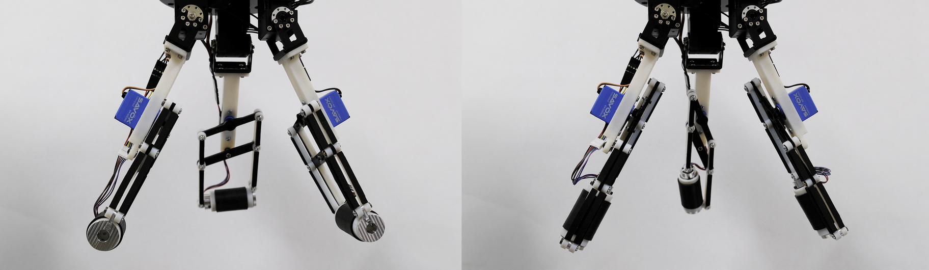

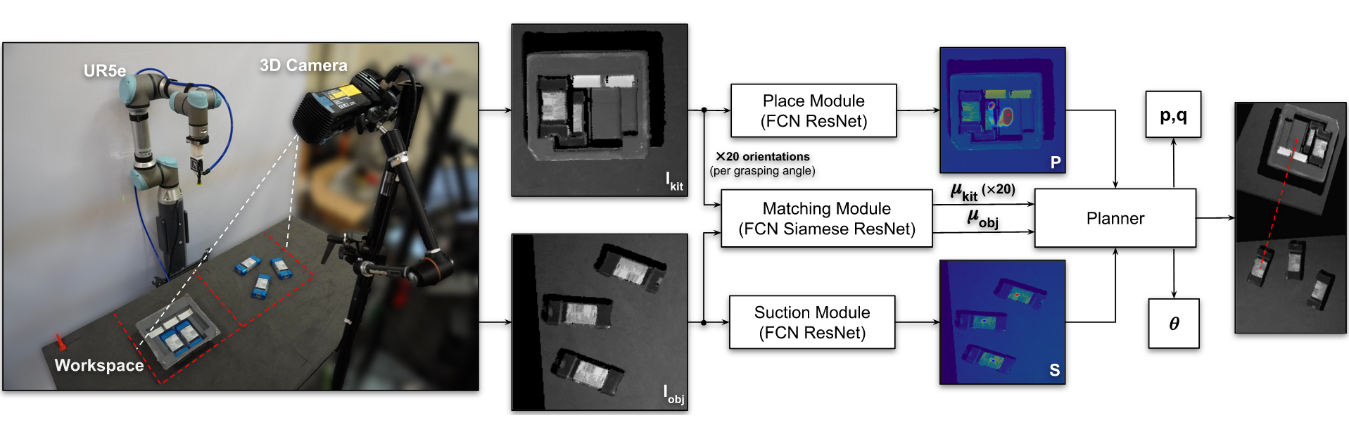
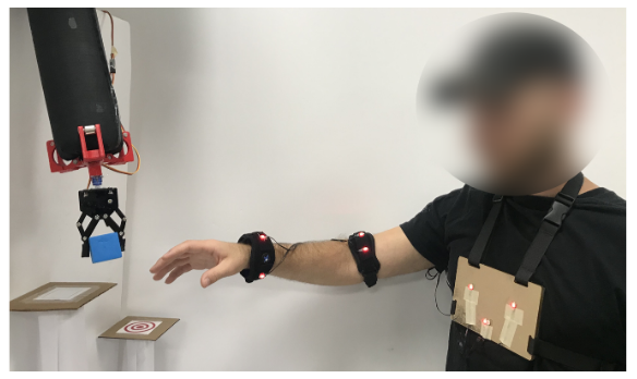
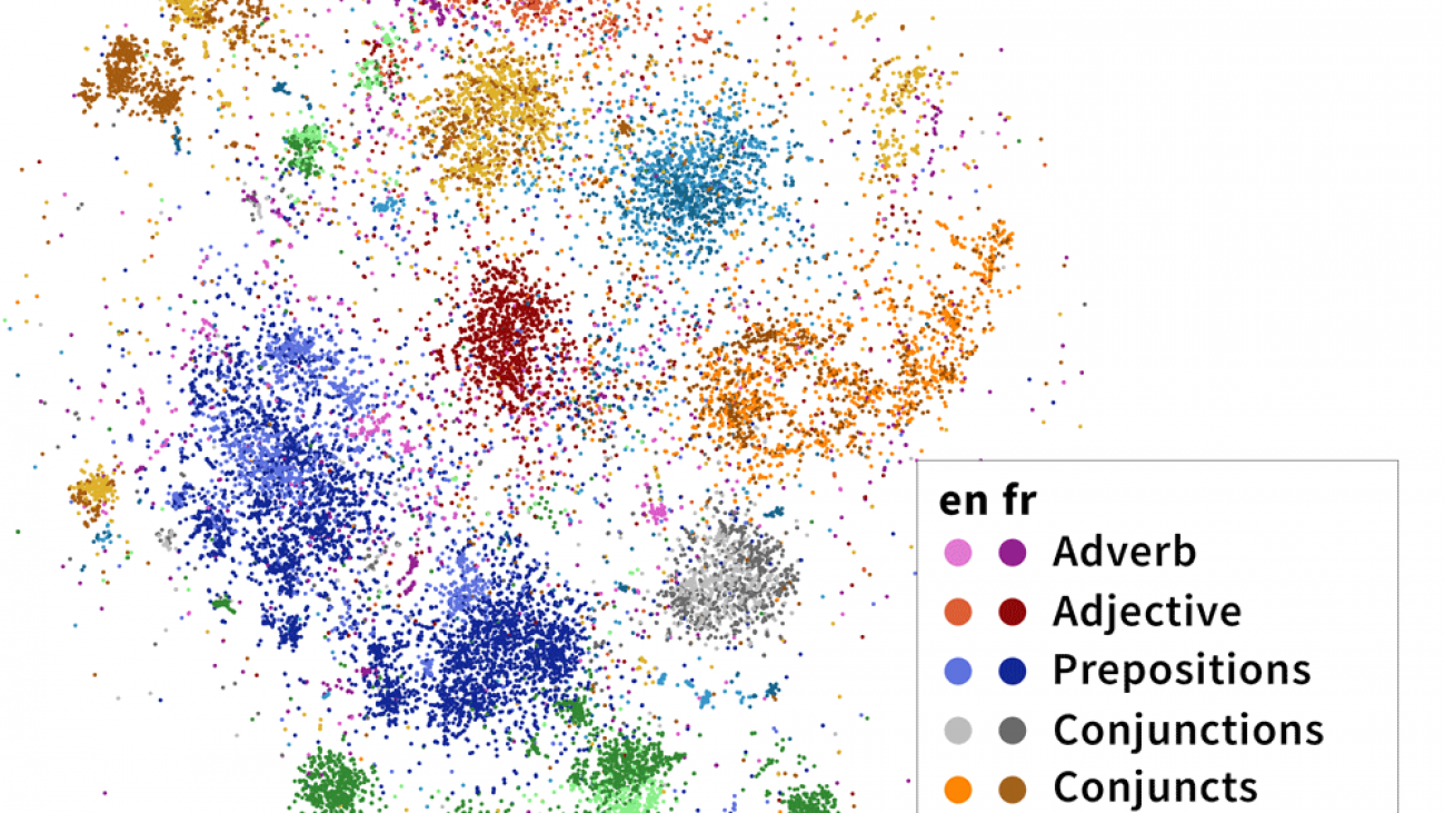
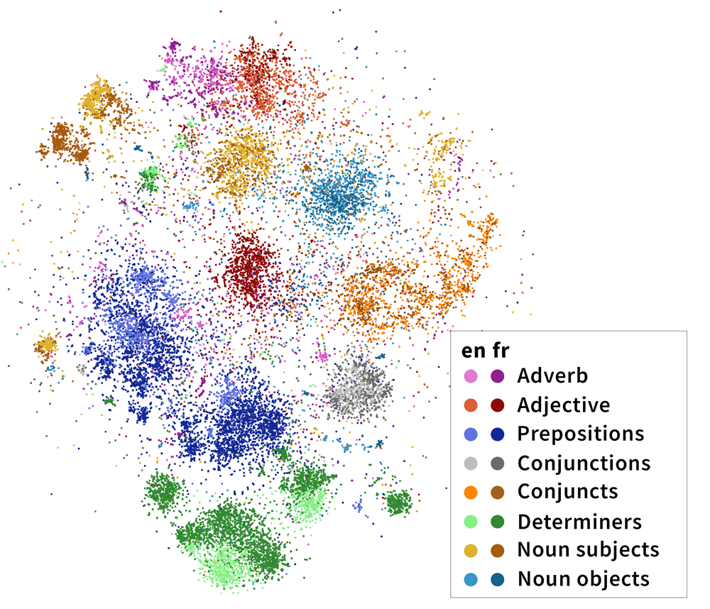

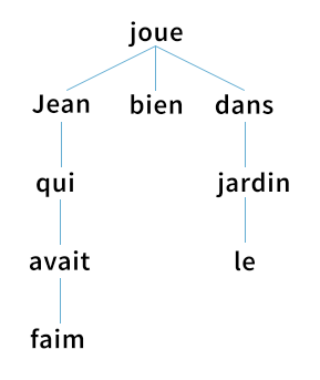
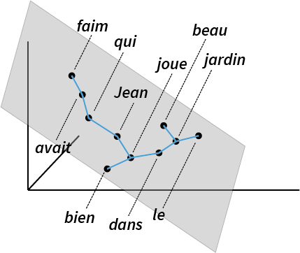
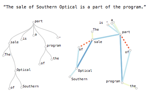
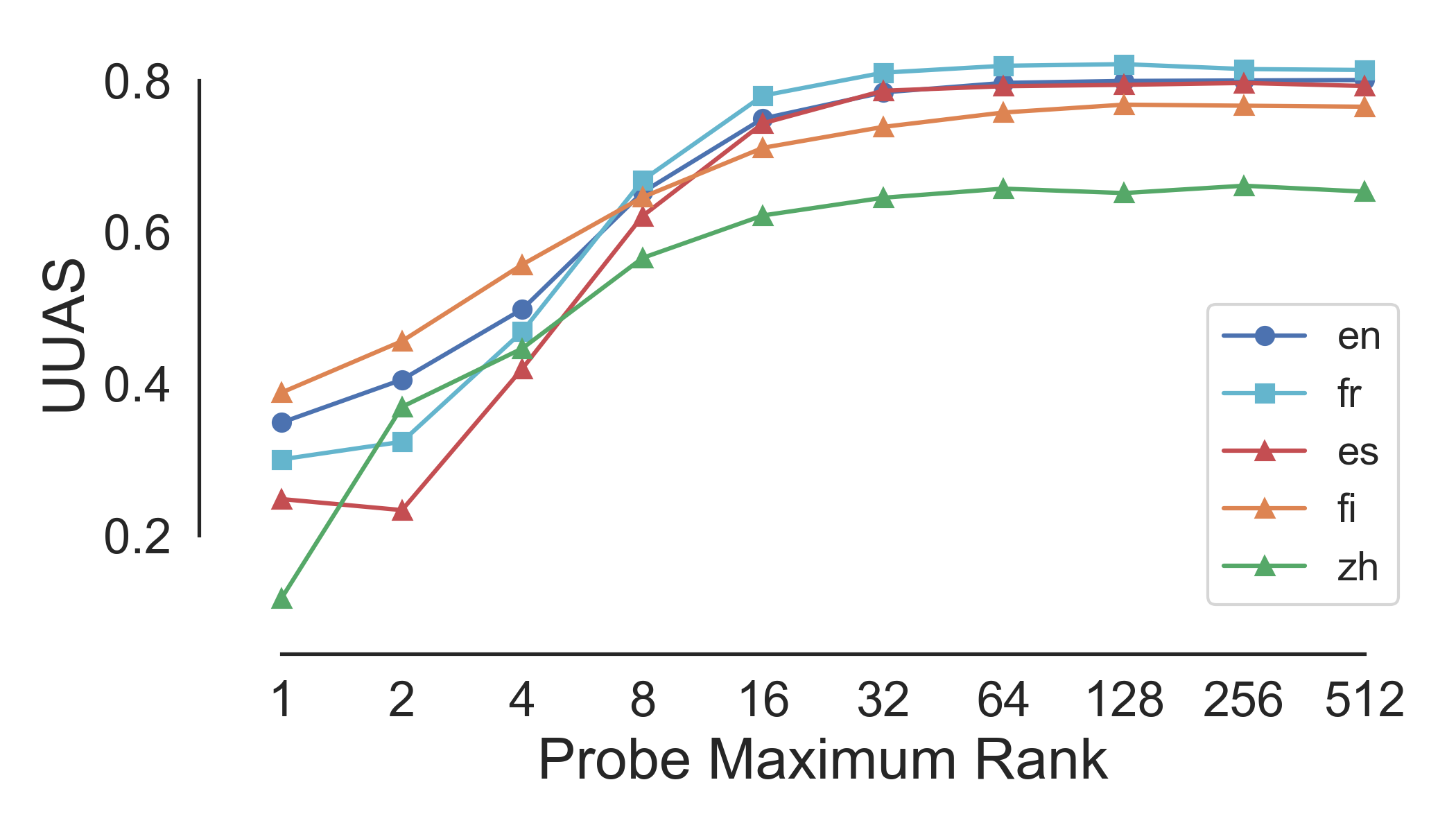
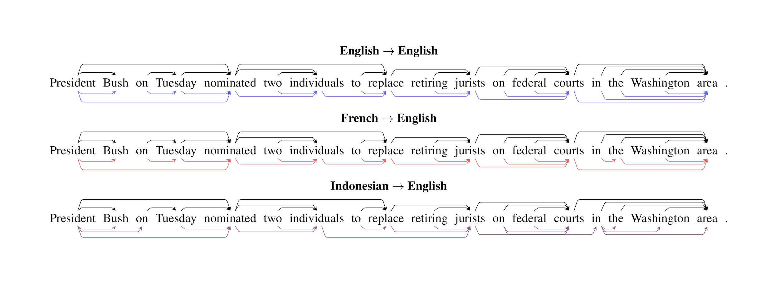
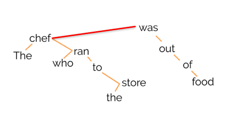
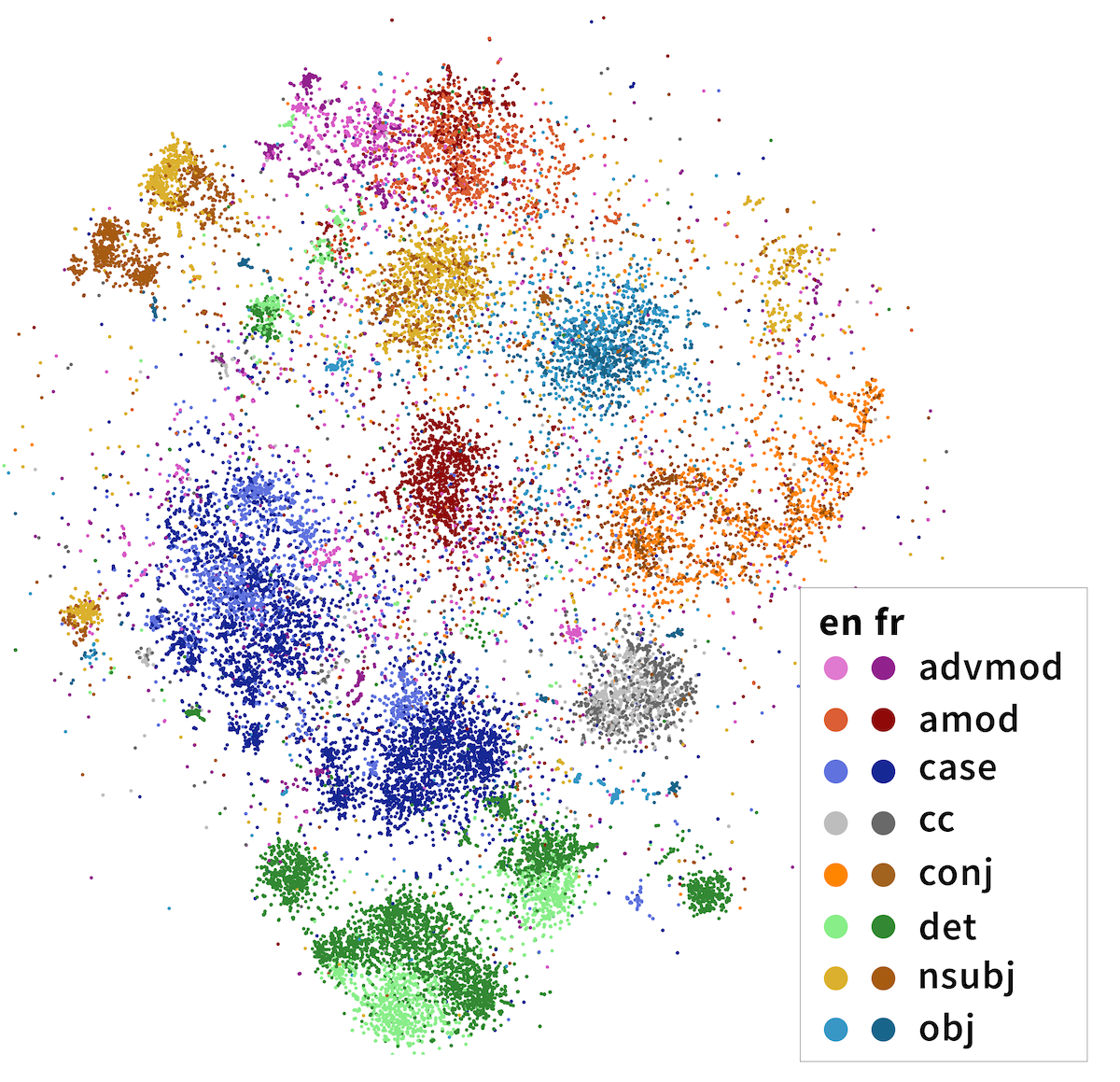
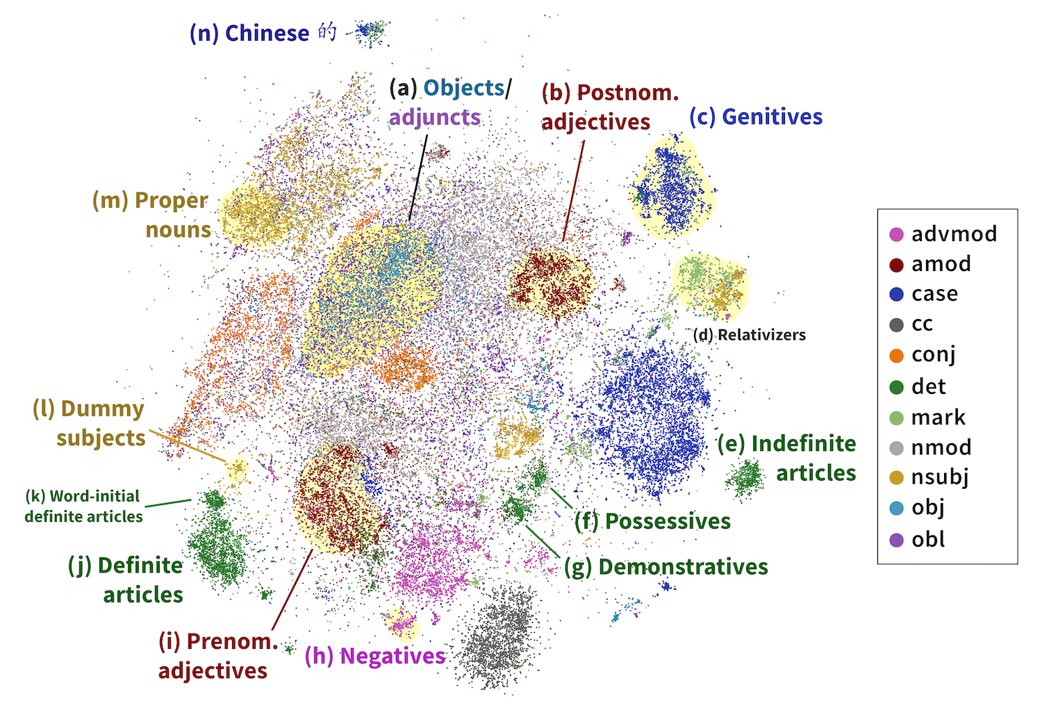
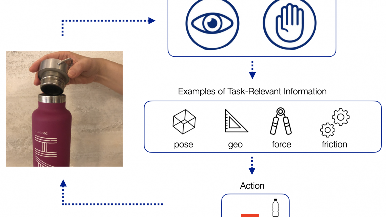
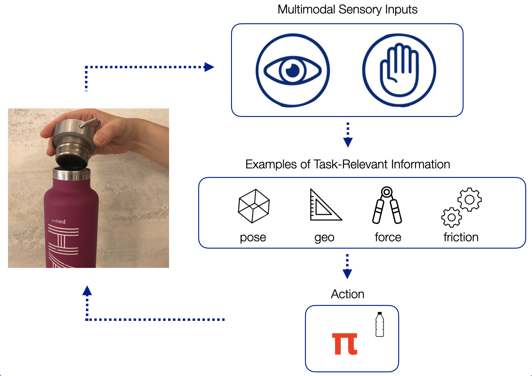
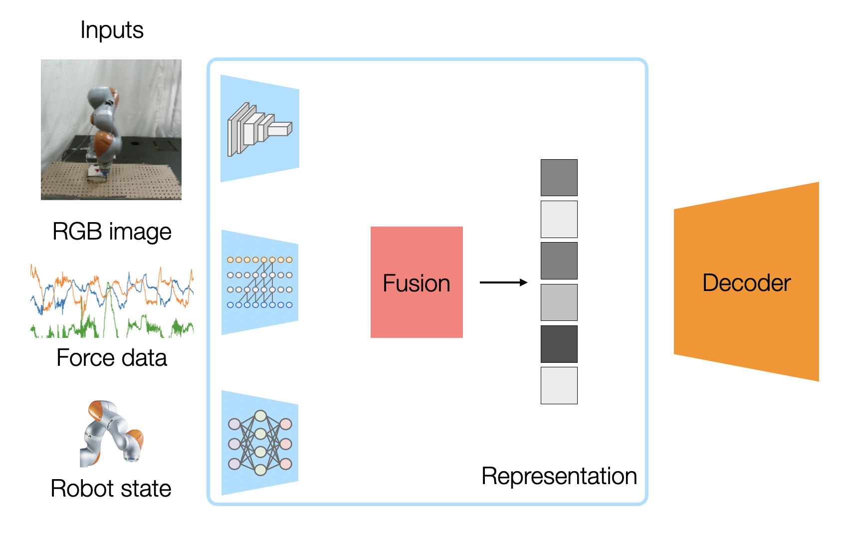
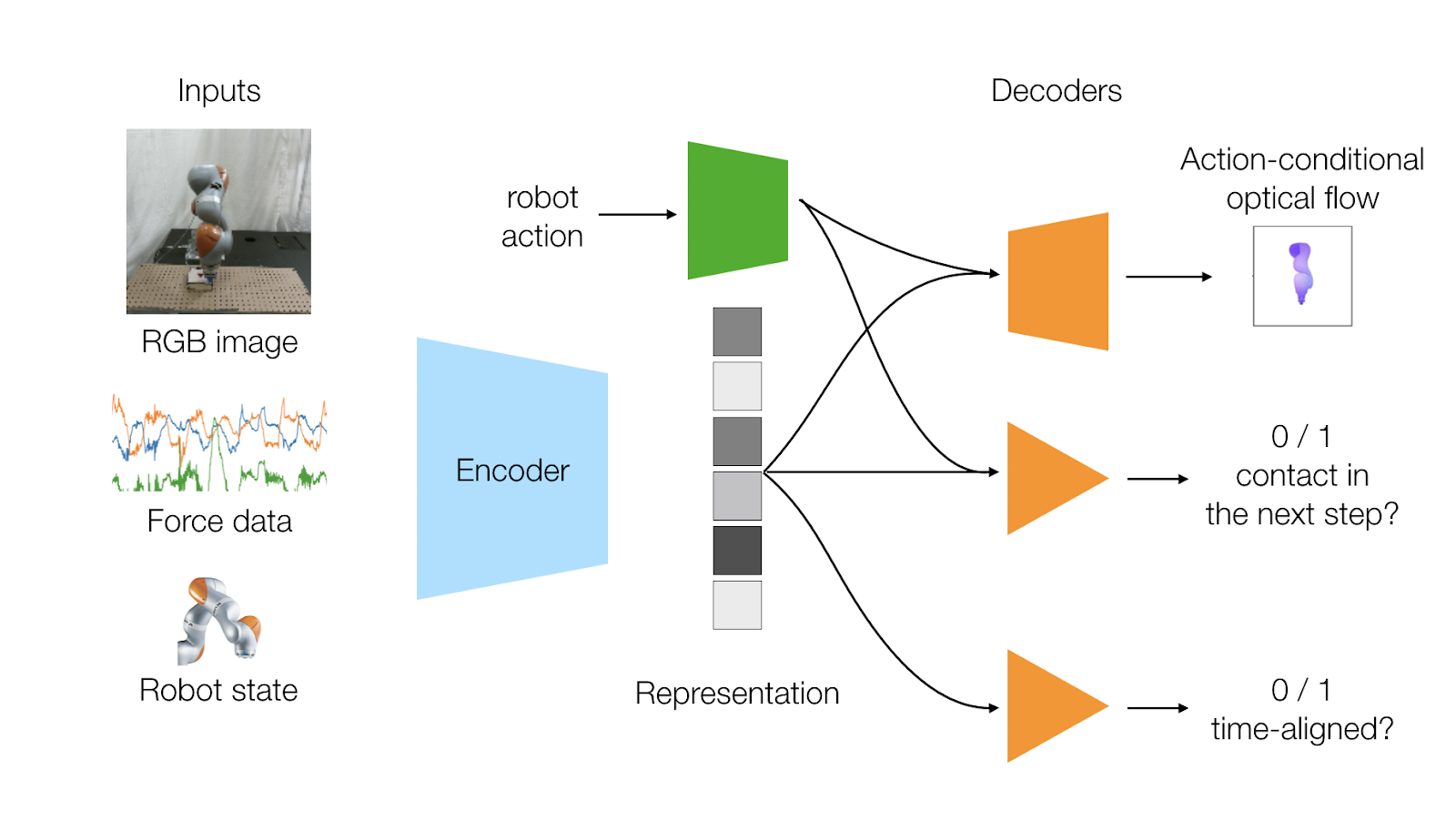

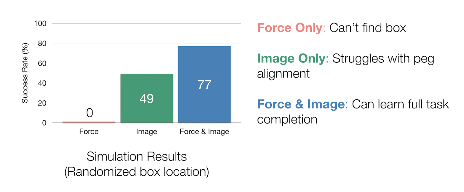
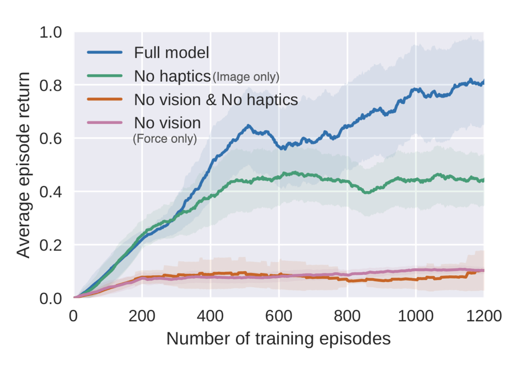
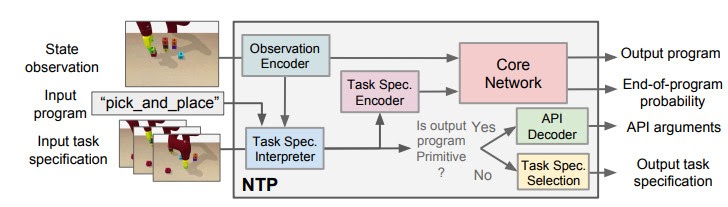
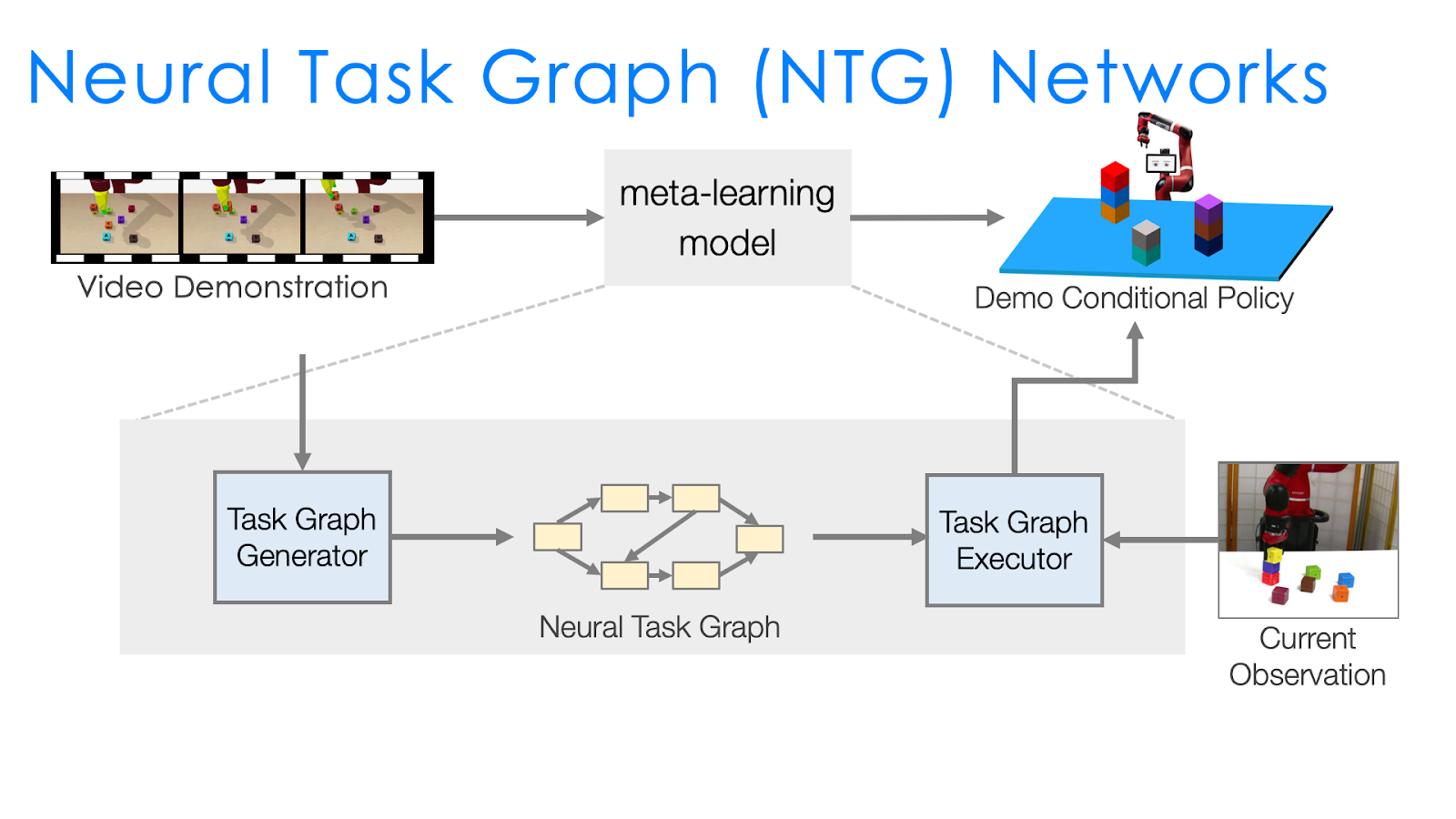
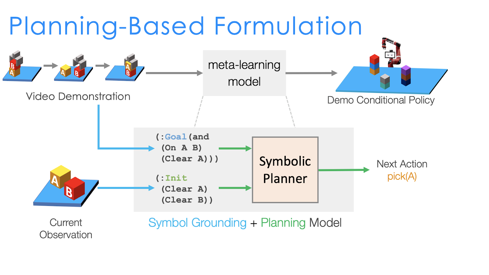
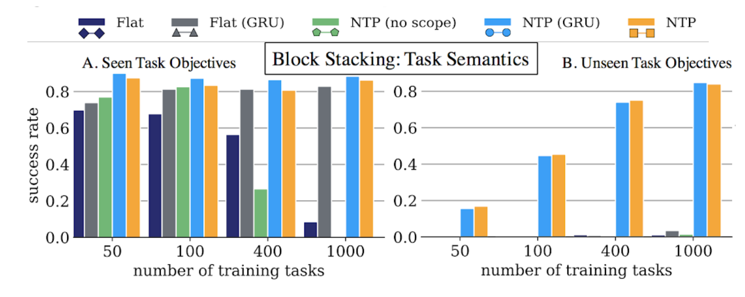
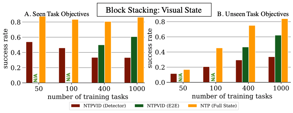
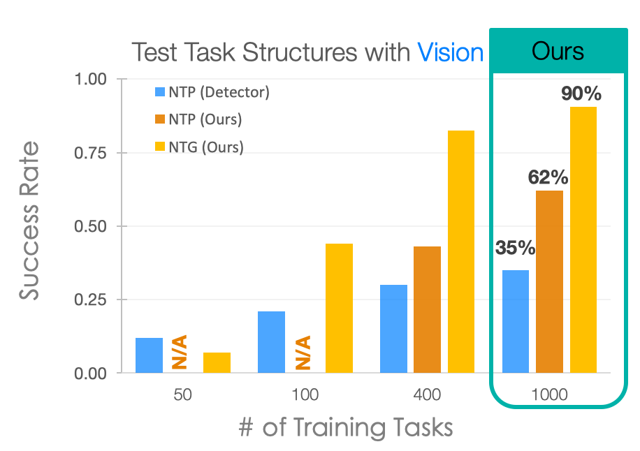
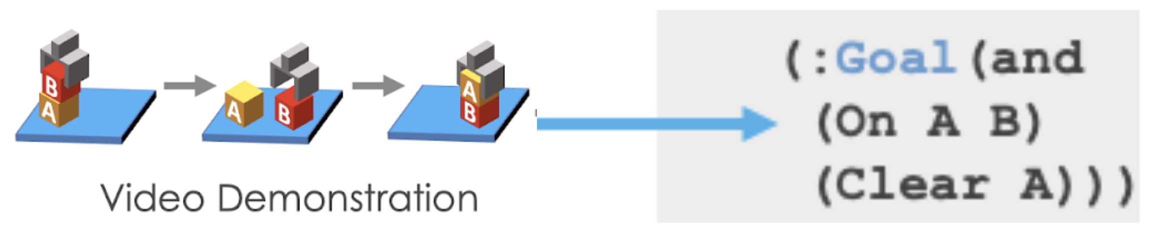
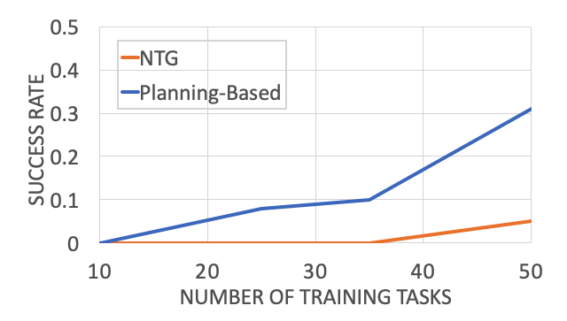


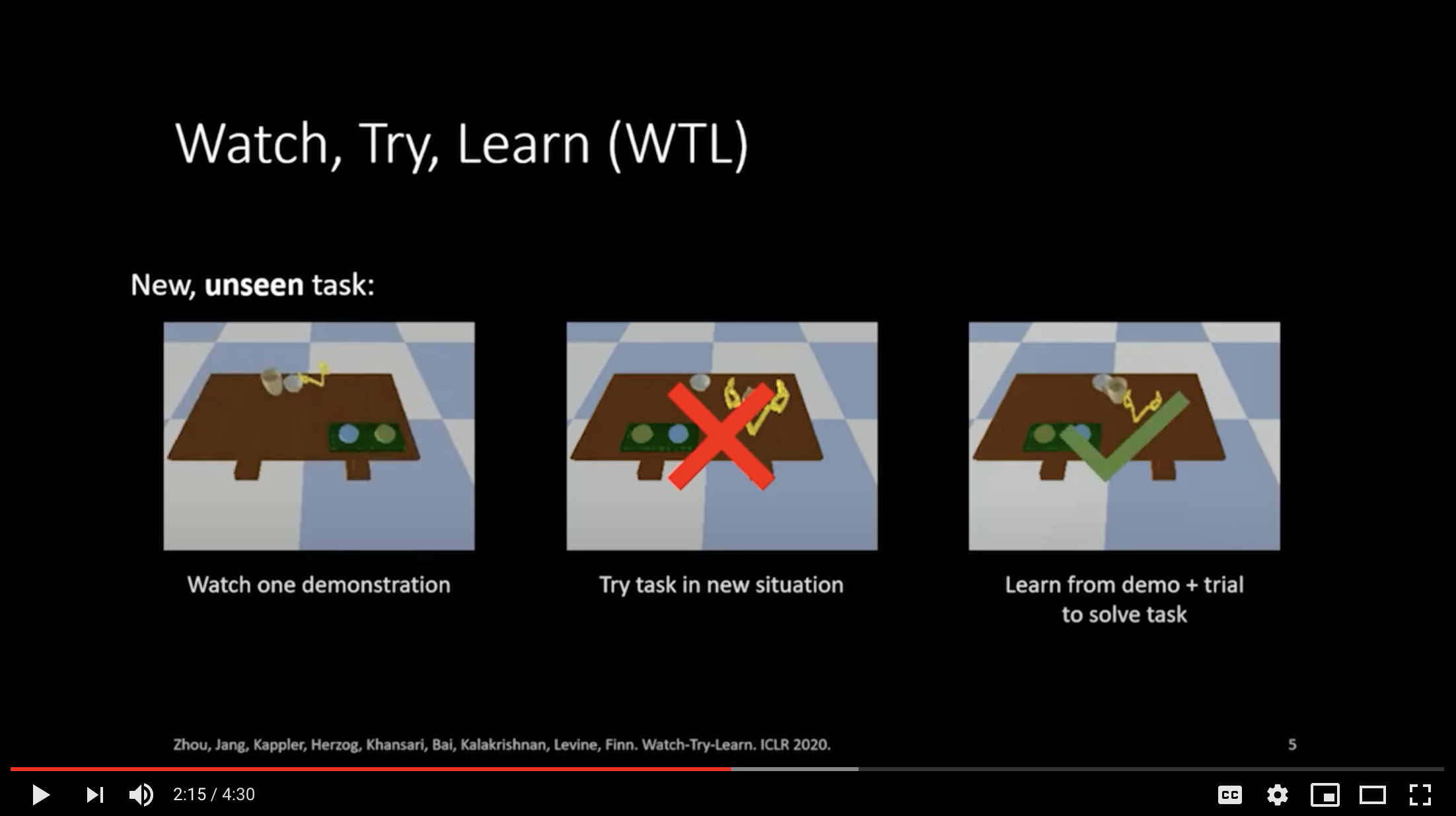


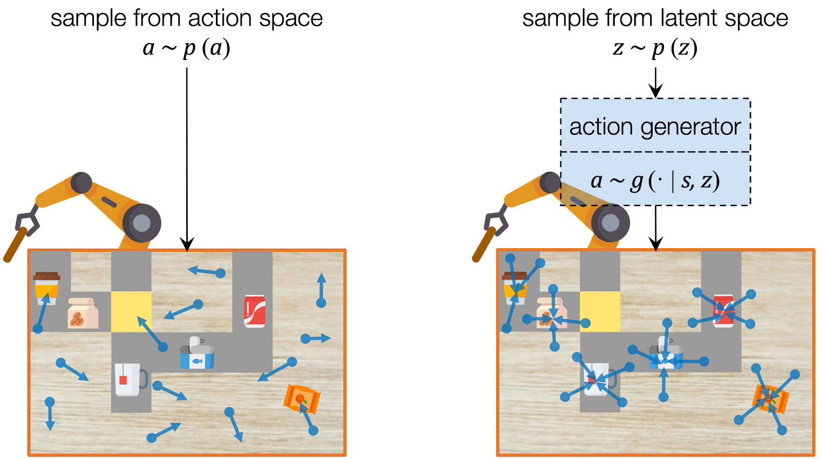
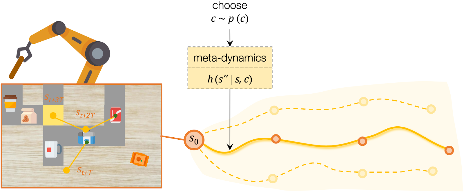
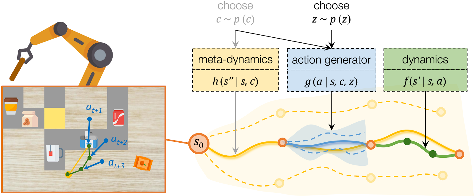
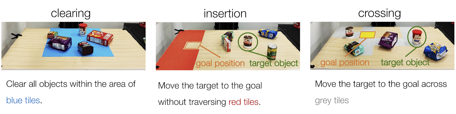
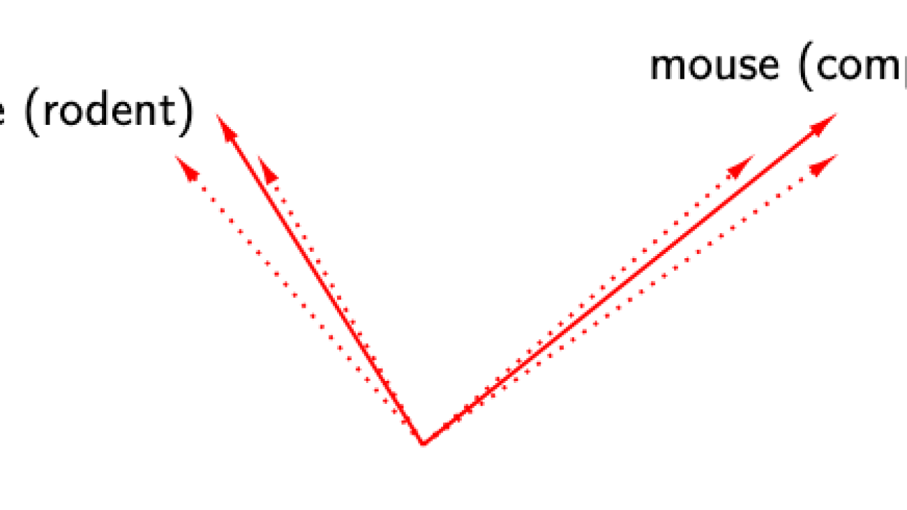
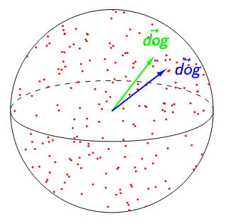 vs.
vs.