It takes a lot of data for robots to autonomously learn to perform simple manipulation tasks as as grasping and pushing. For example, prior work12 has leveraged Deep Reinforcement Learning to train robots to grasp and stack various objects. These tasks are usually short and relatively simple – for example, picking up a plastic bottle in a tray. However, because reinforcement learning relies on gaining experiences through trial-and-error, hundreds of robot hours were required for the robot to learn to picking up objects reliably.
It takes 100s of hours for robots to autonomously learn to perform manipulation tasks- even for grasping, or stacking, which are short-horizon tasks.
On the other hand, imitation learning can learn robot control policies directly from expert demonstrations without trial-and-error and thus require far less data than reinforcement learning. In prior work, a handful of human demonstrations have been used to train a robot to perform different skills such as pushing an object to a target location from only image input 3.
Imitation Learning has been used to directly learn short-horizon skills from 100-300 demonstrations.
However, because the control policies are only trained with a fixed set of task demonstrations, it is difficult for the policies to generalize outside of the training data. In this work, we present a method for learning to solve new tasks by piecing together parts of training tasks that the robot has already seen in the demonstration data.
A Motivating Example
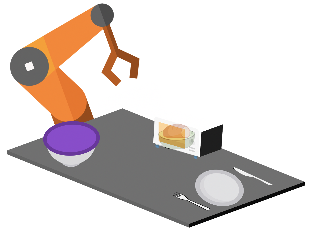
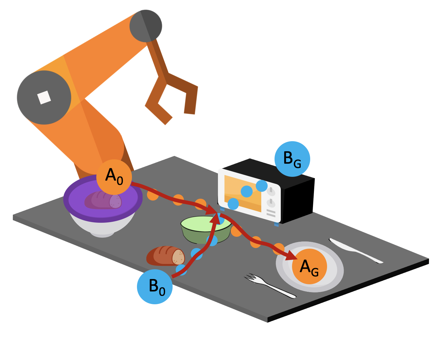
Consider the setup shown below. In the first task, the bread starts in the container, and the robot needs to remove the purple lid, retrieve the bread, put it into this green bowl, and then serve it on a plate.
In the first task, the robot needs to retrieve the bread from the covered container and serve it on a plate.
In the second task, the bread starts on the table, and it needs to be placed in the green bowl and then put into the oven for baking.
In the second task, the robot needs to pick the bread off the table and place it into the oven for baking.
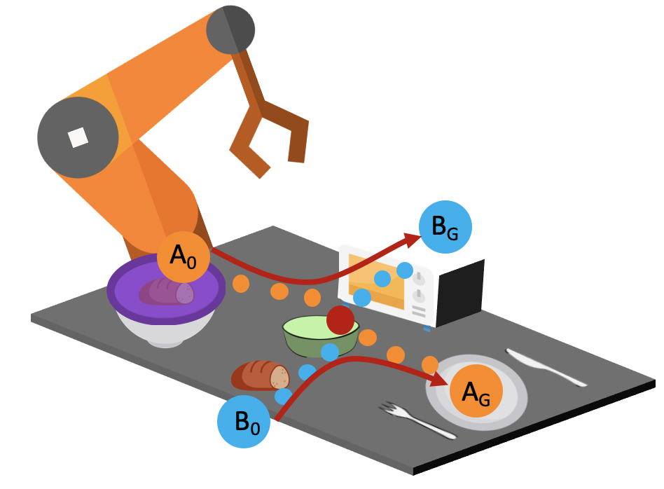
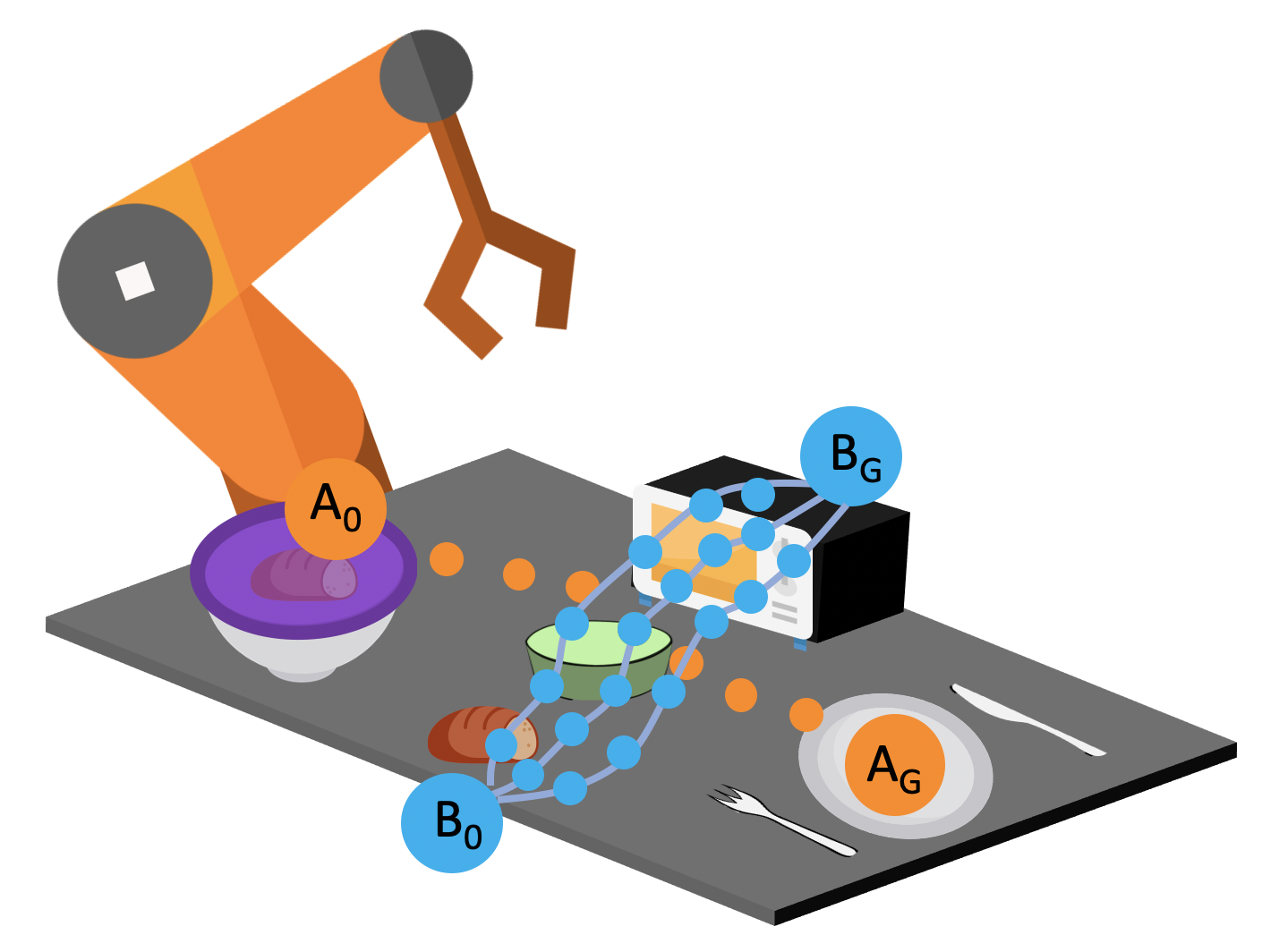
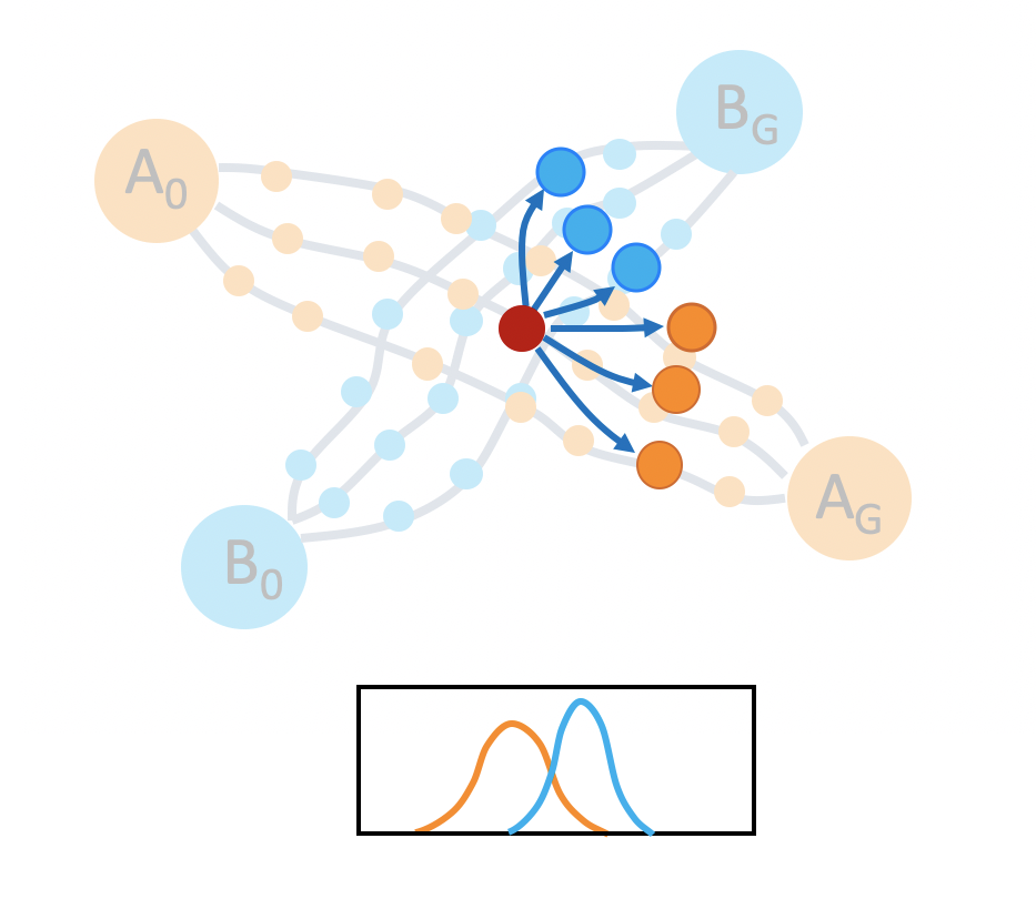
We provide the robot with demonstrations of both tasks. Note that both tasks require the robot to place the bread into this green bowl! In other words, these task trajectories intersect in the state space! The robot should be able to generalize to new start and goal pairs by choosing different paths at the intersection, as shown in the picture. For example, the robot could retrieve the bread from the container and place the bread into the oven, instead of placing it on the plate.
The task demonstrations for both tasks will intersect in the state space since both tasks require the robot to place the bread into the green bowl. By leveraging this task intersection and composing pieces of different demonstrations together, the robot will be able to generalize to new start and goal pairs.
In summary, our key insights are:
Multi-task domains often contain task intersections.
It should be possible for a policy to generate new task trajectories by composing training tasks via the intersections.
Generalization Through Imitation
In this work, we introduce Generalization Through Imitation (GTI), a two-stage algorithm for enabling robots to generalize to new start and goal pairs through compositional imitation.
Stage 1: Train policies to generate diverse (potentially new) rollouts from human demonstrations.
Stage 2: Use these rollouts to train goal-directed policies to achieve targeted new behaviors by self-imitation.
Generating Diverse Rollouts from Human Demonstrations
In Stage 1, we would like to train policies that are able to both reproduce the task trajectories in the data and also generate new task trajectories consisting of unseen start and goal pairs. This can be challenging – we need to encourage our trained policy to understand how to stop following one trajectory from the dataset and start following a different one in order to end up in a different goal state.
Here, we list two core technical challenges.
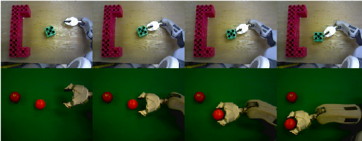
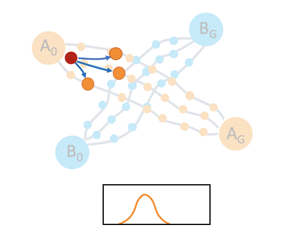
Mode Collapse. If we naively train imitation learning policies on the demonstration data of the two tasks, the policy tends to only go to a particular goal regardless of the initial states, as indicated by the red arrows in the picture below.
Spatio-temporal Variation There is a large amount of spatio-temporal variation from human demonstrations on a real robot that must be modeled and accounted for.
Generating diverse rollouts from a fixed set of human demonstrations is difficult due to the potential for mode collapse (left) and because the policy must also model spatio-temporal variations in the data (right).
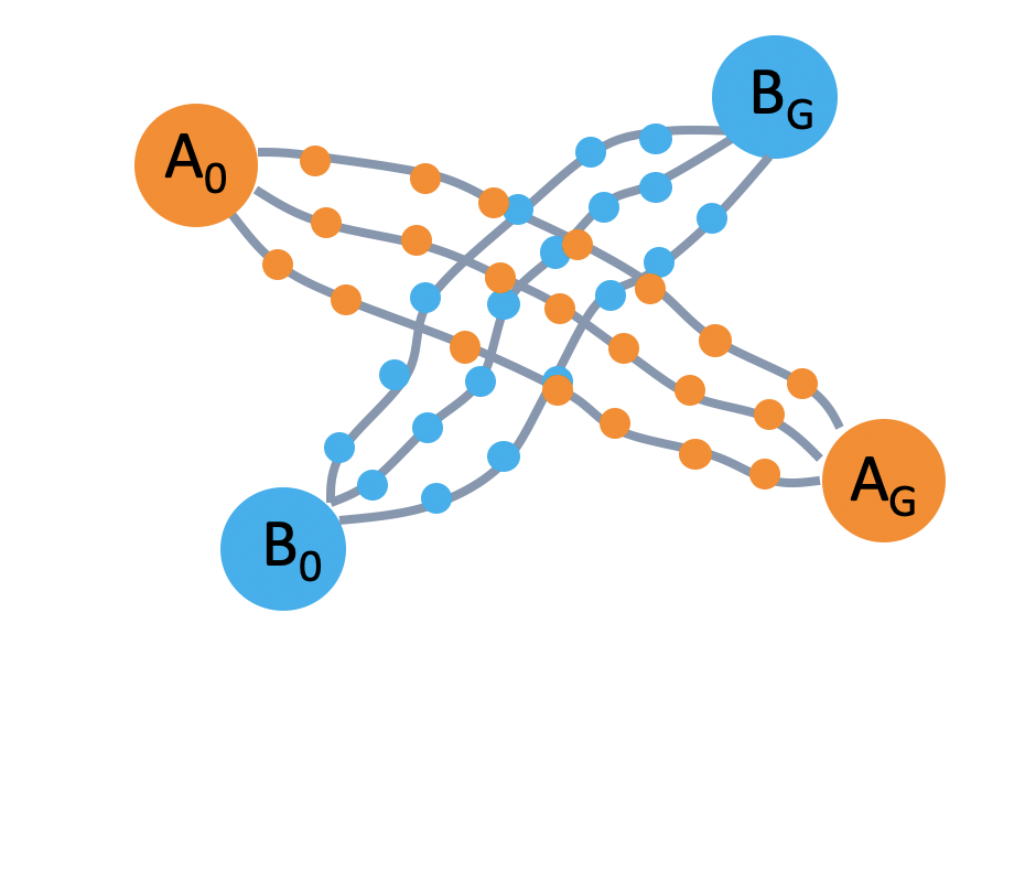
In order to get a better idea of how to encourage a policy to generate diverse rollouts, let’s take a closer look at the task space. The left image in the figure below shows the set of demonstrations. Consider a state near the beginning of a demonstration, as shown in the middle image. If we start in this state, and try to set a goal for our policy to achieve, according to the demonstration data, the goals can be modeled by a gaussian distribution. However, if we start at the intersection, the goal could spread across two tasks. It would be better for us to model the goal distributions with a multi-modal gaussian.
Task intersections are better modeled with mixtures of gaussians in order to capture the different possible future states.
Based on this observation, we design a hierarchical policy learning algorithm, where the high-level policy captures distribution of future observations in a multimodal latent space. The low-level policy conditions on the latent goal to fully explore the space of demonstrations.
GTI Algorithm Details
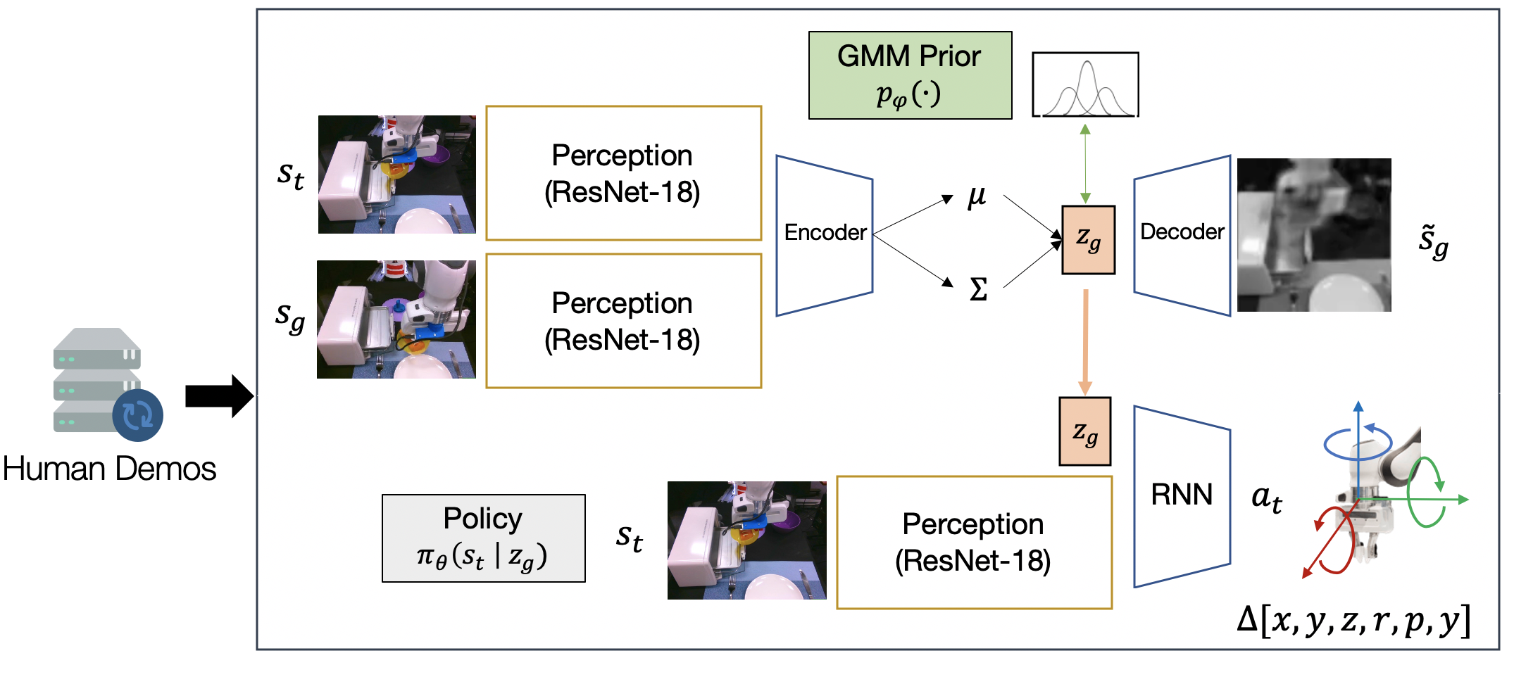
Let’s take a closer look at the learning architecture for our Stage 1 policy, shown below. The high-level planner is a conditional variational autoencoder4, that attempts to learn the distribution of future image observations conditioned on current image observations. The encoder encodes both a current and future observation into a latent space. The decoder attempts to reconstruct the future observation from the latent. The latent space is regularized with a learned Gaussian mixture model prior. This prior encourages the model to a latent multimodal distribution of future observations. We can think of this latent space as modeling short-horizon subgoals. We train our low-level controller to imitate actions in the dataset that lead to particular subgoals.
The diagram above depicts the Stage 1 training architecture.
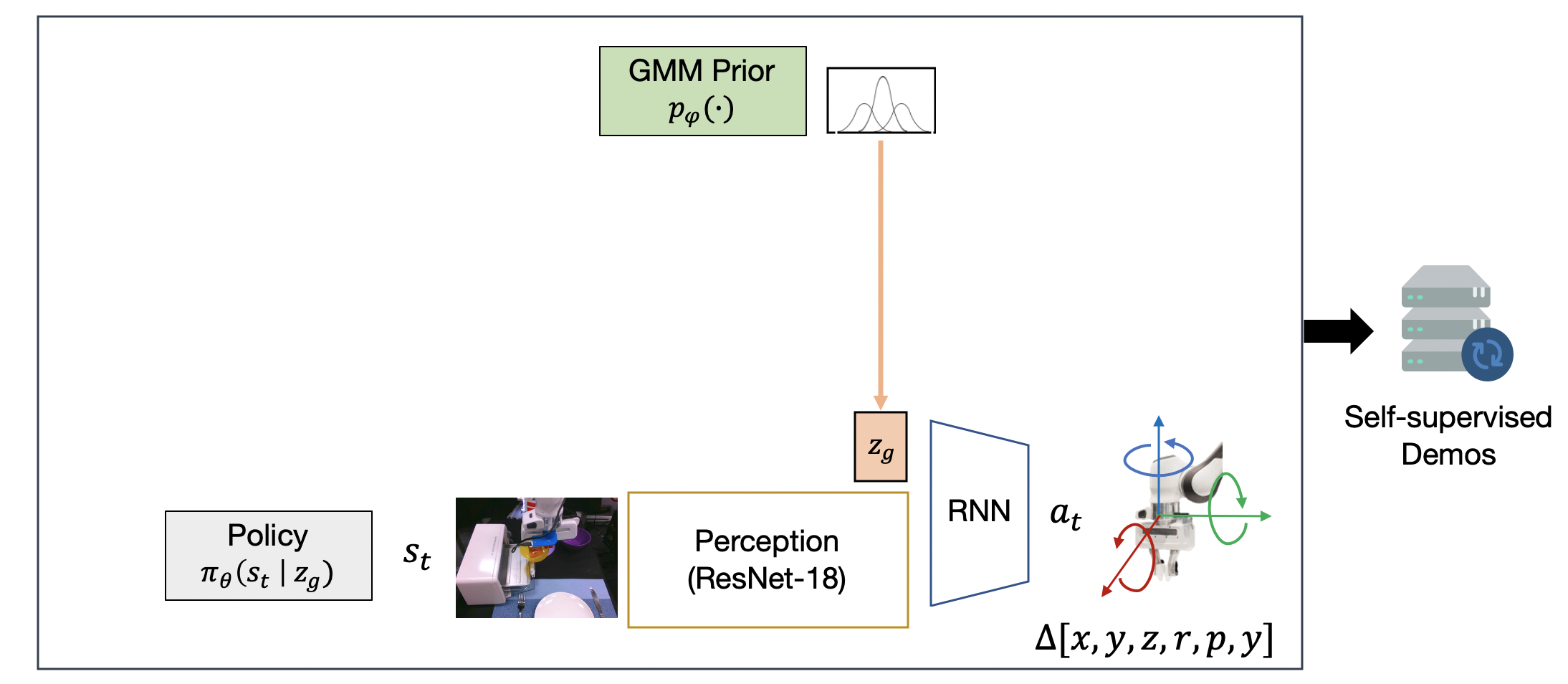
Next, we use the Stage 1 policy to collect a handful of self-generated diverse rollouts, shown below. Every 10 timesteps, we sample a new latent subgoal from the GMM prior, and use it to condition the low-level policy. The diversity captured in the GMM prior ensures that the Stage 1 policy will exhibit different behaviors at trajectory intersections, resulting in novel trajectories with unseen start and goal pairs.
The Stage 1 trained policy is used to generate a self-supervised dataset that covers the space of start and goal states by composing seen behaviors together.
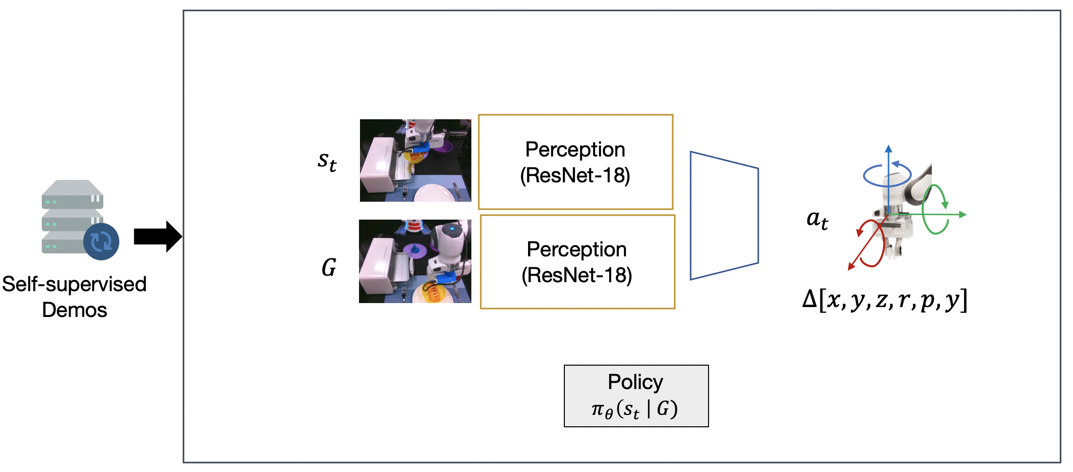
Finally, the self-generated dataset is used to train a new, goal-directed policy that can perform intentional behaviors from these undirected rollouts.
Stage 2 policy learning is just goal-conditioned behavioral cloning from the Stage 1 dataset, where the goals are final image observations from the trajectories collected in Stage 1.
Real Robot Experiments
Data Collection
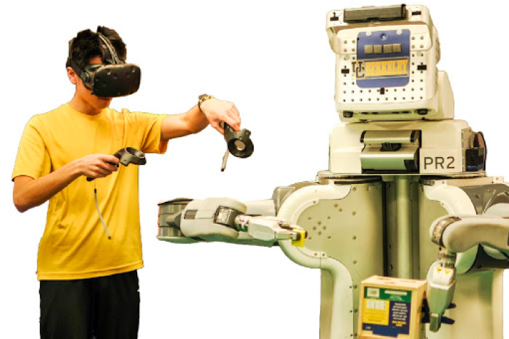
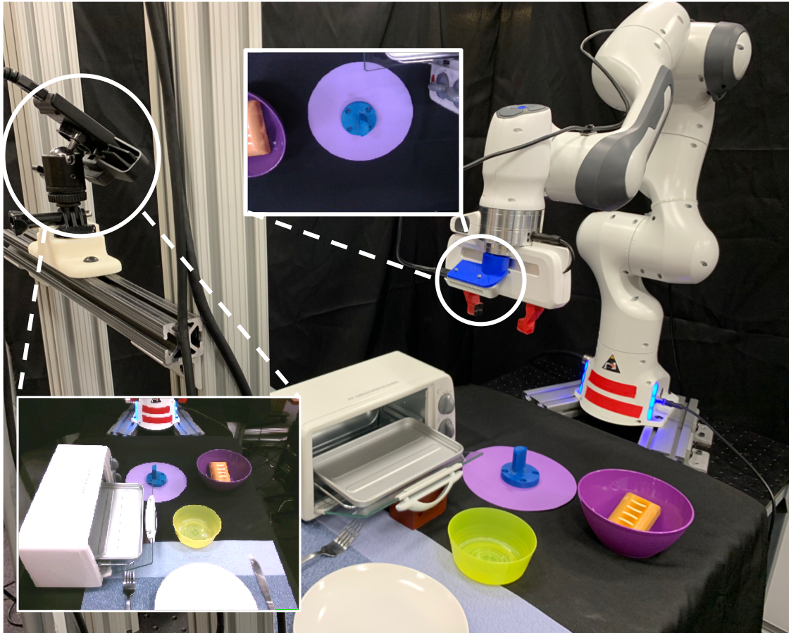
This is our hardware setup. We used a Franka robotic arm and two cameras for data collection – a front view camera and a wrist-mounted camera.
Hardware setup used in our work.
We used the RoboTurk phone teleoperation interface56 to collect human demonstrations. We collect only 50 demonstrations for each of the two tasks. The data collection took less than an hour.
We collected demonstrations using the RoboTurk phone teleoperation interface.
Results
Below, we show the final trained Stage 2 model. We ask the robot to start from the initial state of one task, bread-in-container, and reach the goal of the other task, which is to put the bread in the oven. The goal is specified by providing an image observation that shows the bread in the oven. We emphasize that the policy is performing closed-loop visuomotor control at 20hz purely from image observations. Note that this task requires accurate contact-rich manipulations, and is long-horizon. With only visual information, our method can perform intricate tasks such as grasping, pushing the oven tray into the oven, or manipulating a constrained mechanism like closing door of the oven.
GTI is able to produce a goal-conditioned policy that solves both tasks seen in the demonstrations and tasks that were not seen.
Our Stage 1 policy can recover all start and goal combinations, including both behavior seen in training and new unseen behaviors.
The GTI Stage 1 policy can imitate the demonstrations to solve the tasks seen in the demonstrations.
The GTI Stage 1 policy can compose different parts of the demonstrations together to produce novel behavior and solve unseen tasks as well.
Finally, we show that our method is robust towards unexpected situations. In the case below (left), the policy is stuck because of conflicting supervisions. Sampling latent goals allows the policy to get unstuck and complete the task successfully. Our policy is also very reactive and can quickly recover from errors. In the case below (right), the policy failed to grasp the bread twice, and finally succeeded the third time. It also made two attempts to get a good grasp of the bowl, and complete the task successfully
Robustness results. The policy is able to deal with conflicting supervision and get unstuck by sampling latent goals (left). The policy is reactive and can quickly recover from errors (right).
Summary
Imitation learning is an effective and safe technique to train robot policies in the real world because it does not depend on an expensive random exploration process. However, due to the lack of exploration, learning policies that generalize beyond the demonstrated behaviors is still an open challenge.
Our key insight is that multi-task domains often present a latent structure, where demonstrated trajectories for different tasks intersect at common regions of the state space.
We present Generalization Through Imitation (GTI), a two-stage offline imitation learning algorithm that exploits this intersecting structure to train goal-directed policies that generalize to unseen start and goal state combinations.
We validate GTI on a real robot kitchen domain and showcase the capacity of trained policies to solve both seen and unseen task configurations.
Quillen, D., Jang, E., Nachum, O., Finn, C., Ibarz, J., & Levine, S. (2018, May). Deep reinforcement learning for vision-based robotic grasping: A simulated comparative evaluation of off-policy methods. In 2018 IEEE International Conference on Robotics and Automation (ICRA) (pp. 6284-6291). IEEE. ↩
Cabi, S., Colmenarejo, S. G., Novikov, A., Konyushkova, K., Reed, S., Jeong, R., … & Sushkov, O. (2019). A Framework for Data-Driven Robotics. arXiv preprint arXiv:1909.12200. ↩
Zhang, T., McCarthy, Z., Jow, O., Lee, D., Chen, X., Goldberg, K., & Abbeel, P. (2018, May). Deep imitation learning for complex manipulation tasks from virtual reality teleoperation. In 2018 IEEE International Conference on Robotics and Automation (ICRA) (pp. 1-8). IEEE. ↩
Kingma, D. P., & Welling, M. (2013). Auto-encoding variational bayes. arXiv preprint arXiv:1312.6114. ↩
Mandlekar, A., Zhu, Y., Garg, A., Booher, J., Spero, M., Tung, A., … & Savarese, S. (2018). Roboturk: A crowdsourcing platform for robotic skill learning through imitation. arXiv preprint arXiv:1811.02790. ↩
Mandlekar, A., Booher, J., Spero, M., Tung, A., Gupta, A., Zhu, Y., … & Fei-Fei, L. (2019). Scaling Robot Supervision to Hundreds of Hours with RoboTurk: Robotic Manipulation Dataset through Human Reasoning and Dexterity. arXiv preprint arXiv:1911.04052. ↩
When editing or revising we often write in a non-linear manner.
Writing an email
An existing system might suggest something like “great to me” because it only considers the preceding text but not the subsequent text.
A better suggestion in this case would be something like “good with one exception” since the writer is not completely satisfied and suggesting a further revision.
Writing a novel
When you don’t have a concrete idea on how to connect two scenes, the system can suggest a way to connect the fragmented ideas.
Task
Fill in the blanks?
Consider the following sentence with blanks:
She ate ____ for ____
To fill in the blanks, one needs to consider both preceding and subsequent text (in this case, “She ate” and “for”). There can be many reasonable ways to fill in the blanks:
She ate leftover pasta for lunch
She ate chocolate ice cream for dessert
She ate toast for breakfast before leaving for school
She ate rather quickly for she was in a hurry that evening
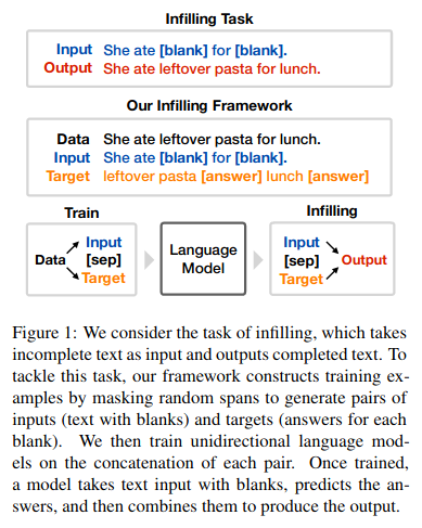
The task of filling in the blanks is known as text infilling in the field of Natural Language Processing (NLP). It is the task of predicting blanks (or missing spans) of text at any position in text.
The general definition of text infilling considers text with an arbitrary number of blanks where each blank can represent one of more missing words.
Language models?
Language modeling is a special case of text infilling where only the preceding text is present and there is only one blank at the end.
She ate leftover pasta for ____
In recent few years, a number of large-scale language models are introduced and shown to achieve human-like performance. These models are often pre-trained on massive amount of unlabeled data, requiring huge amount of computation and resource.
Our goal is to take these existing language models and make them perform the more general task of filling in the blanks.
Approach
How can we make a language model fill in the blanks?
Our approach is infilling by language modeling. With this approach, one can simply (1) download an existing pre-trained language model and (2) enable it to fill in any number and length of blanks in text by fine-tuning it on artificially generated examples.
Main advantages of our framework are as follows:
Conceptual simplicity: Minimal change to standard language model training
Model-agnostic framework: Leverage massively pre-trained language models
Now, let’s see what happens at training and test time!
Training time
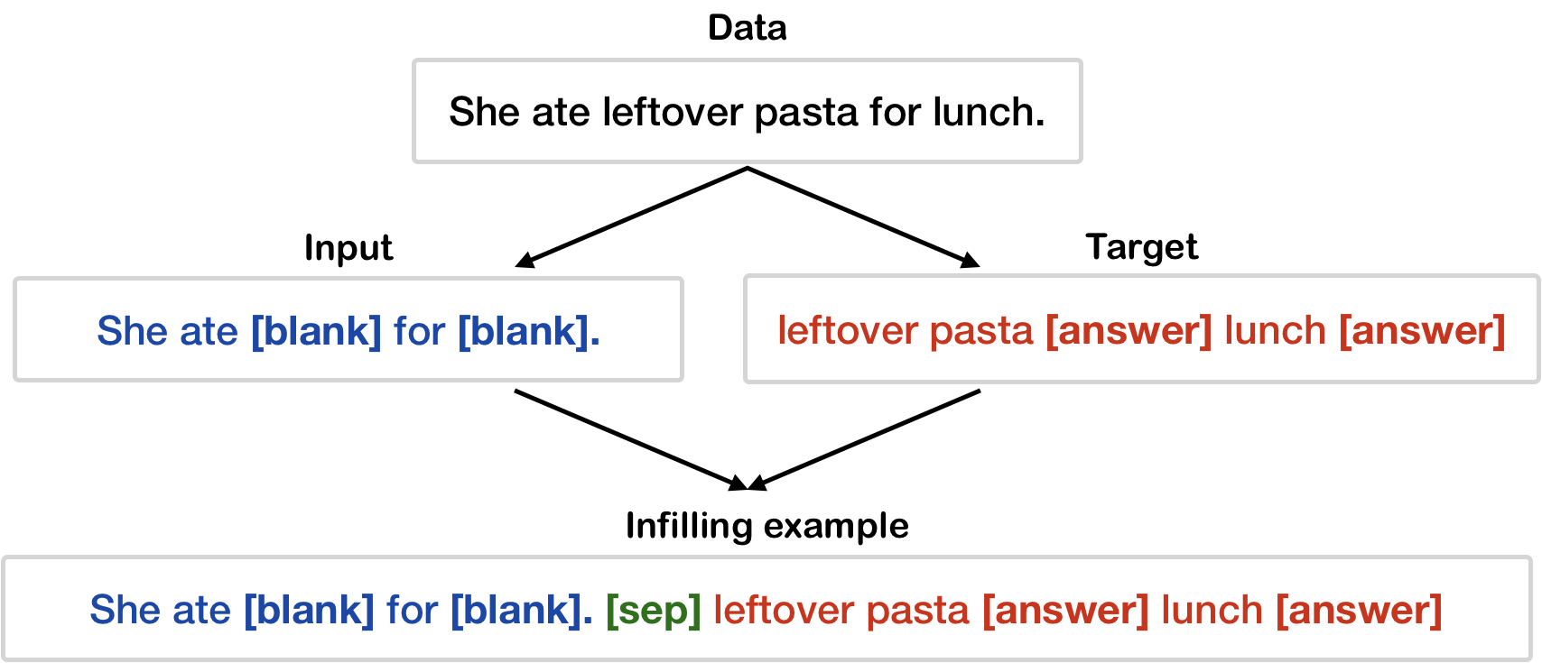
1. Manufacture infilling examples
Suppose we have plain text as our data:
Data: She ate leftover pasta for lunch.
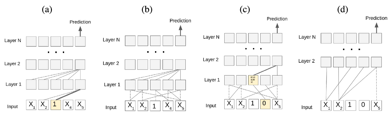
To produce an infilling example for given data, first generate input by randomly replacing some tokens in the data with [blank] tokens.
Input: She ate [blank] for [blank].
Then, generate a target by concatenating the replaced tokens, separated by the [answer] token.
Target: leftover pasta [answer] lunch [answer]
Finally, construct the complete infilling example by concatenating input, a special separator token [sep], and target.
Infilling example: She ate [blank] for [blank]. [sep] leftover pasta [answer] lunch [answer]
Looking for a script to automate this step? It is available here!
Now, let’s fine-tune the model on the infilling examples using standard language model training methodology.
Test time
Once trained, we can use the language model to infill at test time.
As input, the model takes incomplete text with [blank] and generates a target.
Input: He drinks [blank] after [blank].
Target: water [answer] running [answer]
You can then construct the complete text by simply replacing [blank] tokens in the input with predicted answers in the target in a deterministic fashion.
Output: He drinks water after running.
Practical advantages
Our framework incurs almost no computational overhead compared to language modeling. This is particularly good when considering models like GPT-2 whose memory usage grows quadratically with sequence length.
Our framework requires minimal change to the vocabulary of existing language models. Specifically, you need three additional tokens: [blank], [answer], and [sep].
Our framework offers the ability to attend to the entire context on both sides of a blank with the simplicity of decoding from language models.
Evaluation
Turing test
The following is a short story consisting of five sentences. One of the sentences is swapped with a sentence generated by our model. Can you find it?
Q. Identify one of the five sentences generated by machine.
[1] Patty was excited about having her friends over.
[2] She had been working hard preparing the food.
[3] Patty knew her friends wanted pizza.
[4] All of her friends arrived and were seated at the table.
[5] Patty had a great time with her friends.
Q. Identify one of the five sentences generated by machine.
[1] Yesterday was Kelly’s first concert.
[2] She was nervous to get on stage.
[3] When she got on stage the band was amazing.
[4] Kelly was then happy.
[5] She couldn’t wait to do it again.
(Answers are at the end of the post.)
In our experiments, we sampled a short story from ROCstories (Mostafazadeh et al., 2016), randomly replaced one of the sentences with a [blank] token, and infilled with a sentence generated by a model. Then, we asked 100 people to identify which of the sentences in a story was machine-generated.
System
How many people were fooled?
Generated sentence
BERT (Devlin et al., 2019)
20%
favoritea “, Mary brightly said.
Self-Attention Model (Zhu et al., 2019)
29%
She wasn’t sure she had to go to the store.
Standard Language Model (Radford et al., 2019)
41%
She went to check the tv.
Infilling by Language Model (Ours)
45%
Patty knew her friends wanted pizza.
Human
78%
She also had the place looking spotless.
The results show that people have difficulty identifying sentences infilled by our model as machine-generated 45% of the time. Generated sentences in the table are the system outputs for sentence [3] in the first story of the Turing test.
More experiments and analysis can be found in our paper.
Try it out!
We have a demo where you can explore the infilling functionality for
multiple variable-length spans and different granularities (e.g. words, phrases, and sentences)
on the domains of short stories, scientific abstracts, and song lyrics!
You can check out our paper on arXiv and our source code on GitHub.
You can also find a short talk on this work here. If you have questions, please feel free to email us!
With autonomous systems becoming more capable, they are entering into safety-critical domains such as autonomous driving, aircraft collision avoidance, and healthcare. Ensuring the safe operations of these systems is a crucial step before they can be deployed and accepted by our society. Failure to perform the proper degree of safety validation can risk the loss of property or even human life.
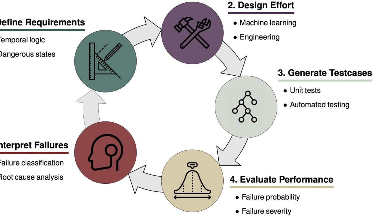
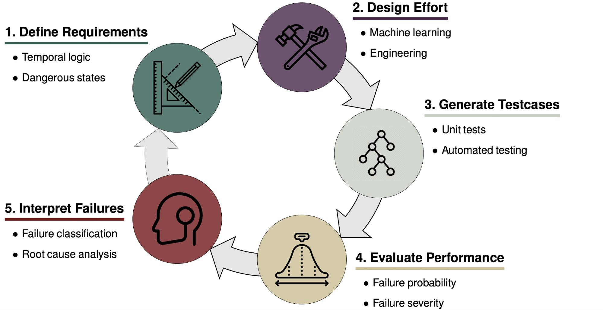
The autonomous system design cycle.
Safety can be incorporated at various stages of the development of an autonomous system. Consider the above model for the design cycle of such a system. A necessary component of safety is the definition of a complete set of realistic and safe requirements such as the Responsibility-Sensitive Safety model1 which encodes commonsense driving rules—such as don’t rear end anyone and right of way is given, not taken—into formal mathematical statements about what a vehicle is and is not allowed to do in a given driving scenario. Safety can also be incorporated directly into the design of the system through techniques such as safety-masked reinforcement learning (RL)2 where a driving agent learns how to drive under the constraint that it only takes actions that have a minimal likelihood of causing a collision. Compared to traditional reinforcement learning techniques which have no constraint on their exploratory actions, safety-masked RL results in a safer driving policy.
Once a prototype of a system is available, safety validation can be performed through testing, performance evaluation, and interpretation of the failure modes of the system. Testing can discover failures due to implementation bugs, missing requirements, and emergent behavior due to the complex interaction of subcomponents. For complex autonomous systems operating in physical environments, we can not guarantee safety in all situations, so performance evaluation techniques can determine if the system is acceptably safe. The failure examples generated from testing can then be used to understand flaws in the systems and help engineers to fix them in the next iteration. Even with safety embedded in the process of defining requirements and system design, safety validation is a critical part of ensuring safe autonomy.
There are multiple ways to go about safety validation. White-box approaches use knowledge of the design of the system to construct challenging scenarios and evaluate the behavior of the system. They are often interpretable and can give a high degree of confidence in a system, but can suffer from problems of scalability. Modern autonomous systems employ complex components such as deep neural networks for perception and decision making. Despite improvements to white-box approaches for small neural networks3, they don’t scale to the large networks used in practice. We can, however, trade formal guarantees for scalability by employing algorithms that treat the autonomous system as a black-box.
Safety validation algorithms for black-box autonomous systems have become the preferred tool for validation since they scale to complex systems and can rely on the latest advancements in machine learning to become more effective. In this blog post we cover the latest research in algorithms for the safety validation of black box autonomous systems. For a more in-depth description of the following algorithms (including pseudocode) see our recent survey paper A Survey of Algorithms for Black-Box Safety Validation.
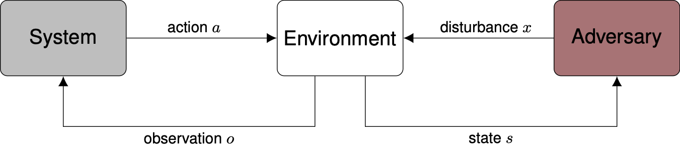
The problem formulation for the safety validation of black-box autonomous systems.
The setup for safety validation algorithms for black-box systems is shown above. We have a black-box system that is going to be tested, such as an autonomous vehicle driving policy or an aircraft collision avoidance system. We assume we have a simulated environment in which the system takes actions after making observations with its sensors, while an adversary perturbs the environment through disturbances in an effort to make the system fail. Disturbances could include sensor noise, the behavior of other agents in the environment, or environmental conditions such as weather. The adversary may have access to the state of the environment which, for example, may describe the positions and velocity of all the vehicles and pedestrians in a driving scenario. The systems we care about usually operate over time in a physical environment, in which case the adversary seeks to find the sequence of disturbances that leads to failure. Finding a disturbance trajectory that leads to failure, rather than just a single disturbance, makes the problem much more challenging. We may also have a model of the disturbances in the environment that describes which sequences of disturbances are most likely. The disturbance model can be constructed through expert knowledge or learned from real-world data. The exact goal of the adversary may be
Falsification: Find any disturbance trajectory that leads to a failure.
Most likely failure analysis: Find the most likely disturbance trajectory that leads to a failure (i.e. maximize ).
Estimation of the probability of failure: Determine how likely it is that any failure will occur based on knowledge of .
The adversary can use a variety of algorithms to generate disturbances. We will cover 4 categories: optimization, path-planning, reinforcement learning, and importance sampling.
Optimization
Optimization approaches search over the space of possible disturbance trajectories to find those that lead to a system failure. Optimization techniques can involve adaptive sampling or a coordinated search, both of which are guided by a cost function which measures the level of safety for a particular disturbance trajectory. The lower the cost, the closer we are to a failure. Some common cost functions include
Miss distance: Often a physically-motivated measure of safety such as the point of closest approach between two aircraft or two vehicles.
Temporal logic robustness: When the safety requirements of a system are expressed formally using temporal logic, a language used to reason about events over time, the robustness4 measures how close a trajectory is to violating the specification5.
When performing most likely failure analysis, the probability of the disturbance trajectory is incorporated into the regular cost function to produce a new cost . Ideally, probability can be incorporated as a piecewise objective where when does not lead to failure and when does lead to a failure. In practice, however, using a penalty term may be easier to optimize.
The upside of formulating safety validation as an optimization problem is the ability to use off-the-shelf optimizers and rely on the significant amount of optimization literature (see Kochenderfer and Wheeler6 for an overview). Approaches that have been successfully used for safety validation include simulated annealing7, genetic algorithms8, Bayesian optimization9, extended ant-colony optimization10, and genetic programming11.
The downsides of optimization-based approaches are twofold. First, we are directly searching over the space of all possible disturbance trajectories which is exponential in the length of the trajectory. This can quickly get out of hand. Second, the state of the environment is not typically used when choosing the disturbance trajectory. The state of the environment may not be available for logistical or privacy reasons, but if it is, then the state can provide additional information to the adversary. The next two sections describe techniques to address these limitations by building the disturbance trajectories sequentially and using the state information to help guide the search.
Path Planning
When the safety validation problem is cast as a path-planning problem, we search for failures by sequentially building disturbance trajectories that explore the state space of the environment. There are several metrics of state-space coverage that can be used to guide the search and decide when the state space has been sufficiently explored12.
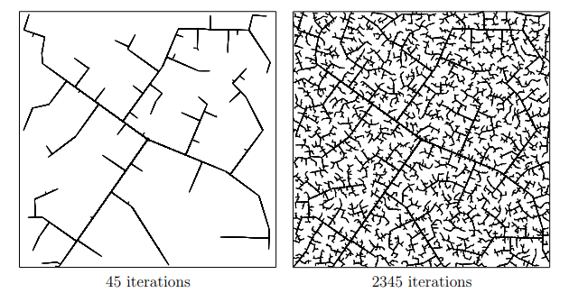
Two sample trees generated by the RRT Algorithm.
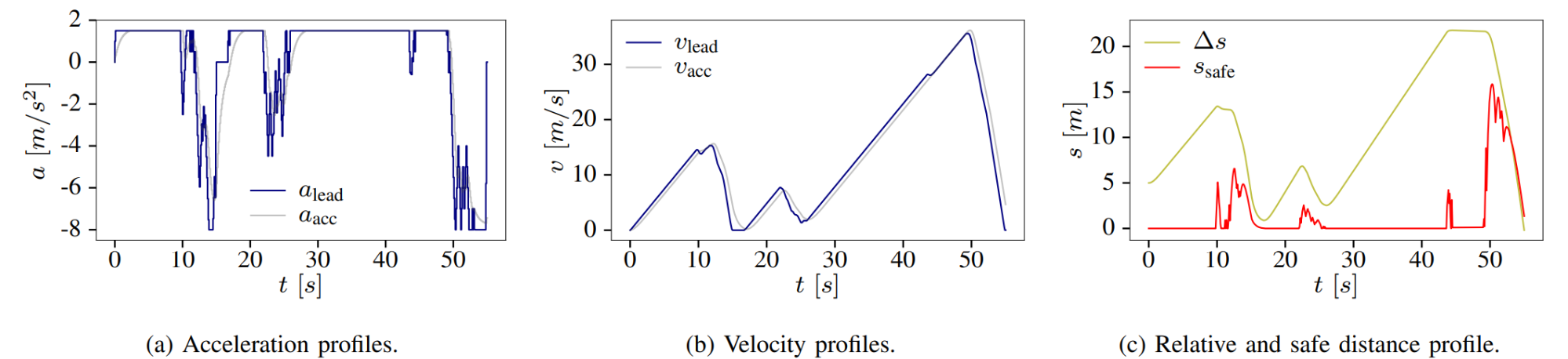
One of the most common path-planning algorithms that has been used for safety validation is the rapidly-exploring random tree (RRT) algorithm, depicted above13. In RRT, a space-filling tree is iteratively constructed by choosing disturbances that bring the environment into unexplored regions of the state space. The RRT algorithm has been used to find failures of an adaptive cruise control system14 where failures involved complex motion of the lead vehicle (shown below) that would be rarely discovered by traditional sampling techniques.
Sample failure of an adaptive cruise control system.
Many path planning approaches were designed to be used with white-box systems and environments where dynamics and gradient information is available. When applied to black-box safety validation, these algorithms need to be adapted to forego the use of such information. For example, in multiple shooting methods, a trajectory is constructed through disjoint segments, which are then joined using gradient descent. In the absence of gradient information, a black-box multiple shooting method was developed that connected segments by successively refining the segment inputs and outputs through full trajectory rollouts15.
Reinforcement Learning
The safety validation problem can be further simplified if we describe it as a Markov decision process where the next state of the environment is only a function of the current state and disturbance. The Markov assumption allows us to select disturbances based only on the current state and apply reinforcement learning (RL) algorithms such as Monte Carlo tree search (MCTS), and deep RL algorithms such as Deep Q-Networks or Proximal Policy Optimization.
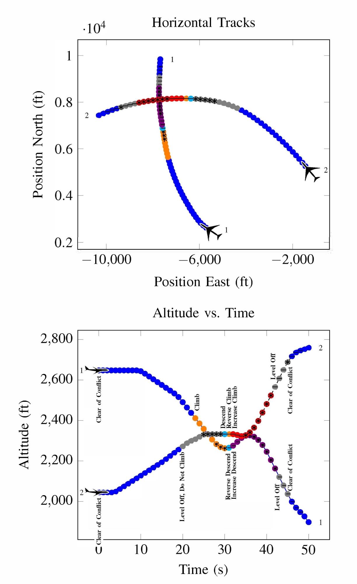
Monte Carlo tree search is similar to RRT in that a search tree is iteratively created to find disturbance trajectories that end in failure. Unlike RRT, however, MCTS is designed for use with black-box systems. The trajectories are always rolled out from the initial state of the simulator and the search is guided by a reward function rather than a coverage of the state space. These modifications allow MCTS to be applied in the most information-poor environments. Lee et. al16 used MCTS to find failures of an aircraft collision avoidance system (an example failure is depicted below) where they had no access to the simulator state and could only control actions through a pseudorandom seed. This approach may be preferred when organizations don’t want to expose any aspect of the functioning of their system.
Deep RL has seen a lot of success in recent years due to its ability to solve problems with large state spaces, complex dynamics, and large action spaces. The success of deep RL is due to the large representational capacity of neural networks and advanced optimization techniques, which make it a natural choice as a safety validation algorithm. For example, it has been used to find failures of autonomous driving policies17 where the state and action spaces are large and continuous—attributes that are difficult for other algorithms to handle well. A sample failure of an autonomous driving policy is demonstrated below18.
(Left) Sample failure of an aircraft collision avoidance system, (right) sample failure of a driving policy.
Optimization, path-planning and RL approaches all lend themselves to solving the problems of falsification and most likely failure analysis. However, when we need to evaluate the failure probability of a system, importance sampling approaches should be used.
Importance Sampling
The final set of approaches are well-suited for the task of estimating the probability of failure of the system from many failure examples. Importance sampling approaches seek to learn a sampling distribution that reliably produces failures and can be used to estimate the probability of failure with the minimal number of samples. Some common approaches are the cross-entropy method19, multilevel splitting20, supervised learning21, and approximate dynamic programming22.
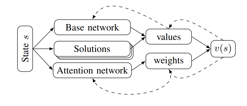
Most importance sampling approaches suffer the same drawback as optimization-based approaches: they are constructing a distribution across the entire disturbance trajectory . If we can invoke the Markov assumption, however, then we can construct a good sampling distribution based only on the current state using dynamic programming. However, the downside to dynamic programming is its inability to scale to large state spaces and thus complex scenarios. Our recent work23 shows that we can overcome this scalability problem by decomposing the system into subproblems and combining the subproblem solutions. For example, in an autonomous driving scenario, each adversarial agent on the road is paired with the ego vehicle to create a smaller safety validation problem with just two agents. Each of these problems are solved and then recombined using a neural network based on the Attend, Adapt and Transfer (A2T) architecture24. The combined solution is then refined using simulations of the full scenario. The decomposition strategy, network architecture and a sample failure for a 5-agent driving scenario is shown below. These types of hybrid approaches will be required to solve the most challenging safety validation problems.
(Left) Decomposition into pairwise subproblems, each involving the blue ego vehicle. (Right) The network used to fuse the subproblem solutions based on A2T.
Sample failure for an autonomous driving policy in a complex environment.
The Future
The validation of complex and safety-critical autonomous systems will likely involve many different techniques throughout the system design cycle, and black-box safety validation algorithms will play a crucial role. In particular, black-box algorithms are useful to the engineers who design safety-critical systems as well as third-party organizations that wish to validate the safety of such systems for regulatory or risk-assessment purposes. Although this post reviews many algorithms that will be of practical use for the validation of safety-critical autonomous systems, there are still areas that require more investigation. For example, we would like to be able to answer the question: if no failure has been found, how sure are we that the system is safe? This will require the development of algorithms that have formal or probabilistic guarantees of convergence. Scalability also remains a significant challenge. Autonomous systems can encounter a wide range of complex interactions, so safety validation algorithms must be able to efficiently discover failures in the most complex scenarios. The algorithms presented in this survey are a promising step toward safe and beneficial autonomy.
Acknowledgements
Many thanks to Michelle Lee, Andrey Kurenkov, Robert Moss, Mark Koren, Ritchie Lee, and Mykel Kochenderfer for comments and edits on this blog post.
Shalev-Shwartz, Shai, et al. “On a formal model of safe and scalable self-driving cars.” arXiv preprint arXiv:1708.06374 (2017). ↩
Bouton, Maxime, et al. “Reinforcement learning with probabilistic guarantees for autonomous driving.” arXiv preprint arXiv:1904.07189 (2019). ↩
Katz, Guy, et al. “Reluplex: An efficient SMT solver for verifying deep neural networks.” International Conference on Computer Aided Verification. Springer, 2017. ↩
Fainekos, Georgios E., et al. “Robustness of temporal logic specifications for continuous-time signals.” Theoretical Computer Science 410.42 (2009): 4262-4291. ↩
Mathesen, Logan, et al. “Falsification of cyber-physical systems with robustness uncertainty quantification through stochastic optimization with adaptive restart.” International Conference on Automation Science and Engineering (CASE). IEEE, 2019. ↩
M. J. Kochenderfer and T. A. Wheeler, Algorithms for optimization. MIT Press, 2019. ↩
Abbas, Houssam, et al. “Probabilistic temporal logic falsification of cyber-physical systems.” ACM Transactions on Embedded Computing Systems (TECS) 12.2s (2013): 1-30. ↩
Zou, Xueyi, et al. “Safety validation of sense and avoid algorithms using simulation and evolutionary search.” International Conference on Computer Safety, Reliability, and Security. Springer, 2014. ↩
Mullins, Galen E., et al. “Adaptive generation of challenging scenarios for testing and evaluation of autonomous vehicles.” Journal of Systems and Software 137 (2018): 197-215. ↩
Annapureddy, Yashwanth Singh Rahul, et al. “Ant colonies for temporal logic falsification of hybrid systems.” Annual Conference on IEEE Industrial Electronics Society (IECON). IEEE, 2010. ↩
Corso, Anthony, et al. “Interpretable safety validation for autonomous vehicles.” To appear in International Conference on Intelligent Transportation Systems (ITSC). IEEE, 2020. ↩
Nahhal, Tarik, et al. “Test coverage for continuous and hybrid systems.” International Conference on Computer Aided Verification. Springer, Berlin, Heidelberg, 2007. ↩
LaValle, Steven M. Planning algorithms. Cambridge University Press, 2006. ↩
Koschi, Markus, et al. “Computationally efficient safety falsification of adaptive cruise control systems.”_ Intelligent Transportation Systems Conference (ITSC)_. IEEE, 2019. ↩
Zutshi, Aditya, et al. “Multiple shooting, cegar-based falsification for hybrid systems.” International Conference on Embedded Software. 2014. ↩
Lee, Ritchie, et al. “Adaptive stress testing of airborne collision avoidance systems.” Digital Avionics Systems Conference (DASC). IEEE, 2015. ↩
Koren, Mark, et al. “Adaptive stress testing for autonomous vehicles.” Intelligent Vehicles Symposium (IV). IEEE, 2018. ↩
Corso, Anthony, et al. “Adaptive stress testing with reward augmentation for autonomous vehicle validation.” Intelligent Transportation Systems Conference (ITSC). IEEE, 2019. ↩
O’Kelly, Matthew, et al. “Scalable end-to-end autonomous vehicle testing via rare-event simulation.” Advances in Neural Information Processing Systems. 2018. ↩
Norden, Justin, et al. “Efficient black-box assessment of autonomous vehicle safety.” arXiv preprint arXiv:1912.03618 (2019). ↩
Uesato, Jonathan, et al. “Rigorous agent evaluation: An adversarial approach to uncover catastrophic failures.” arXiv preprint arXiv:1812.01647 (2018). ↩
Corso, Anthony, et al. “Scalable autonomous vehicle safety validation through dynamic programming and scene decomposition.” To appear in International Conference on Intelligent Transportation Systems (ITSC). IEEE, 2020. ↩
Corso, Anthony, et al. “Scalable autonomous vehicle safety validation through dynamic programming and scene decomposition.” To appear in International Conference on Intelligent Transportation Systems (ITSC). IEEE, 2020. ↩
Rajendran, Janarthanan, et al. “Attend, adapt and transfer: Attentive deep architecture for adaptive transfer from multiple sources in the same domain.” arXiv preprint arXiv:1510.02879 (2015). ↩
Nobody likes chores — can we build robots to do these chores, such as
cooking, for us? A common paradigm for training agents to perform
various tasks is to train a separate agent on each task, completely from
scratch, with reinforcement learning. However, training a robot to cook
with reinforcement learning from scratch in each person’s home would
completely fail, as it would result in many disasters (e.g., kitchen
fires), would require a lot of supervision from each person to reward
the robot for successfully cooking meals, and would take a long time
(learning even simple tasks from scratch can take reinforcement learning
agents millions of attempts).
Instead, it would be ideal if we could train a robot to be able to
quickly adapt to various home kitchens, after first training in many
kitchens in a robot chef factory. Intuitively, this should be possible
since different tasks and environments share considerable structure
(e.g., cooking pizza in one kitchen is similar to cooking a hamburger in
another kitchen), which can make learning each task easier and more
efficient.
Fortunately, meta-reinforcement learning seeks this exact goal of
training agents to adapt to new tasks from very few interactions on the
new task, after first training on many similar tasks. So, why aren’t
robots cooking in our kitchens today? To answer this question, we’ll
turn our attention to the problem of meta-exploration: how to best
spend these few interactions exploring the new task. For example, in
order to adapt to a new kitchen, a robot chef should ideally spend its
few interactions exploring the new kitchen to find the ingredients,
which will allow it to later cook a meal (solve the task). In this blog
post, we’ll cover and solve two key challenges about
meta-exploration that keep humans in the kitchen.
First, we’ll show that existing meta-reinforcement learning
approaches suffer from a chicken-and-egg coupling problem:
learning to explore and find the ingredients only helps a robot
prepare a meal if it already knows how to cook, but the robot can
only learn to cook if it already knows where the ingredients are.
We’ll avoid this cyclic dependence of learning to explore and learning to
execute (solve the task) by proposing an objective to learn them
independently of each other.
Second, we’ll observe that the standard meta-reinforcement learning
problem setting expects robots to cook the correct meal by
trial-and-error, without even being told what meal to cook, which
unnecessarily complicates the meta-exploration problem. To avoid
this, we propose instruction-based meta-reinforcement learning,
where the robot receives instructions specifying what meal to
cook.
Standard Meta-Reinforcement Learning
Standard meta-RL setting.
Before we dive in, let’s review the standard meta-reinforcement learning
(meta-RL) problem statement. In meta-reinforcement learning, an agent
(e.g., a robot chef) trains on many tasks (different recipes) and
environments (different kitchens), and then must accomplish a new task
in a new environment during meta-testing. When presented with a new task
and environment, the agent is allowed to first spend an episode
exploring, gathering any necessary information (e.g., locating the
ingredients), before execution episodes, where the agent must accomplish
the task (e.g., cook a meal).
In more formal language, standard meta-RL considers a family of
problems, where each problem identifies a reward function
(e.g., cook a pizza) and transition dynamics
(e.g., a kitchen).
Using the terminology from Duan et al., 2016, we define a trial to consist of
several episodes in the same problem. The first episode is the exploration
episode, where the agent is allowed to gather information, without needing to
maximize returns. All subsequent episodes are execution episodes, where the
agent must accomplish the task. The goal is to maximize the returns achieved
during the execution episodes of meta-testing trials, after first training on
many trials during meta-training.
Decoupled Reward-free Exploration and Execution in Meta-Reinforcement Learning (DREAM)
A chicken-and-egg coupling problem. A common approach (Wang et al.,
2016, Duan et al., 2016) for the meta-exploration problem is to optimize
a recurrent policy that performs both exploration and execution episodes
end-to-end based on the execution episode rewards. The hope is to
capture the information learned during the exploration episode in the
recurrent policy’s hidden state, which will then be useful for
execution episodes. However, this leads to a chicken-and-egg coupling
problem, where learning good exploration behaviors requires already
having learned good execution behaviors and vice-versa, which prevents
such an approach from learning.
For example, if a robot chef fails to discover the locations of
ingredients in a kitchen (bad exploration), then it cannot possibly
learn how to cook (bad execution). On the other hand, if the robot does
not know how to cook (bad execution), then no matter what it does during
the exploration episode, it will still not successfully cook a meal,
making learning exploration challenging. Since robots can’t cook or
explore at the beginning of training, they get stuck in this local
optimum and have a hard time learning either.
The coupling problem. What came first: the chicken (good exploration) or
the egg (good execution)?
Avoiding the coupling problem with DREAM. To avoid the
chicken-and-egg coupling problem, we propose a method to break the
cyclic dependency between learning exploration and learning execution
behaviors, which we call DREAM. Intuitively, good exploration can be
learned by trying to recover the information necessary for executing
instructions. Therefore, from a high-level, DREAM consists of two main
steps: 1) simultaneously learn an execution policy independently from
exploration and learn what information is necessary for execution and 2)
learn an exploration policy to recover that information.
To answer the chicken-and-egg problem, DREAM manufactures its own egg,
and out comes the chicken.
More concretely, in the first step, we train an execution policy
conditioned on the problem identifier , which in the cooking example,
may either directly identify attributes of the kitchen (e.g., wall color
or ingredient locations), or simply be a unique identifier (e.g., a
one-hot) for each kitchen. This problem identifier (directly or
indirectly) encodes all the information necessary to solve tasks in the
kitchen, allowing the execution policy to learn independently from
exploration, which avoids the coupling problem. At the same time, our
goal in the first step is to identify only the information necessary for
executing instructions, and the problem identifier may also encode
extraneous information, such as the wall color. To remove this, we apply
an information bottleneck to obtain a bottlenecked representation ,
which we use for training an exploration policy .
In the second step, once we’ve obtained a bottleneck representation
that ideally contains only the information necessary for executing
instructions, we can train an exploration policy to recover this
information in the exploration episode. To do this, we roll-out the
exploration policy to obtain an episode and then reward the policy
based on how well this episode encodes the information contained in .
Roughly, this reward is the mutual information between the
bottlenecked representation and the episode .
DREAM meta-testing.
The problem identifier is easy to provide during meta-training by
simply assigning each problem a unique one-hot, but is typically
unavailable or unhelpful during meta-testing (e.g., if is a completely
new one-hot). This might seem concerning, since, during meta-training,
the execution policy conditions on , which requires knowing . However,
since the exploration policy is trained to produce exploration
trajectories that contain the same information as , we can directly
swap for at meta-test time by rolling out the exploration policy.
See our paper for the details!
Improving the standard meta-RL setting. A second meta-exploration
challenge concerns the meta-reinforcement learning setting itself.
While the above standard
meta-RL setting is a useful problem formulation, we observe two areas
that can be made more realistic. First, the standard setting requires
the agent to infer the task (e.g., the meal to cook) from reward
observations, which can be needlessly inefficient. In more realistic
situations, the user would just tell the agent what they want, instead.
Open and honest communication is important for your robots too.
Second, while the standard meta-RL setting leverages shared structure
between different problems (environment and task pairs), it does not
capture shared structure between different tasks in the same
environment. More concretely, the task is fixed across all episodes in a
trial, and in order to perform a new task (e.g., cook a new meal), the
agent requires another exploration episode, even when the underlying
environment (e.g., the kitchen) stays the same. Instead, an agent would
ideally be able to perform many tasks after a single exploration
episode. For example, after exploring the kitchen to find any
ingredients, an ideal robot chef would be able to then cook any meal
involving those ingredients, whereas an agent trained in the standard
meta-reinforcement learning setting would only be able to cook a single meal.
Dinner schedule according to a robot chef trained in the standard
meta-reinforcement learning setting.
These two areas can obscure the meta-exploration problem of how to
optimally spend the exploration episode, as the former requires
unnecessary exploration to infer the task, while the latter only
requires the agent to explore to discover information relevant to a
single task. While intuitively, the agent should spend the exploration
episode gathering useful information for later execution episodes, in
many cases, optimal exploration collapses to simply solving the task.
For example, the agent can only discover that the task is to cook pizza
by successfully cooking pizza and receiving positive rewards, only to do
the same thing again and again on future execution episodes. This can
make the exploration episode nearly useless.
Instruction-based meta-RL (IMRL). To make the meta-RL setting more
realistic, we propose a new setting called instruction-based meta-RL
(IMRL), which addresses the two above areas by (i) providing the agent
with instructions (e.g., “cook pizza” or a one-hot representation)
that specify the task during execution episodes and (ii) varying the
task by providing a different instruction on each execution episode.
Then, for example, after meta-training in different kitchens at a
factory, a robot chef could begin cooking many different meals specified
by a human in a new home kitchen, after a single setup period
(exploration episode).
Instruction-based meta-RL: The task, which changes each execution
episode, is conveyed to the agent via instructions. The environment
still stays the same within a trial.
Reward-free adaptation. In the standard meta-RL setting, the agent
requires reward observations during exploration episodes in order to
infer the task. However, by receiving instructions that specify the task
in IMRL, a further benefit is that the agent no longer requires observing
rewards to adapt to new tasks and environments. Concretely, IMRL enables
reward-free adaptation, where during meta-training, the agent uses reward
observations during execution episodes to learn to solve the task, but does
not observe rewards during exploration episodes. During meta-testing, the
agent never observes any rewards. This enables modeling real-world deployment
situations where gathering reward supervision is really expensive. For
example, a robot chef would ideally be able to adapt to a home kitchen without
any supervision from a human.
Is IMRL general? Importantly, setting the instruction to always be
some “empty” instruction recovers the standard meta-RL setting. In
other words, standard meta-RL is just IMRL, where the user’s desires
are fixed within a trial and the user says nothing for the instructions.
Therefore, algorithms developed for IMRL can also be directly applied to
the standard setting and vice-versa.
Results
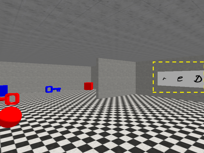
Sign reads blue.
Sign reads red.
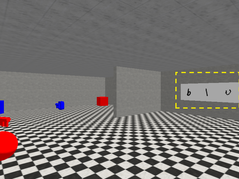
Sparse-reward 3D visual navigation. In one experiment from our
paper, we evaluate DREAM on the sparse-reward 3D visual navigation
problem family proposed by Kamienny et al., 2020 (pictured above), which
we’ve made harder by including a visual sign and more objects. We use
the IMRL setting with reward-free adaptation. During execution episodes,
the agent receives an instruction to go to an object: a ball, block or
key. The agent starts episodes on the far side of the barrier, and must
walk around the barrier to read the sign
(highlighted in yellow),
which in the two versions of the problem, either specify going to the blue or red version of the
object. The agent receives 80×60 RGB images as observations
and can turn left or right, or move forward. Going to the correct object gives
reward +1 and going to the wrong object gives reward -1.
DREAM learns near-optimal exploration and execution behaviors on this
task, which are pictured below. On the left, DREAM spends the
exploration episode walking around the barrier to read the sign, which
says blue. On the right, during an execution
episode, DREAM receives an instruction to go to the key. Since DREAM already
read that the sign said blue during the exploration
episode, it goes to the blue key.
Behaviors learned by DREAM
Exploration.
Execution: go to the key.
Comparisons. Broadly, prior meta-RL approaches fall into two main
groups: (i) end-to-end approaches, where exploration and execution are
optimized end-to-end based on execution rewards, and (ii) decoupled
approaches, where exploration and execution are optimized with separate
objectives. We compare DREAM with state-of-the-art approaches from both
categories. In the end-to-end category, we compare with:
RL12, the canonical
end-to-end approach, which learns a recurrent policy conditioned
on the entire sequence of past state and reward observations.
VariBAD3, which additionally adds auxiliary
loss functions to the hidden state of the recurrent policy to
predict the rewards and dynamics of the current problem. This can
be viewed as learning the belief state4, a
sufficient summary of all of its past observations.
IMPORT5, which additionally leverages the
problem identifier to help learn execution behaviors.
Additionally, in the decoupled category, we compare with:
PEARL-UB, an upperbound on PEARL6. We
analytically compute the expected rewards achieved by the optimal
problem-specific policy that explores with
Thompson sampling7 using the true posterior
distribution over problems.
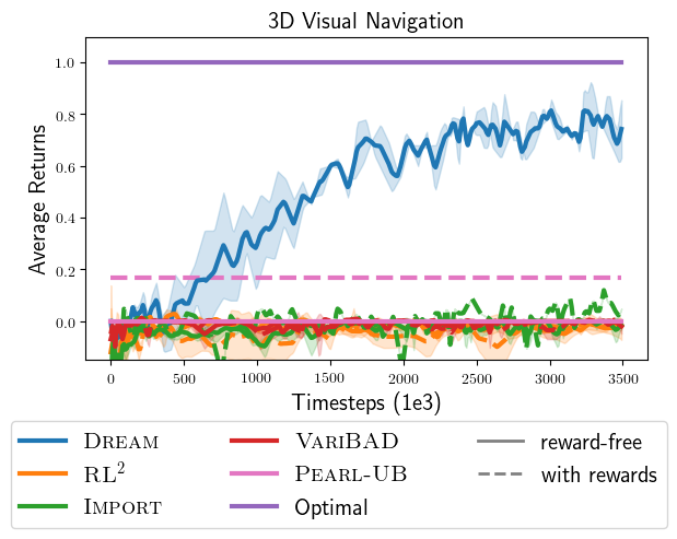
Quantitative results. Below, we plot the returns achieved by all
approaches. In contrast to DREAM, which achieves near-optimal returns,
we find that the end-to-end approaches never read the sign, and
consequently avoid all objects, in fear of receiving negative reward for
going to the wrong object. This happens even when they are allowed to
observe rewards in the exploration episode (dotted lines). Therefore,
they achieve no rewards, which is indicative of the coupling problem.
On the other hand, while existing approaches in the decoupled category
avoid the coupling problem, optimizing their objectives does not lead to
the optimal exploration policy. For example, Thompson sampling
approaches (PEARL-UB) do not achieve optimal reward, even with the
optimal problem-specific execution policy and access to the true
posterior distribution over problems. To see this, recall that Thompson
sampling explores by sampling a problem from the posterior distribution
and following the execution policy for that problem. Since the optimal
execution policy directly goes to the correct object, and never reads
the sign, Thompson sampling never reads the sign during exploration. In
contrast, a nice property of DREAM is that with enough data and
expressive-enough policy classes, it theoretically learns optimal
exploration and execution.
Training curves with (dotted lines) and without (solid lines) rewards
during exploration. Only DREAM reads the sign and solves the task. And
it does it without needing rewards during exploration!
Additional results. In our paper, we also evaluate DREAM on
additional didactic problems, designed to to answer the following
questions:
Can DREAM efficiently explore to discover only the information
required to execute instructions?
Can DREAM generalize to unseen instructions and environments?
Does DREAM also show improved results in the standard meta-RL
setting, as well as instruction-based meta-RL?
Broadly, the answer is yes to all of these questions. Check out our
paper for detailed results!
Conclusion
Summary. In this blog post, we tackled the problem of
meta-exploration: how to best gather information in a new environment in
order to perform a task. To do this, we examined and addressed two key
challenges.
First, we saw how existing meta-RL approaches that optimize both
exploration and execution end-to-end to maximize reward fall
prey to a chicken-and-egg problem. If the agent hasn’t learned to
explore yet, then it can’t gather key information (e.g., the
location of ingredients) required for learning to solve tasks
(e.g., cook a meal). On the other hand, if the agent hasn’t
learned to solve tasks yet, then there’s no signal for learning to
explore, as it’ll fail to solve the task no matter what. We
avoided this problematic cycle by proposing a decoupled
objective (DREAM), which learns to explore and learns to solve
tasks independently from each other.
Second, we saw how the standard meta-RL setting captures the notion
of adapting to a new environment and task, but requires the agent
to unnecessarily explore to infer the task (e.g., what meal to
cook) and doesn’t leverage the shared structure between different
tasks in the same environment (e.g., cooking different meals in
the same kitchen). We addressed this by proposing
instruction-based meta-RL (IMRL), which provides the agent with an
instruction that specifies the task and requires the agent to
explore and gather information useful for many tasks.
DREAM and IMRL combine quite nicely: IMRL enables reward-free adaptation
in principle, and DREAM achieves it in practice. Other state-of-the-art
approaches we tested weren’t able to achieve reward-free adaptation, due
to the chicken-and-egg coupling problem.
What’s next? There’s a lot of room for future work — here are a
few directions to explore.
More sophisticated instruction and problem ID representations.
This work examines the case where the instructions and problem IDs
are represented as unique one-hots, as a proof of concept. Of
course, in the real world, instructions and problem IDs might be
better represented with natural language, or images (e.g., a
picture of the meal to cook).
Applying DREAM to other meta-RL settings. DREAM applies generally
to any meta-RL setting where some information is conveyed to the
agent and the rest must be discovered via exploration. In this
work, we studied two such instances — in IMRL, the instruction
conveys the task and in the standard meta-RL setting, everything
must be discovered via exploration — but there are other settings
worth examining, too. For example, we might want to convey
information about the environment to the agent, such as the
locations of some ingredients, or that the left burner is broken,
so the robot chef should use the right one.
Seamlessly integrating exploration and execution. In the most
commonly studied meta-RL setting, the agent is allowed to first
gather information via exploration (exploration episode) before
then solving tasks (execution episodes). This is also the setting
we study, and it can be pretty realistic. For example, a robot
chef might require a setup phase, where it first explores a home
kitchen, before it can start cooking meals. On the other hand, a
few works, such as Zintgraf et al., 2019, require the agent to
start solving tasks from the get-go: there are no exploration
episodes and all episodes are execution episodes. DREAM can
already operate in this setting, by just ignoring the rewards and
exploring in the first execution episode, and trying to make up
for the first execution episode with better performance in later
execution episodes. This works surprisingly well, but it’d be nice
to more elegantly integrate exploration and execution.
Many thanks to Andrey Kurenkov
for comments and edits on this blog post!
The icons used in the above figures were made by Freepik, ThoseIcons,
dDara, mynamepong, Icongeek26, photo3idea_studio and Vitaly Gorbachev
from flaticon.com.
Y. Duan, J. Schulman, X. Chen, P. L. Bartlett, I. Sutskever, and P. Abbeel. RL2: Fast reinforcement learning via slow reinforcement learning. arXiv preprint arXiv:1611.02779, 2016. ↩
J. X. Wang, Z. Kurth-Nelson, D. Tirumala, H. Soyer, J. Z. Leibo, R. Munos, C. Blundell, D. Kumaran, and M. Botvinick. Learning to reinforcement learn. arXiv preprint arXiv:1611.05763, 2016. ↩
L. Zintgraf, K. Shiarlis, M. Igl, S. Schulze, Y. Gal, K. Hofmann, and S. Whiteson. VariBAD A very good method for bayes-adaptive deep RL via meta-learning. arXiv preprint arXiv:1910.08348, 2019. ↩
L. P. Kaelbling, M. L. Littman, and A. R. Cassandra. Planning and acting in partially observable stochastic domains. Artificial intelligence, 101(1):99–134, 1998. ↩
P. Kamienny, M. Pirotta, A. Lazaric, T. Lavril, N. Usunier, and L. Denoyer. Learning adaptive exploration strategies in dynamic environments through informed policy regularization. arXiv preprint arXiv:2005.02934, 2020. ↩
K. Rakelly, A. Zhou, D. Quillen, C. Finn, and S. Levine. Efficient off-policy meta-reinforcement learning via probabilistic context variables. arXiv preprint arXiv:1903.08254, 2019. ↩
W. R. Thompson. On the likelihood that one unknown probability exceeds another in view of the evidence of two samples. Biometrika, 25(3):285–294, 1933. ↩
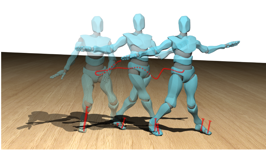
The European Conference on Computer Vision (ECCV) 2020 is being hosted virtually from August 23rd – 28th. We’re excited to share all the work from SAIL that’s being presented, and you’ll find links to papers, videos and blogs below. Feel free to reach out to the contact authors directly to learn more about the work that’s happening at Stanford!
Keywords: 3d human pose, 3d human motion, pose estimation, dynamics, physics-based, contact, trajectory optimization, character animation, deep learning
The International Conference on Machine Learning (ICML) 2020 is being hosted virtually from July 13th – July 18th. We’re excited to share all the work from SAIL that’s being presented, and you’ll find links to papers, videos and blogs below. Feel free to reach out to the contact authors directly to learn more about the work that’s happening at Stanford!
List of Accepted Papers
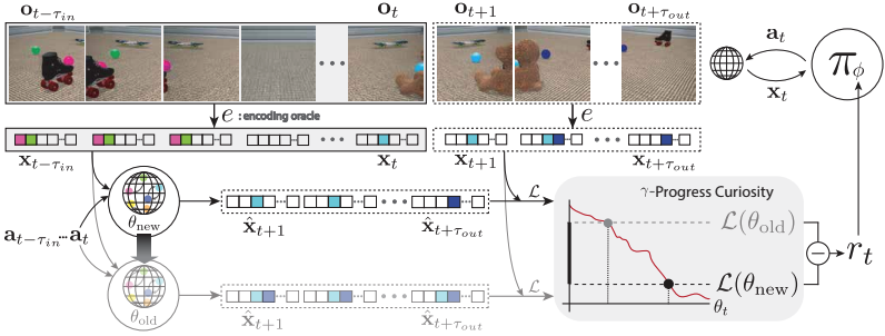
Active World Model Learning in Agent-rich Environments with Progress Curiosity
Authors: Kuno Kim, Megumi Sano, Julian De Freitas, Nick Haber, Daniel Yamins
Robotics: Science and Systems (RSS) 2020 is being hosted virtually from July 12th – June 16th. We’re excited to share all the work from SAIL and Stanford Robotics that’s being presented! Below you’ll find links to each paper, as well as the authors’ five-minute presentation of their research. Feel free to reach out to the contact authors directly to learn more about what’s happening at Stanford.
In addition to these papers, SAIL students and faculty are involved in organizing several workshops at RSS. We invite you to attend these workshops, where you can hear from amazing speakers, interact, and ask questions! Workshop attendance is completely virtual: we provide information and links to these workshops at the bottom of this post.
Prerecorded Talks by: Stefan Schaal. Karen Liu, Sangbae Kim, Andy Zeng, David Hsu, Leslie Kaebling, Nicolas Heess, Angela Schoellig
Live Events on July 12th (PDT): Panels from 09:00 AM – 10:00 AM and 05:00 PM – 06:00 PM | Retrospective sessions from 10:00 AM – 11:00 AM and 04:00 PM – 05:00 PM
Prerecorded Talks by: Anca Dragan, Maya Cakmak, Yuke Zhu, Byron Boots, Abhinav Gupta, Oliver Kroemer
Live Events on July 12th (PDT): Paper discussions from 9:00 AM – 10:30 AM | Virtual coffee break from 10:30 AM – 11:00 AM | Panel from 11:00 AM – 1:30 PM
Organizers: Scott Niekum, Akanksha Saran, Yuchen Cui, Nick Walker, Andreea Bobu, Ajay Mandlekar, Danfei Xu
The 58th annual meeting of the Association for Computational Linguistics is being hosted virtually this week. We’re excited to share all the work from SAIL that’s being presented, and you’ll find links to papers, videos and blogs below. Feel free to reach out to the contact authors directly to learn more about the work that’s happening at Stanford!
List of Accepted Papers
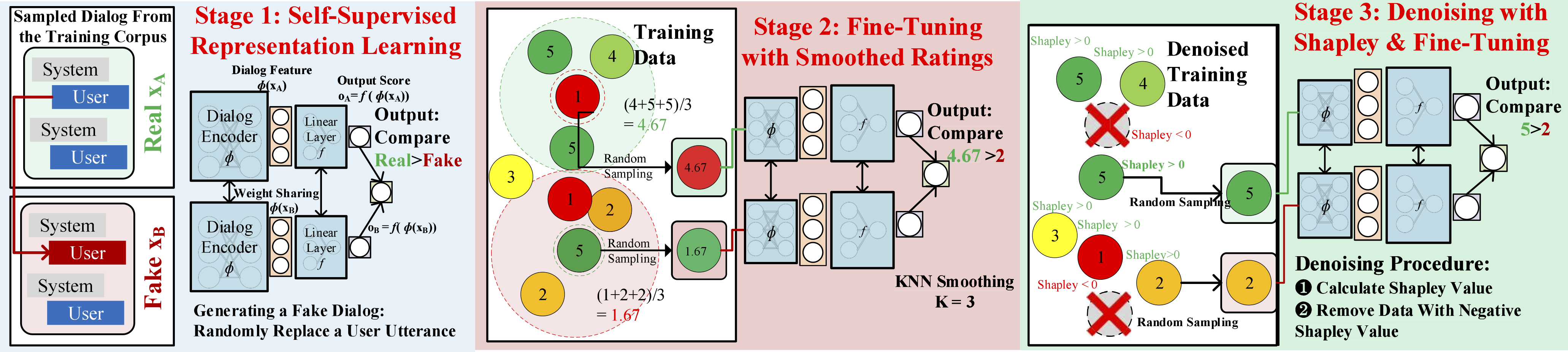
Beyond User Self-Reported Likert Scale Ratings: A Comparison Model for Automatic Dialog Evaluation
Authors: Weixin Liang, James Zou, Zhou Yu
Contact: wxliang@stanford.edu
Keywords: dialog, automatic dialog evaluation, user experience
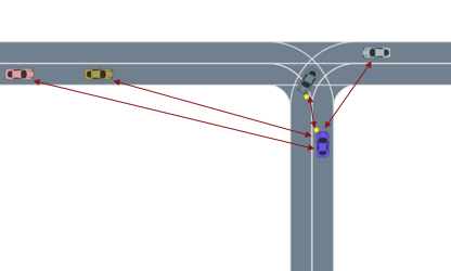
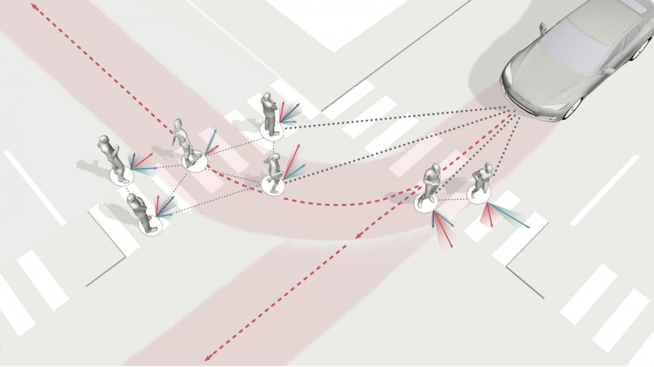
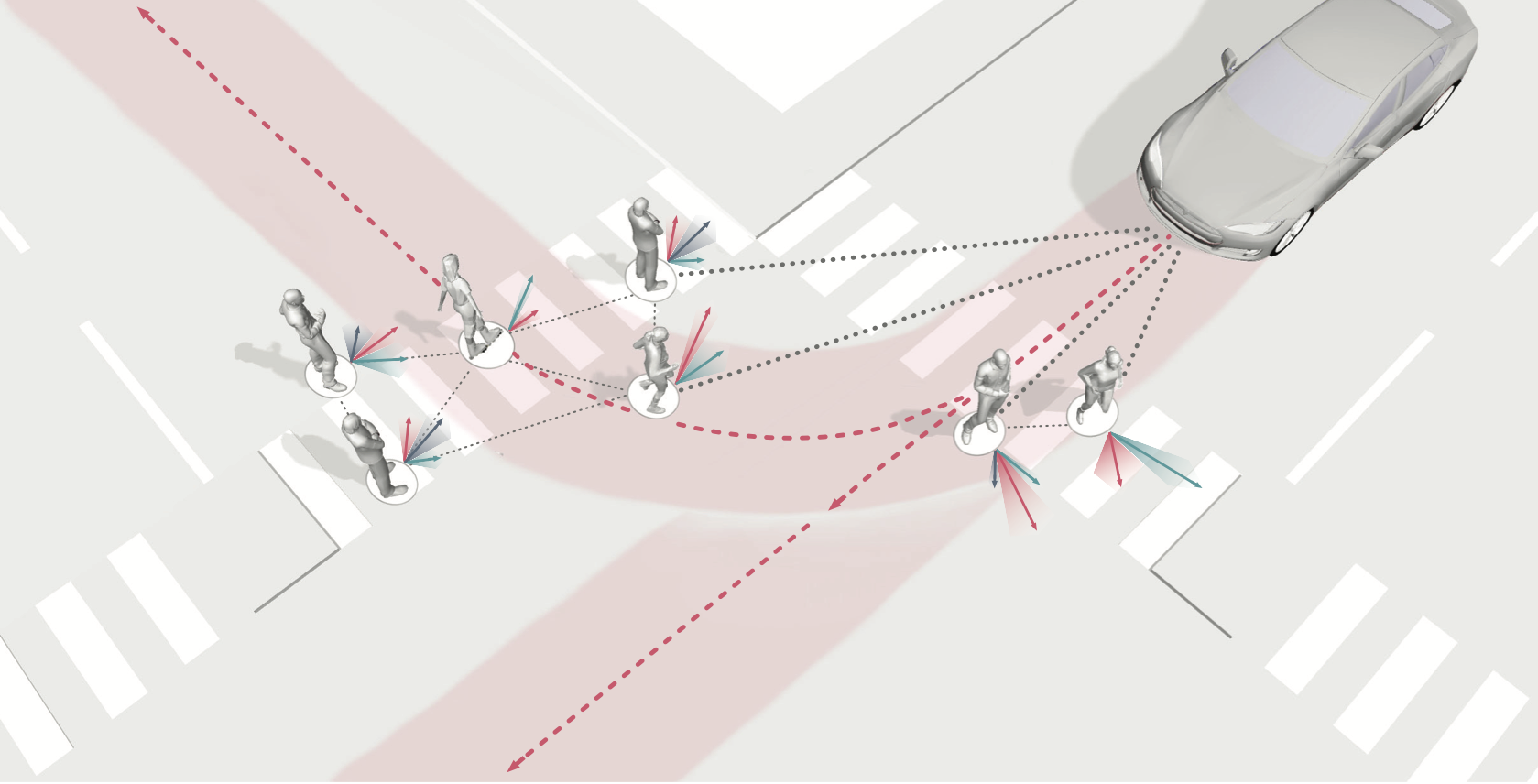
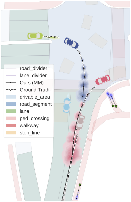
Merging into traffic is one of the most common day-to-day maneuvers we perform as drivers, yet still poses a major problem for self-driving vehicles. The reason that humans can naturally navigate through many social interaction scenarios, such as merging in traffic, is that they have an intrinsic capacity to reason about other people’s intents, beliefs, and desires, using such reasoning to predict what might happen in the future and make corresponding decisions1. However, many current autonomous systems do not use such proactive reasoning, which leads to difficulties when deployed in the real world. For example, there have been numerous instances of self-driving vehicles failing to merge into traffic, getting stuck in intersections, and making unnatural decisions that confuse others. As a result, imbuing autonomous systems with the ability to reason about other agents’ actions could enable more informed decision making and proactive actions to be taken in the presence of other intelligent agents, e.g., in human-robot interaction scenarios. Indeed, the ability to predict other agents’ behaviors (also known as multi-agent behavior prediction) has already become a core component of modern robotic systems. This holds especially true in safety-critical applications such as autonomous vehicles, which are currently being tested in the real world and targeting widespread deployment in the near future2. The diagram below illustrates a scenario where predicting the motion of other agents may help inform an autonomous vehicle’s path planning and decision making. Here, an autonomous vehicle is deciding whether to stay put or continue driving, depending on surrounding pedestrian movement. The red paths indicate future navigational plans for the vehicle, depending on its eventual destination.
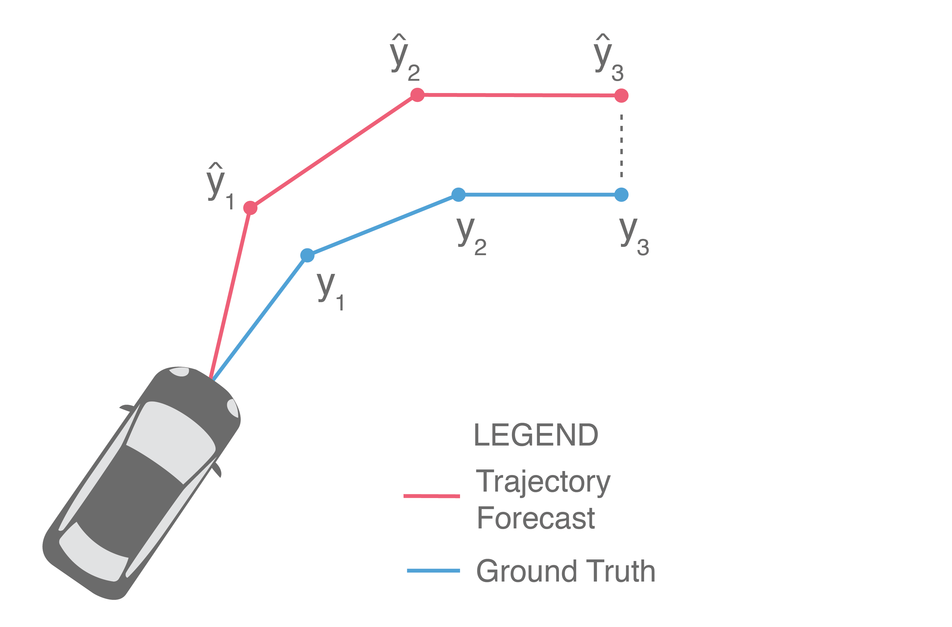
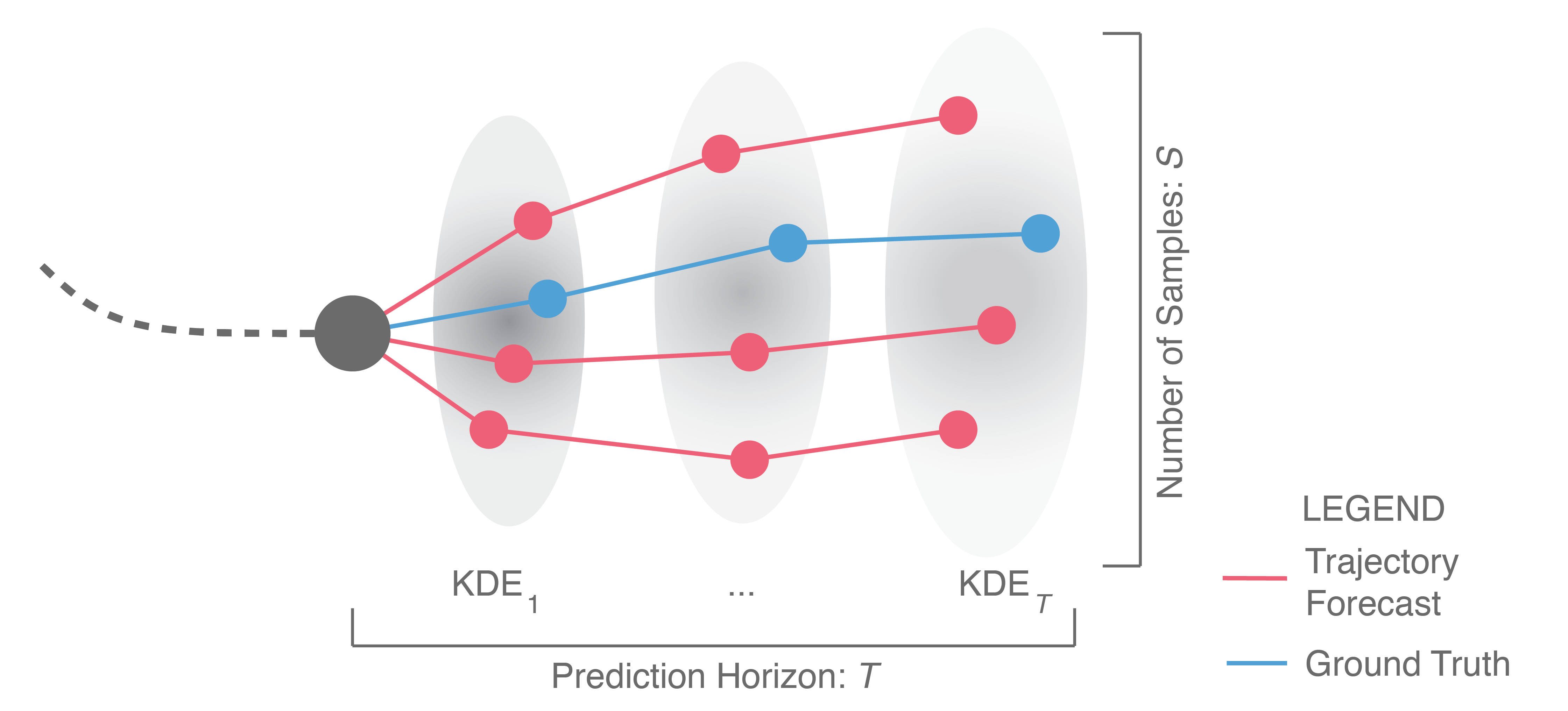
At a high level, trajectory forecasting is the problem of predicting the path (trajectory) that some sentient agent (e.g., a bicyclist, pedestrian, car driver, or bus driver) will move along in the future given the trajectory that agent moved along in the past. In scenarios with multiple agents, we are also given their past trajectories, which can be used to infer how they interact with each other. Trajectories of length are usually represented as a sequence of positional waypoints (e.g., GPS coordinates). Since we aim to make good predictions, we evaluate methods by some metric that compares the predicted trajectory against the actual trajectory the agent takes (denoted earlier as ).
In this post, we will dive into methods for trajectory forecasting, building a taxonomy along the way that organizes approaches by their methodological choices and output structures. We will discuss common evaluation schemes, present new ones, and suggest ways to compare otherwise disparate approaches. Finally, we will highlight shortcomings in existing methods that complicate their integration in downstream robotic use cases. Towards this end, we will present a new approach for trajectory forecasting that addresses these shortcomings, achieves state-of-the-art experimental performance, and enables new avenues of deployment on real-world autonomous systems.
1. Methods for Multi-Agent Trajectory Forecasting
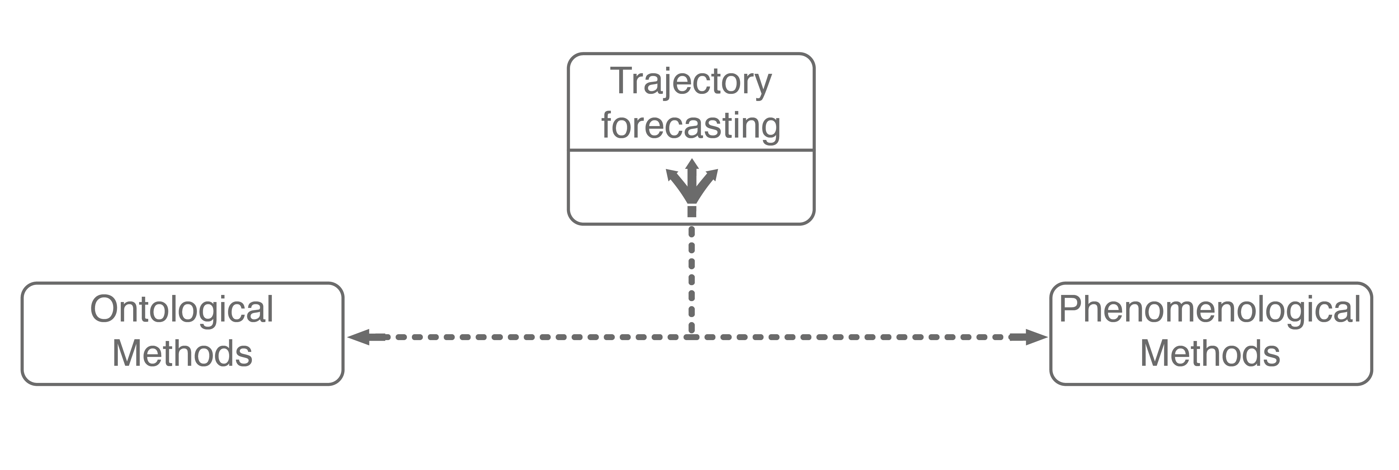
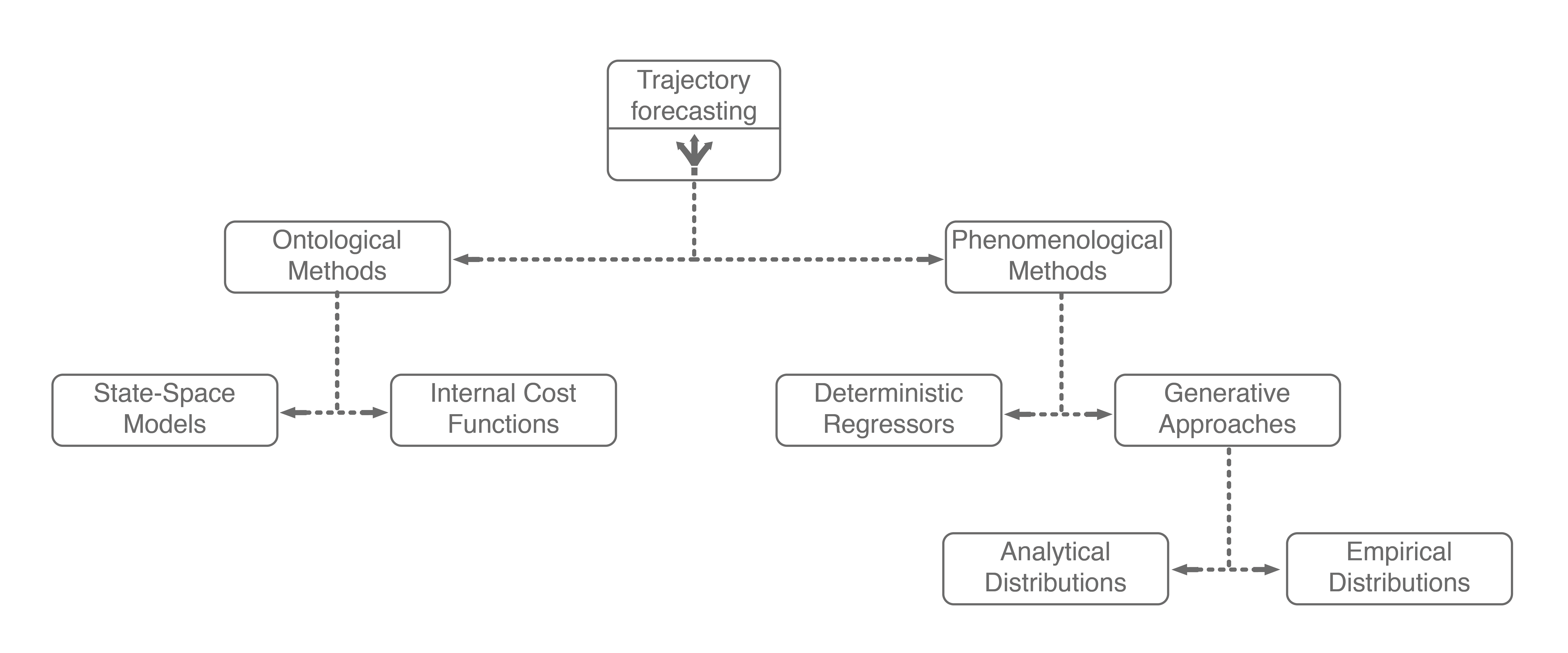
There are many approaches for multi-agent trajectory forecasting, ranging from classical, physics-based models to deterministic regressors to generative probabilistic models3. To explore them in a structured manner, we will first group methods by the assumptions they make followed by the technical approaches they employ, building a taxonomy of trajectory forecasting methodologies along the way.
The first major assumption that approaches make is about the structure, if any, the problem possesses. In trajectory forecasting, this is manifested by approaches being either ontological or phenomenological. Ontological approaches (sometimes referred to as theory of mind) generally postulate (assume) some structure about the problem, whether that be a set of rules that agents follow or rough formulations of agents’ internal decision-making schemes. Phenomenological approaches do not make such assumptions, instead relying on a wealth of data to gleam agent behaviors without reasoning about underlying motivations.
1.1. Ontological Approaches
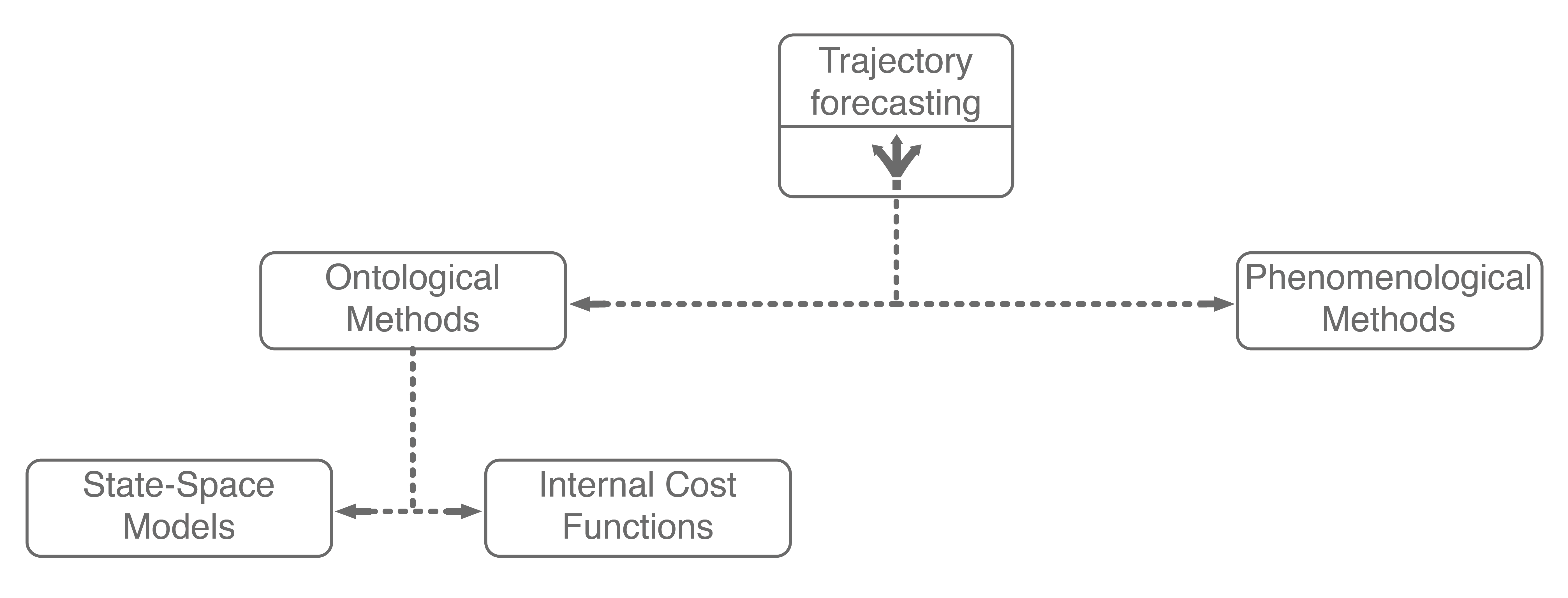
One of the simplest (and sometimes most effective) approaches for trajectory forecasting is classical mechanics. Usually, one assumes that they have a model that can predict the agent’s future state (also known as a dynamics model). With a dynamics model, one can predict the state (e.g., position, velocity, acceleration) of the agent several timesteps into the future. Such a simple approach is remarkably powerful, sometimes outperforming state-of-the-art approaches on real-world pedestrian modeling tasks4. However, pure dynamics integration alone does not account for the topology of the environment or interactions among agents, both of which are dominant effects. There have since been many approaches that mathematically formulate and model these interactions, exemplary methods include the intelligent driver model, MOBIL model, and Social Forces model.
More recently, inverse reinforcement learning (IRL) has emerged as a major ontological approach for trajectory forecasting. Given a set of agent trajectories in a scene , IRL attempts to learn the behavior and motivations of the agents. In particular, IRL formulates the motivation of an agent (e.g., crossing a sidewalk or turning right) with a mathematical formula, referred to as the reward function, shown below.
where refers to the reward value at a specific state (e.g., position, velocity, acceleration), is a set of weights to be learned, and is a set of extracted features that characterize the state . Thus, the IRL problem is to find the best weights . The main idea here is that solving a reinforcement learning problem with a successfully-learned reward function would yield a policy that matches , the original agent trajectories.
Unfortunately, there can be many such reward functions under which the original demonstrations are recovered. Thus, we need a way to choose between possible reward functions. A very popular choice is to pick the reward function with maximum entropy. This follows the principle of maximum entropy, which states that the most appropriate distribution to model a given set of data is the one with highest entropy among all feasible possibilities5. A reason why one would want to do this is that maximizing entropy minimizes the amount of prior information built into the model; there is less risk of overfitting to a specific dataset. This is named Maximum Entropy (MaxEnt) IRL, and has seen widespread use in modeling real-world navigation and driving behaviors.
To encode this maximum entropy choice into the IRL formulation from above, trajectories with higher rewards are valued exponentially more. Formally,
This distribution over paths also gives us a policy which can be sampled from. Specifically, the probability of an action is weighted by the expected exponentiated rewards of all trajectories that begin with that action.
Wrapping up, ontological approaches provide a structured method for learning how sentient agents make decisions. Due to their strong structural assumptions, they are both very sample-efficient (there are not many parameters to learn), computationally-efficient to optimize, and generally easier to pair with decision making systems (e.g., game theory). However, these strong structural assumptions also limit the maximum performance that an ontological approach may achieve. For example, what if the expert’s actual reward function was non-linear, had different terms than the assumed reward function, or was non-Markovian (i.e., had a history dependency)? In these cases, the assumed model would necessarily underfit the observed data. Further, data availability is growing at an exponential rate, with terabytes of autonomous driving data publicly being released every few months (companies have access to orders of magnitude more internally). With so much data, it becomes natural to consider phenomenological approaches6, which form the other main branch of our trajectory forecasting taxonomy.
Including these two ontological approaches in our trajectory forecasting taxonomy yields the above tree. Next, we will dive into mainline phenomenological approaches.
1.2. Phenomenological Approaches
Phenomenological approaches are methods that make minimal assumptions about the structure of agents’ decision-making process. Instead, they rely on powerful general modeling techniques and a wealth of observation data to capture the kind of complexity encountered in environments with multiple interacting agents.
There have been a plethora of data-driven approaches for trajectory forecasting, mainly utilizing regressive methods such as Gaussian Process Regression (GPR)7 and deep learning, namely Long Short-Term Memory (LSTM) networks8 and Convolutional Neural Networks (CNNs)9, to good effect. Of these, LSTMs generally outperform GPR methods and are faster to evaluate online. As a result, they are commonly found as a core component of human trajectory models10. The reason why LSTMs perform well is that they are a purpose-built deep learning architecture for modeling temporal sequence data. Thus, practitioners usually model trajectory forecasting as a time series prediction problem and apply LSTM networks.
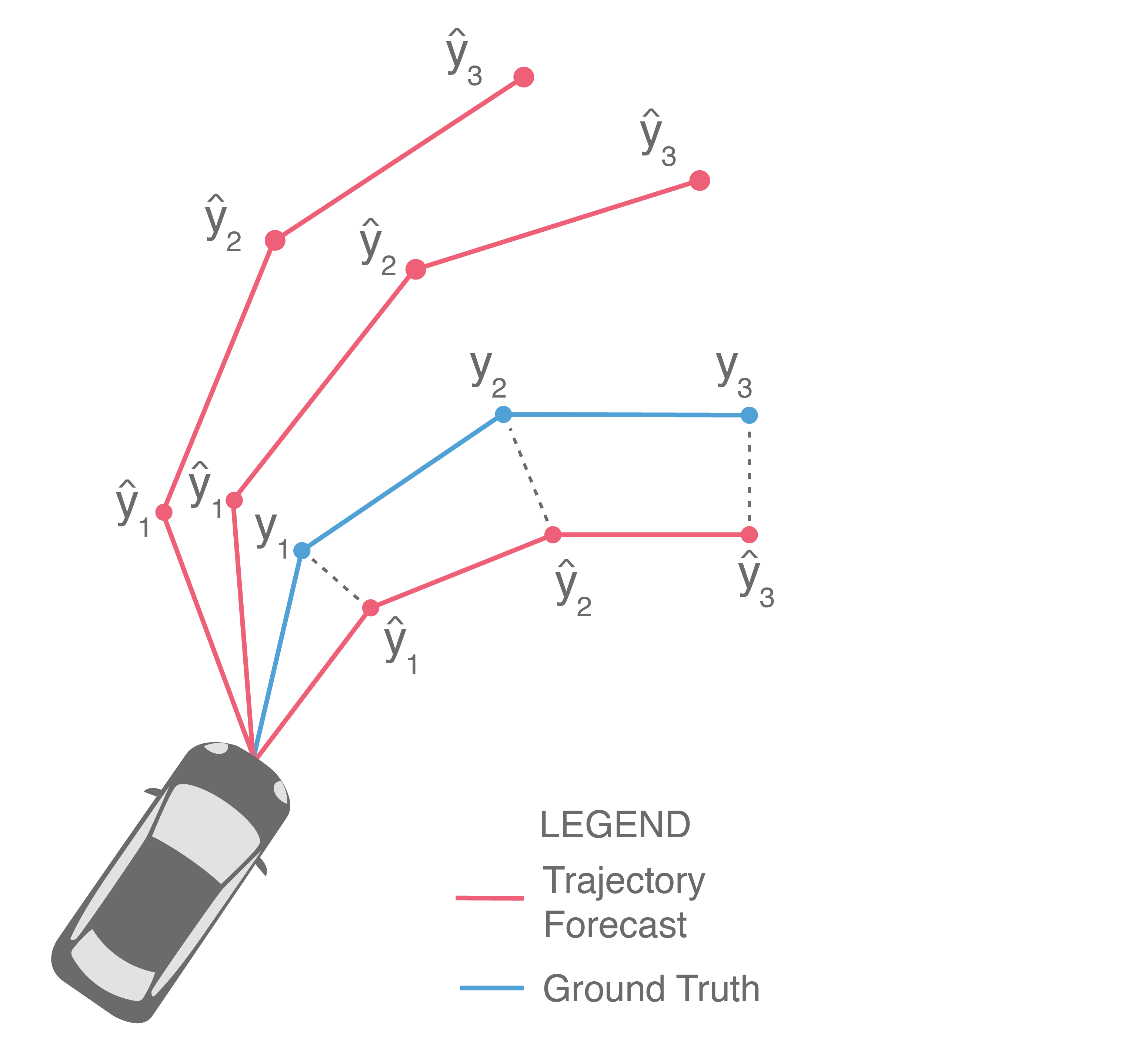
While these methods have enjoyed strong performance, there is a subtle point that limits their application to safety-critical problems such as autonomous driving: they only produce a single deterministic trajectory forecast. Safety-critical systems need to reason about many possible future outcomes, ideally with the likelihoods of each occurring, to make safe decisions online. As a result, methods that simultaneously forecast multiple possible future trajectories have been sought after recently.
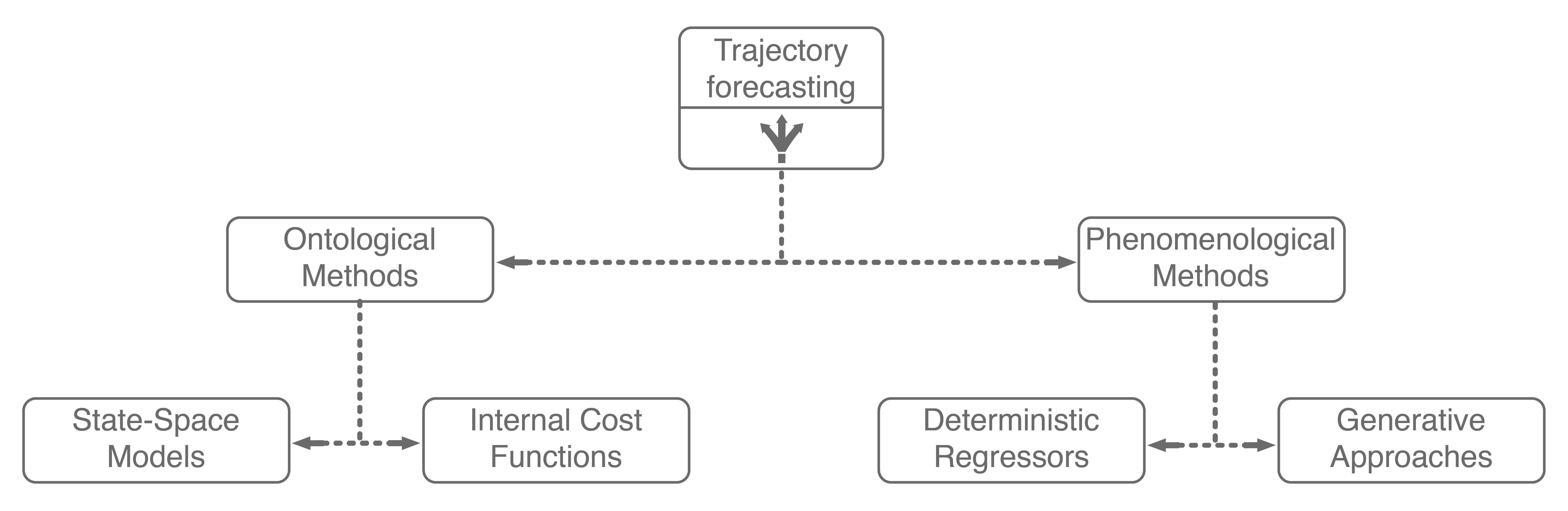
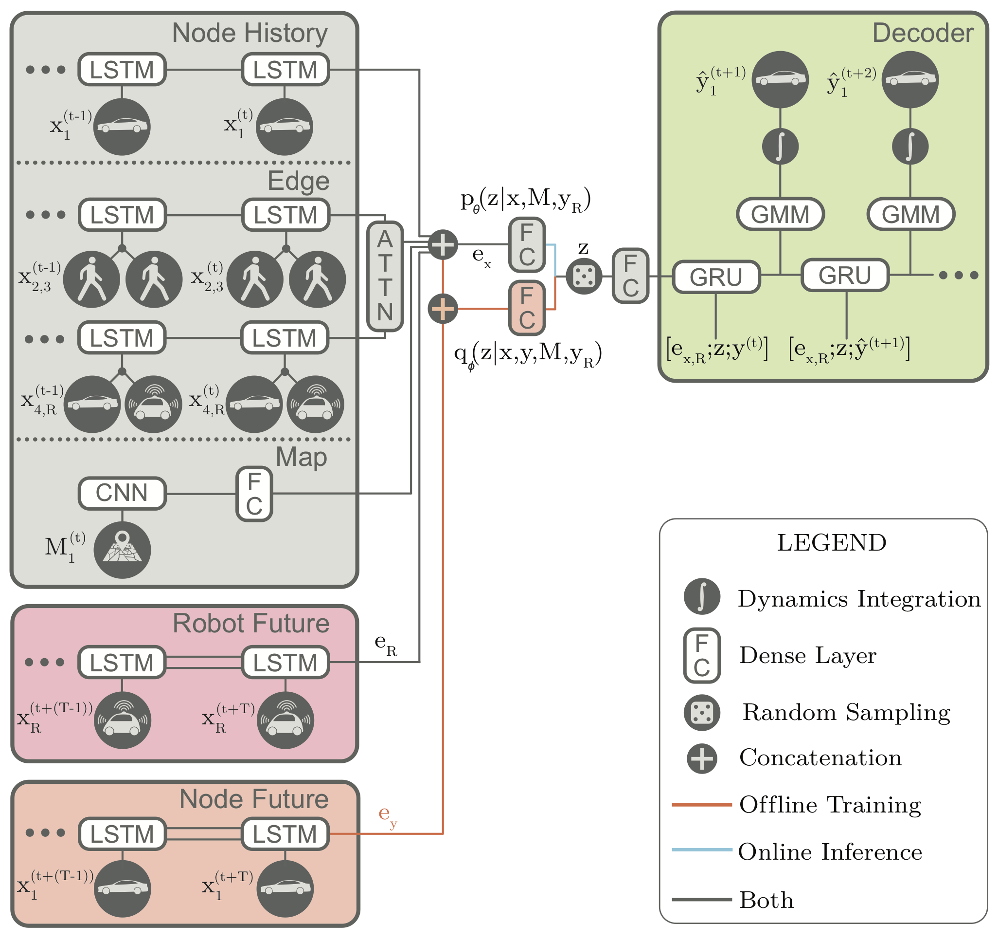
Generative approaches in particular have emerged as state-of-the-art trajectory forecasting methods due to recent advancements in deep generative models11. Notably, they have caused a paradigm shift from focusing on predicting the single best trajectory to producing a distribution of potential future trajectories. This is advantageous in autonomous systems as full distribution information is more useful for downstream tasks, e.g., motion planning and decision making, where information such as variance can be used to make safer decisions. Most works in this category use a deep recurrent backbone architecture (like an LSTM) with a latent variable model, such as a Conditional Variational Autoencoder (CVAE), to explicitly encode multimodality12, or a Generative Adversarial Network (GAN) to implicitly do so13. Common to both approach styles is the need to produce position distributions. GAN-based models can directly produce these and CVAE-based recurrent models usually rely on a bivariate Gaussian or bivariate Gaussian Mixture Model (GMM) to output position distributions. Including the two in our taxonomy balances out the right branch.
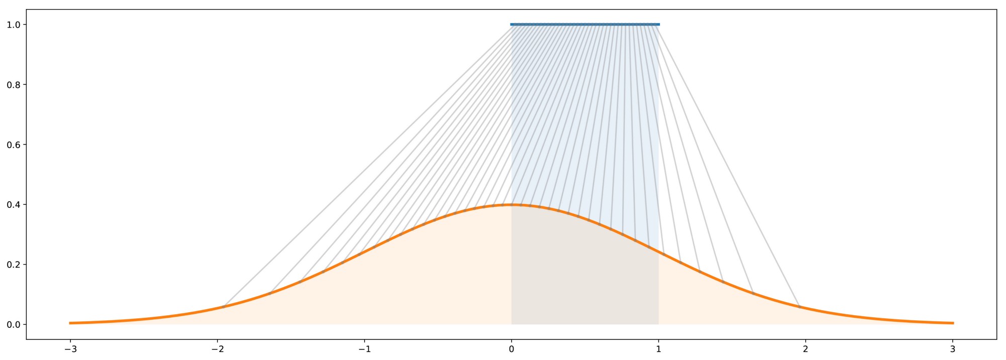
The main difference between GAN-based and CVAE-based approaches is in the form of their resulting output distribution. At a high level, GANs are generative models that generate data which, in aggregate, match the distribution of its training dataset . They achieve this by learning to map samples from a known distribution to samples of an unknown distribution for which we have samples, i.e., the training dataset. Intuitively, this is very similar to inverse transform sampling, which is a method for generating samples from any probability distribution given its cumulative distribution function. This is roughly illustrated below, where samples from a simple uniform distribution are mapped to a standard Gaussian distribution.
Thus, GANs can be viewed as learning an inverse transformation which maps a sample of a “simple” random variable to a sample of a “complex” random variable (conditioned on because that is the value being mapped to ). Thinking about this from the perspective of trajectory forecasting, is usually the trajectory history of the agent, information about neighboring agents, environmental information, etc. and is the trajectory forecast we are looking to output. Thus, it makes sense that one would want to produce predictions conditioned on past observations . However, this sampling-based structure also means that GANs can only produce empirical, and not analytical, distributions. Specifically, obtaining statistical properties like the mean and variance from a GAN can only be done approximately, through repeated sampling.
On the other hand, CVAEs tackle the problem of representing by decomposing it into subcomponents specified by the value of a latent variable . Formally,
Note that the sum in the above equation implies that is discrete (has finitely-many values). The latent variable can also be continuous, but there is work showing that discrete latent spaces lead to better performance (this also holds true for trajectory forecasting)14, so for this post we will only concern ourselves with a discrete . By decomposing in this way, one can produce an analytic output distribution. This is very similar to GMMs, which also decompose their desired distribution in this manner to produce an analytic distribution. This completes our taxonomy, and broadly summarizes current approaches for multi-agent trajectory forecasting.
With such a variety of approach styles, how do we know which is best? How can we determine if, for example, an approach that produces an analytic distribution outperforms a deterministic regressor?
2. Benchmarking Performance in Trajectory Forecasting
With such a broad range of approaches and output structures, it can be difficult to evaluate progress in the field. Even phrasing the question introduces biases towards methods. For example, asking the following excludes generative or probabilistic approaches: Given a trajectory forecast and the ground truth future trajectory , how does one evaluate how “close” the forecast is to the ground truth? We will start with this question, even if it is exclusionary for certain classes of methods.
Illustrated above, one of the most common ways is to directly compare them side-by-side, i.e., measure how far is from for each and then average these distances to obtain the average error over the prediction horizon. This is commonly known as Average Displacement Error (ADE) and is usually reported in units of length, e.g., meters:
Often, we are also interested in the displacement error of only the final predicted point, illustrated below (in particular, only and are compared).
This provides a measure of a method’s error at the end of the prediction horizon, and is frequently referred to as Final Displacement Error (FDE). It is also usually reported in units of length.
ADE and FDE are the two main metrics used to evaluate deterministic regressors. While these metrics are natural for the task, easy to implement, and interpretable, they generally fall short in capturing the nuances of more sophisticated methods (see more on this below). It is for this reason, perhaps, that they have historically led to somewhat inconsistent reported results. For instance, there are contradictions between the results reported by the same authors in Gupta et al. (2018) and Alahi et al. (2016). Specifically, in Table 1 of Alahi et al. (2016), Social LSTM convincingly outperforms a baseline LSTM without pooling. However, in Table 1 of Gupta et al. (2018), Social LSTM is actually worse than the same baseline on average. Further, the values reported by Social Attention in Vemula et al. (2018) seem to have unusually high ratios of FDE to ADE. Nearly every other published method has FDE/ADE ratios around whereas Social Attention’s are around . Social Attention’s reported errors on the UCY – University dataset are especially striking, as its FDE after 12 timesteps is , which is its ADE of . This would make its prediction error on the other 11 timesteps essentially zero.
As mentioned earlier, safety-critical systems need to reason about many possible future outcomes, ideally with the likelihoods of each occurring, so that safe decision-making can take place which considers a whole range of possible futures. In this context, ADE and FDE are unsatisfactory because they focus on evaluating a single trajectory forecast. This leaves the following question: How do we evaluate generative approaches which produce many forecasts simultaneously, or even full distributions over forecasts?
Given the ground truth future trajectory and the ability to sample trajectory forecasts , how does one evaluate how “good” the samples are with respect to the ground truth? One initial idea, illustrated below, is to sample forecasts from the model and then return the performance of the best forecast. This is usually referred to as Best-of-N (BoN), along with the underlying performance metric used. For example, a Best-of-N ADE metric is illustrated below, since and we measure the ADE of the best forecast, i.e., the forecast with minimum ADE.
This is the main metric used by generative methods that produce empirical distributions, such as GAN-based approaches. The idea behind this evaluation scheme is to identify if the ground truth is near the forecasts produced by a few samples from the model ( is usually chosen to be small, e.g., ). Implicitly, this evaluation metric selects one sample as the best prediction and then evaluates it with the ADE/FDE metrics from before. However, this is inappropriate for autonomous driving because it requires knowledge of the future (in order to select the best prediction) and it is unclear how to relate BoN performance to the real world. It is also difficult to objectively compare methods using BoN because approaches that produce wildly different output samples may yield similar BoN metric values, as illustrated below.
This is a figure from our recent trajectory forecasting work at ICCV 2019 which compares versions of our method, the Trajectron, with that of the (generative, empirical) Social GAN. If one were to use a Best-of-N ADE or FDE metric on these outputs, both methods might perform similarly even though Social GAN produces outputs with significantly higher variance.
To address these shortcomings in the Best-of-N metric, we proposed a new evaluation scheme for generative, empirical methods in our recent ICCV 2019 paper15. Illustrated below, one starts by sampling many trajectories (, to obtain a representative set of outputs) from the methods being compared. A Kernel Density Estimate (KDE; a statistical tool that fits a probability density function to a set of samples) is then fit at each prediction timestep to obtain a probability density function (pdf) of the sampled positions at each timestep. From these pdfs, we compute the mean log-likelihood of the ground truth trajectory. This metric is called the KDE-based Negative Log-Likelihood (KDE NLL) and is reported in logarithmic units, i.e., nats.
KDE NLL does not suffer from the same downsides that BoN does, as (1) methods with wildly different outputs will yield wildly different KDEs, and (2) it does not require looking into the future during evaluation. Additionally, it fairly estimates a method’s NLL without any assumptions on the method’s output distribution structure; both empirical and analytical distributions can be sampled from. Thus, KDE NLL can be used to compare methods across taxonomy groups.
While KDE NLL can compare generative methods, deterministic lines of work are still disparate in their metrics and evaluating across the generative/deterministic boundary remains difficult. We also tried to tackle this in our 2019 ICCV paper, settling on the following comparison where we compared boxplots of generative methods alongside ADE and FDE (shown below) values from deterministic methods. The methods were trained and evaluated on the ETH and UCY pedestrian datasets, containing thousands of rich multi-human interaction scenarios.
Even though we created the above figure, it is not immediately obvious how to interpret it. Should one compare means and medians? Should one try statistical hypothesis tests between error distributions and mean error values from deterministic values? Unfortunately, using boxplots (as we did in our ICCV work) disregards the possibility for multimodal error distributions (i.e., a distribution with many peaks). Another possibility may be to let dataset curators decide the most relevant metrics for their dataset, e.g., the nuScenes dataset (a large-scale autonomous driving dataset from nuTonomy) has a prediction challenge with specific evaluation metrics. This may yield proper comparisons for a specific dataset, but it still allows for biases towards certain kinds of approaches and makes it difficult to compare approaches across datasets. For example, evaluating generative approaches with ADE and FDE ignores variance, which may make two different methods appear to perform the same (see trajectory samples from Trajectron vs. Social GAN in the earlier qualitative plot).
Overall, there is still much work to be done in standardizing metrics across approach styles and datasets. Some open questions in this direction are:
Do we really care equally about each waypoint in ADE? We know that forecasts degrade with prediction horizon, so why not focus on earlier or later prediction points more?
Why even aggregate displacement errors? We could compare the distribution of displacement errors per timestep, e.g., using a statistical hypothesis test like the t-test.
For methods that also produce variance information, why not weigh their predictions by ? This would enable methods to specify their own uncertainties and be rewarded, e.g., if they are making bad predictions in weird scenarios, but alerting that they are uncertain.
Since these forecasts are ultimately being used for decision making and control, a control-aware metric would be useful. For instance, we may want to evaluate an output’s control feasibility by how many control constraint violations there are on average over the course of a forecast.
We will now discuss our newly-released method for trajectory forecasting that addresses these cross-taxonomy evaluation quandaries by being explicitly designed to be simultaneously comparable with both generative and deterministic approaches. Further, this approach also addresses how to include system dynamics and additional data sources (e.g., maps, camera images, LiDAR point clouds) such that its forecasts are all physically-realizable by the modeled agent and consider the topology of the surrounding environment.
3. Trajectron++: Dynamically-Feasible Trajectory Forecasting With Heterogeneous Data
As mentioned earlier, nearly every trajectory forecasting method directly produces positions as their output. Unfortunately, this output structure makes it difficult to integrate with downstream planning and control modules, especially since purely-positional trajectory predictions do not respect dynamics constraints, e.g., the fact that a car cannot move sideways, which could lead to models producing trajectory forecasts that are unrealizable by the underlying control variables, e.g., predicting that a car will move sideways.
Towards this end, we have developed Trajectron++, a significant addition to the Trajectron framework, that addresses this shortcoming. In contrast to existing approaches, Trajectron++ explicitly accounts for system dynamics, and leverages heterogeneous input data (e.g., maps, camera images, LIDAR point clouds) to produce state-of-the-art trajectory forecasting results on a variety of large-scale real-world datasets and agent types.
Trajectron++ is a graph-structured generative (CVAE-based) neural architecture that forecasts the trajectories of a general number of diverse agents while incorporating agent dynamics and heterogeneous data (e.g., semantic maps). It is designed to be tightly integrated with robotic planning and control frameworks; for example, it can produce predictions that are optionally conditioned on ego-agent motion plans. At a high level, it operates by first creating a spatiotemporal graph representation of a scene from its topology. Then, a similarly-structured deep learning architecture is generated that forecasts the evolution of node attributes, producing agent trajectories. An example of this is shown below.
A scene around the ego-vehicle in the nuScenes dataset is shown. From the distances between different agents (e.g., pedestrians, cars), a spatiotemporal graph is built (left) which then dictates how the corresponding neural network architecture (right) is constructed. The architecture models agents by encoding the agent’s history and local interactions (edges).
We will focus on two aspects of our model, each of which address one of the problems we previously highlighted (considering dynamics and comparing across the trajectory forecasting taxonomy).
3.1. Incorporating System Dynamics into Generative Trajectory Forecasting
One of the main contributions of Trajectron++ is presenting a method for producing dynamically-feasible output trajectories. Most CVAE-based generative methods capture fine-grained uncertainty in their outputs by producing the parameters of a bivariate Gaussian distribution (i.e., its mean and covariance) and then sampling position waypoints from it. However, this direct modeling of position is ignorant of an agent’ governing dynamics and relies on the neural network architecture to learn dynamics.
While neural networks can do this, we are already good at modeling the dynamics of many systems, including pedestrians (as single integrators) and vehicles (e.g., as dynamically-extended unicycles)16. Thus, Trajectron++ instead focuses on forecasting distributions of control sequences which are then integrated through the agent’s dynamics to produce positions. This ensures that the output trajectories are physically realizable as they have associated control strategies. Note that the full distribution itself is integrated through the dynamics. This can be done for each latent behavior mode via the Kalman Filter prediction equations (for linear dynamics models) or the Extended Kalman Filter prediction equations (for nonlinear dynamics models).
As a bonus, adding agent dynamics to the model yields noticeable performance improvements across all evaluation metrics. Broadly, this makes sense as the model’s loss function (the standard Evidence Lower Bound CVAE loss) can now be directly specified over the desired quantity (position) while still respecting dynamic constraints.
3.2. Leveraging Heterogeneous Data Sources
An additional feature of Trajectron++ is its ability to combine data from a variety of sources to produce forecasts. In particular, the presence of a single backbone representation vector, denoted in the above architecture diagram, enables for the seamless addition of new data via concatenation. To illustrate this, we show the benefits of including high-definition maps in the figure below. In it, we can see that the model is able to improve its predictions in turns, better reflecting the local lane geometry.
Left: Without map information, the model tends to undershoot turns. Right: Encoding a local map of the agent’s surroundings notably increases Trajectron++’s accuracy and confidence in turns. It is able to use semantic labels (shown in color) to reason about where agents can go.
3.3. Simultaneously Producing Both Generative and Deterministic Outputs
A key feature of the Trajectron and Trajectron++ models is their combination of a CVAE with a Gaussian output. Specifically, the “GMM” in the above architecture diagram only has one component, i.e., it is just a multivariate Gaussian. Thus, the model’s overall output is
which is the definition of a GMM! Thus, each component , which is meant to model high-level latent behaviors, ends up specifying a set of parameters for a Gaussian output distribution over control variables. With such a form, we can easily produce both generative and deterministic outputs. The following are the main four outputs that Trajectron++ can produce.
Most Likely (ML): This is the model’s deterministic and most-likely single output. The high-level latent behavior mode and output trajectory are the modes of their respective distributions, where
: Predictions from the model’s most-likely high-level latent behavior mode, where
Full: The model’s full sampled output, where and are sampled sequentially according to
Distribution: Due to the use of a discrete Categorical latent variable and Gaussian output structure, the model can provide an analytic output distribution by directly computing
Thus, to compare against deterministic methods we use Trajectron++’s most-likely prediction with ADE and FDE. To compare against generative empirical or analytical methods, we use any of , Full, or Distribution with KDE NLL. In summary, Trajectron++ can be directly compared to any method that produces either a single trajectory or a distribution thereof.
Trajectron++ serves as a first step along a broader research thrust to better integrate modern trajectory forecasting approaches with robotic planning, decision making, and control. In particular, we are broadening our focus from purely minimizing benchmark error to also considering the advancements needed to successfully deploy modern trajectory forecasting methods to the real world, where properties like runtime, scalability, and data dependence play increasingly important roles. This in turn raises further research questions, for example:
What output representation best suits downstream planners? Predicting positional information alone makes it difficult to use some planning, decision making, and control algorithms.
What is required of perception? How difficult is it to obtain the desired input information?
Some research groups are already tackling these types of questions17, viewing trajectory forecasting as a modular component that is integrated with perception, planning, and control modules.
4. Conclusion
Now that there is a large amount of publicly-available trajectory forecasting data, we have crossed the threshold where data-driven, phenomenological approaches generally surpass the performance of ontological methods. In particular, recent advances in deep generative modeling have brought forth a probabilistic paradigm shift in multi-agent trajectory forecasting, leading to new considerations about evaluation metrics and downstream use cases.
In this post, we constructed a taxonomy of existing mainline approaches (e.g., Social Forces and IRL) and newer research (e.g., GAN-based and CVAE-based approaches), discussed their evaluation schemes and suggested ways to compare approaches across taxonomy groups, and highlighted shortcomings that complicate their integration in downstream robotic use cases. Towards this end, we present Trajectron++, a novel phenomenological trajectory forecasting approach that incorporates dynamics knowledge and the capacity for heterogeneous data inclusion. As a step towards the broader research thrust of integrating trajectory forecasting with autonomous systems, Trajectron++ produces dynamically-feasible trajectories in a wide variety of output formats depending on the specific downstream use case. It achieves state-of-the-art performance on both generative and deterministic benchmarks, and enables new avenues of deployment on real-world autonomous systems.
There are still many open questions, especially in terms of standard evaluation metrics, model interpretability, and broader architectural considerations stemming from future integration with downstream planning and control algorithms. This especially rings true now that deep learning approaches have outweighed others in popularity and performance, and are targeting deployment on real-world safety-critical robotic systems.
All of our code, models, and data are available here. If you have any questions, please contact Boris Ivanovic.
Acknowledgements
Many thanks to Karen Leung and Marco Pavone for comments and edits on this blog post, Matteo Zallio for visually communicating our ideas, and Andrei Ivanovic for proofreading.
Gweon and Saxe provide a good overview of this concept, commonly known as “theory of mind”, in this book chapter. ↩
For example, both Uber and Waymo provide safety reports discussing what they have learned from real-world testing as well as their strategies for developing safe self-driving vehicles that can soon operate among humans. ↩
The Conference on Computer Vision and Pattern Recognition (CVPR) 2020 is being hosted virtually from June 14th – June 19th. We’re excited to share all the work from SAIL that’s being presented, and you’ll find links to papers, videos and blogs below. Feel free to reach out to the contact authors directly to learn more about the work that’s happening at Stanford!