Are you interested in the latest advancements in voice and natural language processing (NLP) technology? Maybe you’re curious about how you can use these technologies to build with Alexa? We’re excited to share that Alexa Live—a free virtual developer education event hosted by the Alexa team—is back for its second year on July 22, 2020. Alexa Live is a half-day event focused on the latest advancements in voice technology and how to build delightful customer experiences with them. Attendees will learn about the latest in voice and NLP, including our AI-driven dialog manager, Alexa Conversations, and will dive deep into implementing these technologies through expert-led breakout sessions.
Explore the cutting edge of voice and NLP
Alexa Live will kick off with a keynote address from VP of Alexa Devices Nedim Fresko, who will share the latest advancements in voice technology and spotlight developers who are getting started with these technologies. You’ll see demonstrations, learn about product updates and developer tools, and hear from guest speakers who are innovating with Alexa skills and devices.
You can roll up your sleeves and dive into these technologies through breakout sessions in five dedicated tracks. During the event, you can also interact with Alexa experts through live chat.
What you’ll learn at Alexa Live
No matter how you build—or are interested in building—for Alexa, you’ll get an inside look at the latest in voice and come away with practical tips for implementing voice into your brand, device, or other project. Alexa Live features five dedicated tracks that fall into three topical areas.
Skill Development
These tracks focus on the Alexa Skills Kit (ASK). You’ll hear from Alexa product teams and third parties about creating engaging Alexa skills for multiple use cases. There are three Skill Development tracks:
Advanced Voice – Dive deep dive into advanced applications of voice technology—especially our AI-driven dialog manager, Alexa Conversations.
On-the-Go Skills – Learn how to engage customers in new places with Alexa skills.
Device Development
The Device Development track is dedicated to enabling smart home devices and other device types with Alexa. You’ll learn from speakers from inside and outside of Amazon about how to get started or advance your device development for multiple use cases. Technologies covered include the following:
The Development Services track is focused on Alexa solution providers that can help businesses create and implement a voice strategy through skills or devices. You’ll learn about the services these solution providers offer and hear from brands that have worked with them to bring their projects to market faster.
Whether you’re a builder or a business leader, Alexa Live will help you understand the latest advancements in voice technology and equip you to add them to your own projects. Join us on July 22, 2020, for this half-day event packed with inspiration and education.
Ready to start planning your experience? Register now for free to get instant access to the full speaker and session catalog.
Drew Meyer is a Product Marketing Manager at Alexa. He helps developers understand the latest in AI and ML capabilities for voice so they can build exciting new experiences with Alexa. In his spare time he plays with his twin boys, mountain bikes, and plays guitar.
Have you ever wished that people visiting your home could leave you a message if you’re not there? What if that solution could support your native language? Here is a straightforward and cost-effective solution that you can build yourself, and you only pay for what you use.
This post demonstrates how to build a notification system to detect a person, record audio, transcribe the audio to text, and send the text to your mobile device in your preferred language. The solution uses the following services:
When the sensor detects a person within a specified range, the speaker attached to the Raspberry Pi plays the initial greeting and asks the user to record a message. This recording is sent to Amazon S3, which triggers a Lambda function to transcribe the speech to text using Amazon Transcribe. When the transcription is complete, the user receives a text notification of the transcript from Amazon SNS.
The following diagram illustrates the solution workflow.
Amazon Transcribe uses a deep learning process called automatic speech recognition (ASR) to convert speech to text quickly and accurately in the language of your choice. It automatically adds punctuation and formatting so that the output matches the quality of any manual transcription. You can configure Amazon Transcribe with custom vocabulary for more accurate transcriptions (for example, the names of people living in your home). You can also configure it to remove specific words from transcripts (such as profane or offensive words). Amazon Transcribe supports many different languages. For more information, see What Is Amazon Transcribe?
Uploading the CloudFormation stack
This post provides a CloudFormation template that creates an input S3 bucket that triggers a Lambda function to transcribe from audio to text, an SNS notification to send the text to the user, and the permissions around it.
Create a Python file and code for the sensor to detect if a person is between a specific range (for example, 30 to 200 cm), play the greeting message, record the audio for a specified period (for example, 20 seconds), and send to Amazon S3. See the following example code.
    while True:
        GPIO.setmode(GPIO.BOARD)
       #Setting trigger and echo pin from ultrasonic sensor
        PIN_TRIGGER = 7
        PIN_ECHO = 11
        GPIO.setup(PIN_TRIGGER, GPIO.OUT)
        GPIO.setup(PIN_ECHO, GPIO.IN)
        GPIO.output(PIN_TRIGGER, GPIO.LOW)

        print ("Waiting for sensor to settle")
        time.sleep(2)

        print ("Calculating distance")
        GPIO.output(PIN_TRIGGER, GPIO.HIGH)
        time.sleep(0.00001)
        GPIO.output(PIN_TRIGGER, GPIO.LOW)
        while GPIO.input(PIN_ECHO)==0:
              pulse_start_time = time.time()
        while GPIO.input(PIN_ECHO)==1:
              pulse_end_time = time.time()
        pulse_duration = pulse_end_time - pulse_start_time
        print(pulse_end_time)
        print(pulse_end_time)
       #Calculating distance in cm based on duration of pulse.
        distance = round(pulse_duration * 17150, 2)
        print ("Distance:",distance,"cm")


        if 30 <= distance <= 200:
            cmd = "ffplay -nodisp -autoexit /home/pi/Downloads/greetings.mp3"
            print ("Starting Recorder")
            os.system(cmd)
            #Recording for 20 seconds, adding timestamp to the filename and sending file to S3
            cmd1  ='DATE_HREAD=$(date "+%s");arecord /home/pi/Desktop/$DATE_HREAD.wav -D sysdefault:CARD=1 -d 20 -r 48000;aws s3 cp /home/pi/Desktop/$DATE_HREAD.wav s3://homeautomation12121212'
            os.system(cmd1)

        else:
            print ("Nothing detected")
Run the Python file.
The ultrasonic sensor continuously looks for a person approaching your home. When it detects a person, the speaker plays and asks the guest to start the recording. The recording is then sent to Amazon S3.
If your speaker and microphone are connected to more than one device, such as HDMI and USB, configure the asoundrc file.
Testing the solution
Place the Raspberry Pi in your house at a location where it can sense the person and record their audio.
When the person appears in front of the Raspberry Pi, they should hear a welcome message. They can record a message and leave. You should receive a text message of the recorded audio.
Conclusion
This post demonstrated how to build a secure voice-to-text notification solution using AWS services. You can integrate this solution the next time you need a voice-to-text feature in your application in various different languages. If you have questions or comments, please leave your feedback in the comments.
About the Author
Vikas Shah is an Enterprise Solutions Architect at Amazon web services. He is a technology enthusiast who enjoys helping customers find innovative solutions to complex business challenges. His areas of interest are ML, IoT, robotics and storage. In his spare time, Vikas enjoys building robots, hiking, and traveling.
Anusha Dharmalingam is a Solutions Architect at Amazon Web Services with a passion for Application Development and Big Data solutions. Anusha works with enterprise customers to help them architect, build, and scale applications to achieve their business goals.
We listen to music with our ears, but also our eyes, watching with appreciation as the pianist’s fingers fly over the keys and the violinist’s bow rocks across the ridge of strings. When the ear fails to tell two instruments apart, the eye often pitches in by matching each musician’s movements to the beat of each part.
A new artificial intelligence tool developed by the MIT-IBM Watson AI Lab leverages the virtual eyes and ears of a computer to separate similar sounds that are tricky even for humans to differentiate. The tool improves on earlier iterations by matching the movements of individual musicians, via their skeletal keypoints, to the tempo of individual parts, allowing listeners to isolate a single flute or violin among multiple flutes or violins.
Potential applications for the work range from sound mixing, and turning up the volume of an instrument in a recording, to reducing the confusion that leads people to talk over one another on a video-conference calls. The work will be presented at the virtual Computer Vision Pattern Recognition conference this month.
“Body keypoints provide powerful structural information,” says the study’s lead author, Chuang Gan, an IBM researcher at the lab. “We use that here to improve the AI’s ability to listen and separate sound.”
In this project, and in others like it, the researchers have capitalized on synchronized audio-video tracks to recreate the way that humans learn. An AI system that learns through multiple sense modalities may be able to learn faster, with fewer data, and without humans having to add pesky labels to each real-world representation. “We learn from all of our senses,” says Antonio Torralba, an MIT professor and co-senior author of the study. “Multi-sensory processing is the precursor to embodied intelligence and AI systems that can perform more complicated tasks.”
The current tool, which uses body gestures to separate sounds, builds on earlier work that harnessed motion cues in sequences of images. Its earliest incarnation, PixelPlayer, let you click on an instrument in a concert video to make it louder or softer. An update to PixelPlayer allowed you to distinguish between two violins in a duet by matching each musician’s movements with the tempo of their part. This newest version adds keypoint data, favored by sports analysts to track athlete performance, to extract finer grained motion data to tell nearly identical sounds apart.
The work highlights the importance of visual cues in training computers to have a better ear, and using sound cues to give them sharper eyes. Just as the current study uses musician pose information to isolate similar-sounding instruments, previous work has leveraged sounds to isolate similar-looking animals and objects.
Torralba and his colleagues have shown that deep learning models trained on paired audio-video data can learn to recognize natural sounds like birds singing or waves crashing. They can also pinpoint the geographic coordinates of a moving car from the sound of its engine and tires rolling toward, or away from, a microphone.
The latter study suggests that sound-tracking tools might be a useful addition in self-driving cars, complementing their cameras in poor driving conditions. “Sound trackers could be especially helpful at night, or in bad weather, by helping to flag cars that might otherwise be missed,” says Hang Zhao, PhD ’19, who contributed to both the motion and sound-tracking studies.
Other authors of the CVPR music gesture study are Deng Huang and Joshua Tenenbaum at MIT.
In the last decade, one of the biggest drivers for success in machine learning has arguably been the rise of high-capacity models such as neural networks along with large datasets such as ImageNet to produce accurate models. While we have seen deep neural networks being applied to success in reinforcement learning (RL) in domains such as robotics, poker, board games, and team-based video games, a significant barrier to getting these methods working on real-world problems is the difficulty of large-scale online data collection. Not only is online data collection time-consuming and expensive, it can also be dangerous in safety-critical domains such as driving or healthcare. For example, it would be unreasonable to allow reinforcement learning agents to explore, make mistakes, and learn while controlling an autonomous vehicle or treating patients in a hospital. This makes learning from pre-collected experience enticing, and we are fortunate in that many of these domains, there already exist large datasets for applications such as self-driving cars, healthcare, or robotics. Therefore, the ability for RL algorithms to learn offline from these datasets (a setting referred to as offline or batch RL) has an enormous potential impact in shaping the way we build machine learning systems for the future.
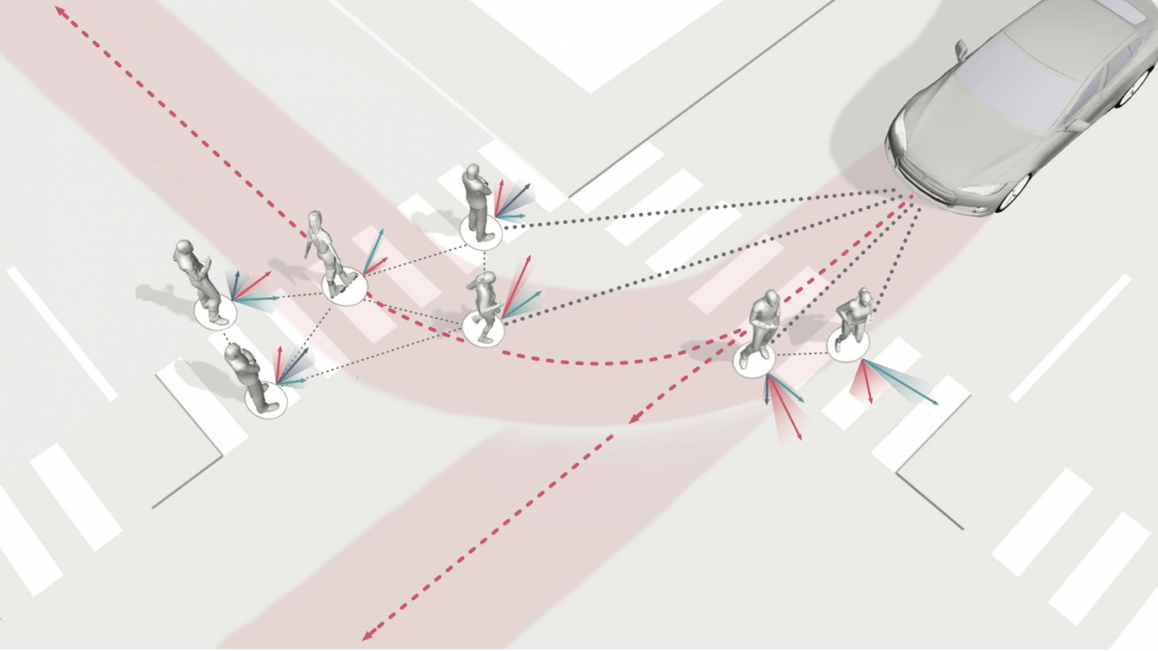
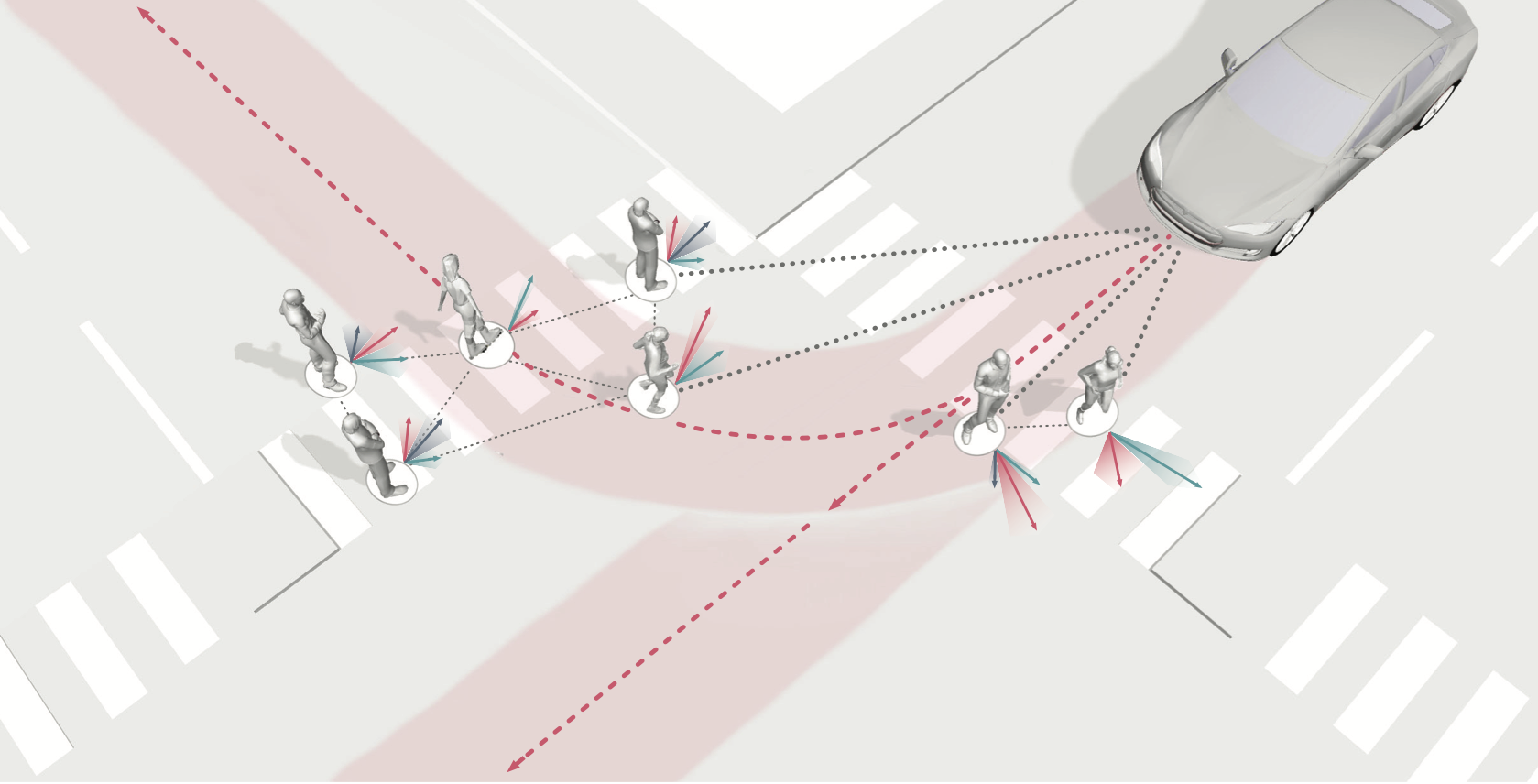
Merging into traffic is one of the most common day-to-day maneuvers we perform as drivers, yet still poses a major problem for self-driving vehicles. The reason that humans can naturally navigate through many social interaction scenarios, such as merging in traffic, is that they have an intrinsic capacity to reason about other people’s intents, beliefs, and desires, using such reasoning to predict what might happen in the future and make corresponding decisions1. However, many current autonomous systems do not use such proactive reasoning, which leads to difficulties when deployed in the real world. For example, there have been numerous instances of self-driving vehicles failing to merge into traffic, getting stuck in intersections, and making unnatural decisions that confuse others. As a result, imbuing autonomous systems with the ability to reason about other agents’ actions could enable more informed decision making and proactive actions to be taken in the presence of other intelligent agents, e.g., in human-robot interaction scenarios. Indeed, the ability to predict other agents’ behaviors (also known as multi-agent behavior prediction) has already become a core component of modern robotic systems. This holds especially true in safety-critical applications such as autonomous vehicles, which are currently being tested in the real world and targeting widespread deployment in the near future2. The diagram below illustrates a scenario where predicting the motion of other agents may help inform an autonomous vehicle’s path planning and decision making. Here, an autonomous vehicle is deciding whether to stay put or continue driving, depending on surrounding pedestrian movement. The red paths indicate future navigational plans for the vehicle, depending on its eventual destination.
At a high level, trajectory forecasting is the problem of predicting the path (trajectory) that some sentient agent (e.g., a bicyclist, pedestrian, car driver, or bus driver) will move along in the future given the trajectory that agent moved along in the past. In scenarios with multiple agents, we are also given their past trajectories, which can be used to infer how they interact with each other. Trajectories of length are usually represented as a sequence of positional waypoints (e.g., GPS coordinates). Since we aim to make good predictions, we evaluate methods by some metric that compares the predicted trajectory against the actual trajectory the agent takes (denoted earlier as ).
In this post, we will dive into methods for trajectory forecasting, building a taxonomy along the way that organizes approaches by their methodological choices and output structures. We will discuss common evaluation schemes, present new ones, and suggest ways to compare otherwise disparate approaches. Finally, we will highlight shortcomings in existing methods that complicate their integration in downstream robotic use cases. Towards this end, we will present a new approach for trajectory forecasting that addresses these shortcomings, achieves state-of-the-art experimental performance, and enables new avenues of deployment on real-world autonomous systems.
1. Methods for Multi-Agent Trajectory Forecasting
There are many approaches for multi-agent trajectory forecasting, ranging from classical, physics-based models to deterministic regressors to generative probabilistic models3. To explore them in a structured manner, we will first group methods by the assumptions they make followed by the technical approaches they employ, building a taxonomy of trajectory forecasting methodologies along the way.
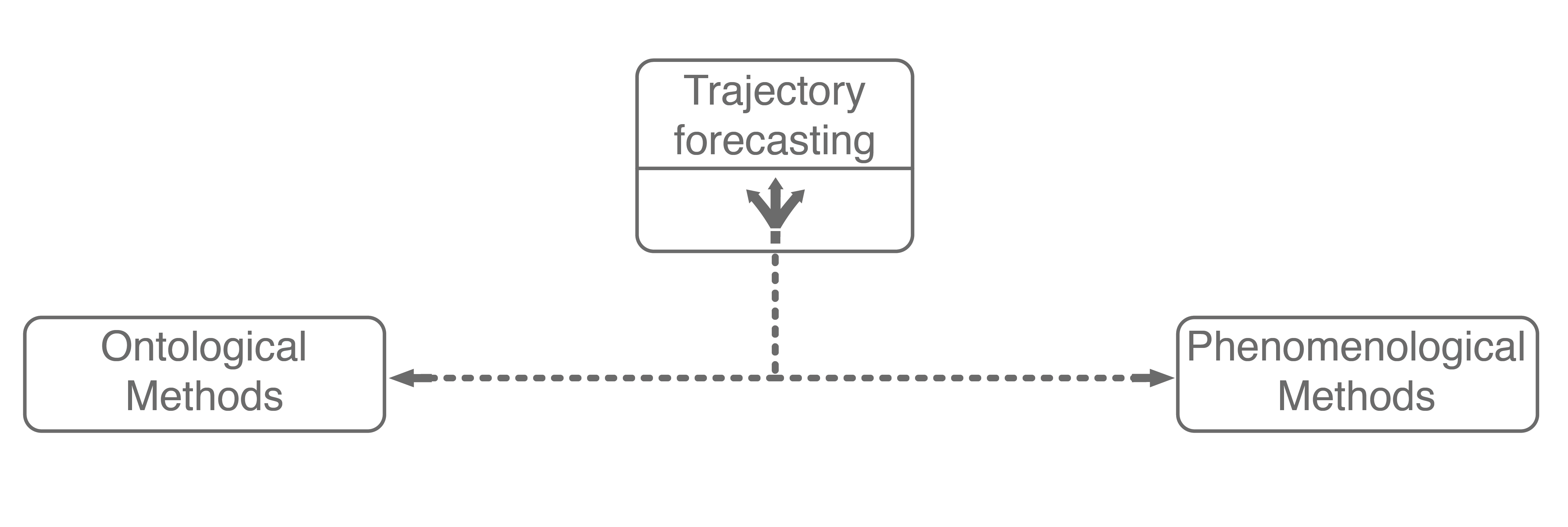
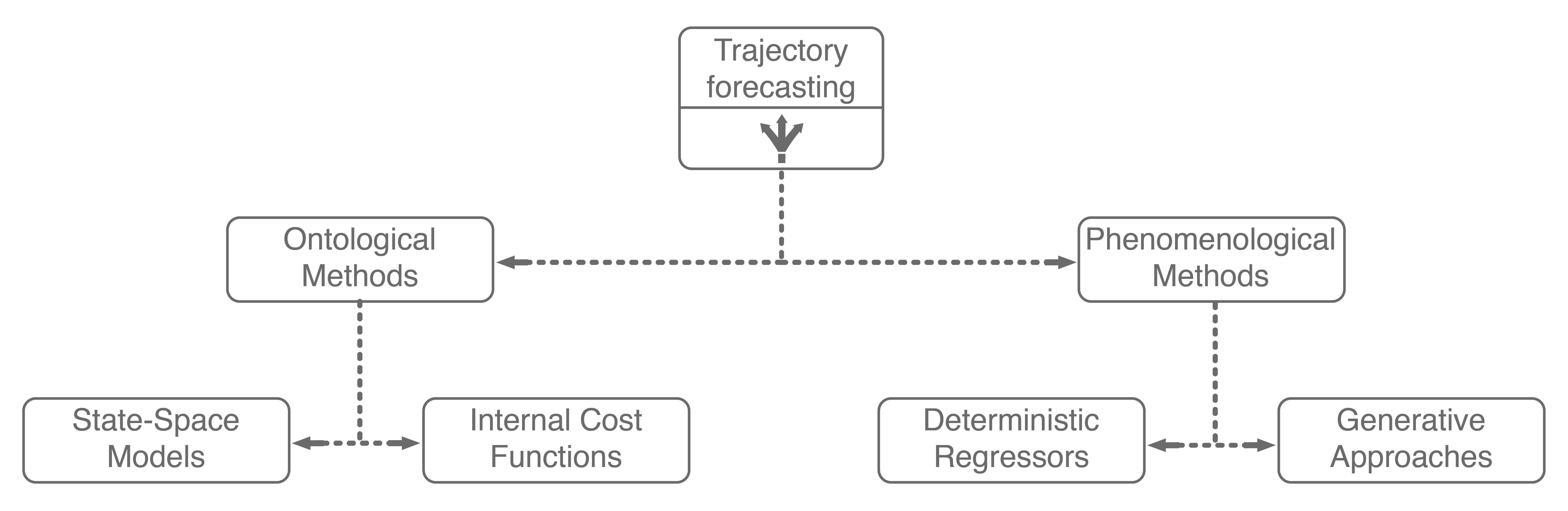
The first major assumption that approaches make is about the structure, if any, the problem possesses. In trajectory forecasting, this is manifested by approaches being either ontological or phenomenological. Ontological approaches (sometimes referred to as theory of mind) generally postulate (assume) some structure about the problem, whether that be a set of rules that agents follow or rough formulations of agents’ internal decision-making schemes. Phenomenological approaches do not make such assumptions, instead relying on a wealth of data to gleam agent behaviors without reasoning about underlying motivations.
1.1. Ontological Approaches
One of the simplest (and sometimes most effective) approaches for trajectory forecasting is classical mechanics. Usually, one assumes that they have a model that can predict the agent’s future state (also known as a dynamics model). With a dynamics model, one can predict the state (e.g., position, velocity, acceleration) of the agent several timesteps into the future. Such a simple approach is remarkably powerful, sometimes outperforming state-of-the-art approaches on real-world pedestrian modeling tasks4. However, pure dynamics integration alone does not account for the topology of the environment or interactions among agents, both of which are dominant effects. There have since been many approaches that mathematically formulate and model these interactions, exemplary methods include the intelligent driver model, MOBIL model, and Social Forces model.
More recently, inverse reinforcement learning (IRL) has emerged as a major ontological approach for trajectory forecasting. Given a set of agent trajectories in a scene , IRL attempts to learn the behavior and motivations of the agents. In particular, IRL formulates the motivation of an agent (e.g., crossing a sidewalk or turning right) with a mathematical formula, referred to as the reward function, shown below.
where refers to the reward value at a specific state (e.g., position, velocity, acceleration), is a set of weights to be learned, and is a set of extracted features that characterize the state . Thus, the IRL problem is to find the best weights . The main idea here is that solving a reinforcement learning problem with a successfully-learned reward function would yield a policy that matches , the original agent trajectories.
Unfortunately, there can be many such reward functions under which the original demonstrations are recovered. Thus, we need a way to choose between possible reward functions. A very popular choice is to pick the reward function with maximum entropy. This follows the principle of maximum entropy, which states that the most appropriate distribution to model a given set of data is the one with highest entropy among all feasible possibilities5. A reason why one would want to do this is that maximizing entropy minimizes the amount of prior information built into the model; there is less risk of overfitting to a specific dataset. This is named Maximum Entropy (MaxEnt) IRL, and has seen widespread use in modeling real-world navigation and driving behaviors.
To encode this maximum entropy choice into the IRL formulation from above, trajectories with higher rewards are valued exponentially more. Formally,
This distribution over paths also gives us a policy which can be sampled from. Specifically, the probability of an action is weighted by the expected exponentiated rewards of all trajectories that begin with that action.
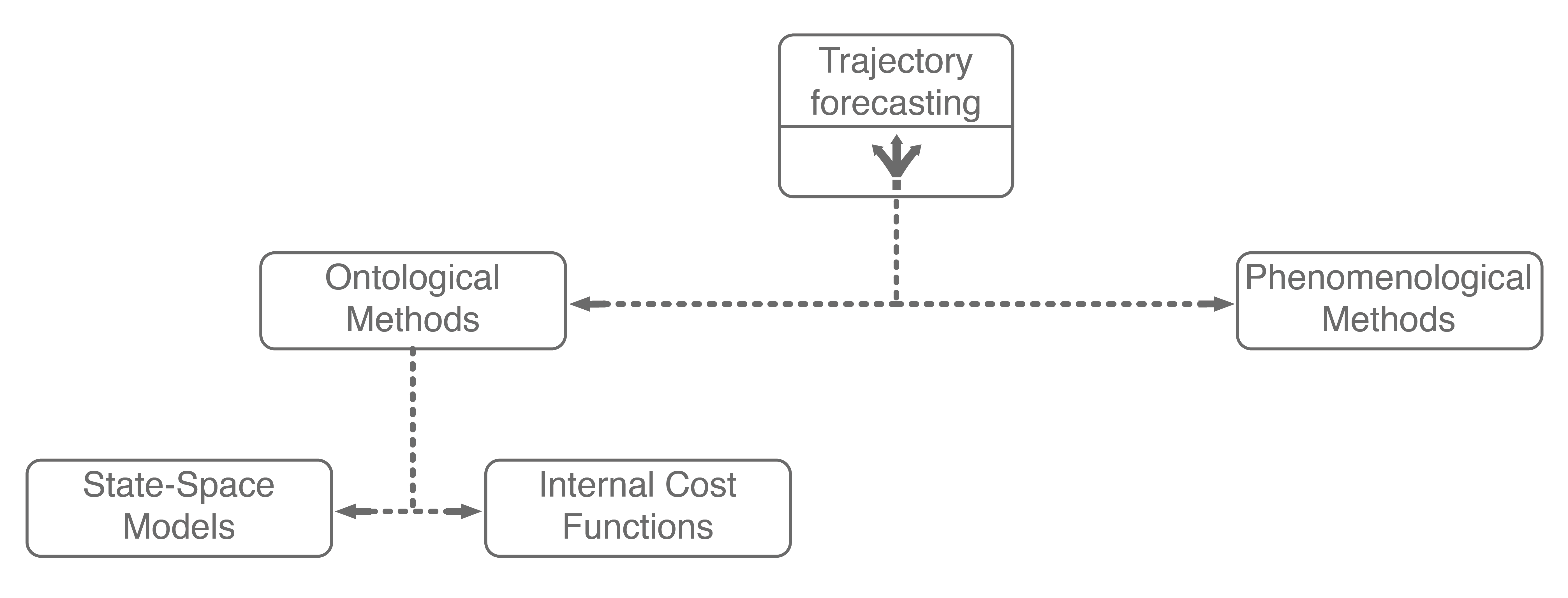
Wrapping up, ontological approaches provide a structured method for learning how sentient agents make decisions. Due to their strong structural assumptions, they are both very sample-efficient (there are not many parameters to learn), computationally-efficient to optimize, and generally easier to pair with decision making systems (e.g., game theory). However, these strong structural assumptions also limit the maximum performance that an ontological approach may achieve. For example, what if the expert’s actual reward function was non-linear, had different terms than the assumed reward function, or was non-Markovian (i.e., had a history dependency)? In these cases, the assumed model would necessarily underfit the observed data. Further, data availability is growing at an exponential rate, with terabytes of autonomous driving data publicly being released every few months (companies have access to orders of magnitude more internally). With so much data, it becomes natural to consider phenomenological approaches6, which form the other main branch of our trajectory forecasting taxonomy.
Including these two ontological approaches in our trajectory forecasting taxonomy yields the above tree. Next, we will dive into mainline phenomenological approaches.
1.2. Phenomenological Approaches
Phenomenological approaches are methods that make minimal assumptions about the structure of agents’ decision-making process. Instead, they rely on powerful general modeling techniques and a wealth of observation data to capture the kind of complexity encountered in environments with multiple interacting agents.
There have been a plethora of data-driven approaches for trajectory forecasting, mainly utilizing regressive methods such as Gaussian Process Regression (GPR)7 and deep learning, namely Long Short-Term Memory (LSTM) networks8 and Convolutional Neural Networks (CNNs)9, to good effect. Of these, LSTMs generally outperform GPR methods and are faster to evaluate online. As a result, they are commonly found as a core component of human trajectory models10. The reason why LSTMs perform well is that they are a purpose-built deep learning architecture for modeling temporal sequence data. Thus, practitioners usually model trajectory forecasting as a time series prediction problem and apply LSTM networks.
While these methods have enjoyed strong performance, there is a subtle point that limits their application to safety-critical problems such as autonomous driving: they only produce a single deterministic trajectory forecast. Safety-critical systems need to reason about many possible future outcomes, ideally with the likelihoods of each occurring, to make safe decisions online. As a result, methods that simultaneously forecast multiple possible future trajectories have been sought after recently.
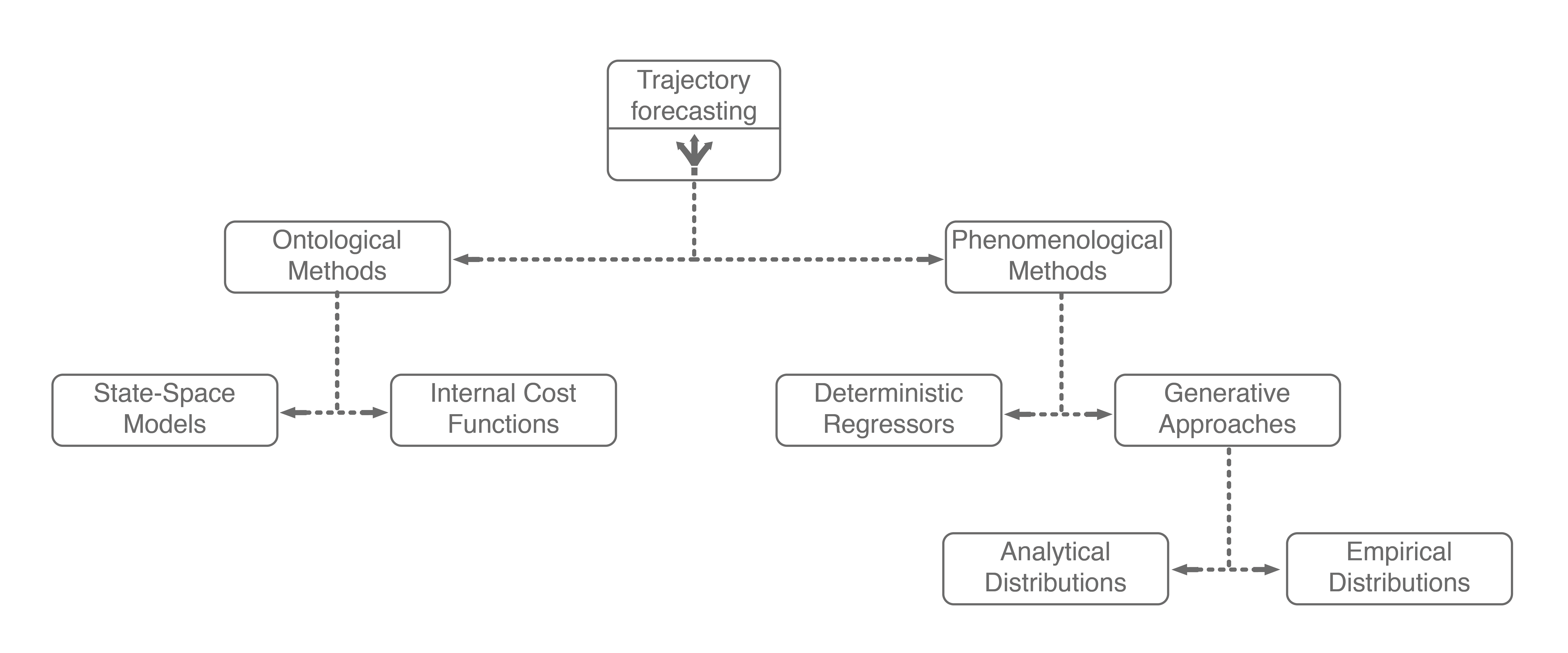
Generative approaches in particular have emerged as state-of-the-art trajectory forecasting methods due to recent advancements in deep generative models11. Notably, they have caused a paradigm shift from focusing on predicting the single best trajectory to producing a distribution of potential future trajectories. This is advantageous in autonomous systems as full distribution information is more useful for downstream tasks, e.g., motion planning and decision making, where information such as variance can be used to make safer decisions. Most works in this category use a deep recurrent backbone architecture (like an LSTM) with a latent variable model, such as a Conditional Variational Autoencoder (CVAE), to explicitly encode multimodality12, or a Generative Adversarial Network (GAN) to implicitly do so13. Common to both approach styles is the need to produce position distributions. GAN-based models can directly produce these and CVAE-based recurrent models usually rely on a bivariate Gaussian or bivariate Gaussian Mixture Model (GMM) to output position distributions. Including the two in our taxonomy balances out the right branch.
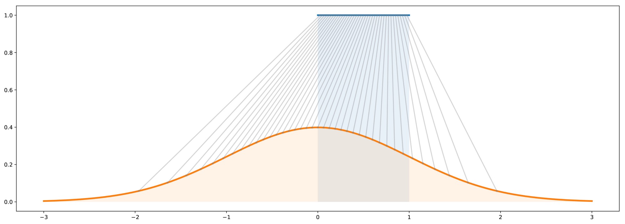
The main difference between GAN-based and CVAE-based approaches is in the form of their resulting output distribution. At a high level, GANs are generative models that generate data which, in aggregate, match the distribution of its training dataset . They achieve this by learning to map samples from a known distribution to samples of an unknown distribution for which we have samples, i.e., the training dataset. Intuitively, this is very similar to inverse transform sampling, which is a method for generating samples from any probability distribution given its cumulative distribution function. This is roughly illustrated below, where samples from a simple uniform distribution are mapped to a standard Gaussian distribution.
Thus, GANs can be viewed as learning an inverse transformation which maps a sample of a “simple” random variable to a sample of a “complex” random variable (conditioned on because that is the value being mapped to ). Thinking about this from the perspective of trajectory forecasting, is usually the trajectory history of the agent, information about neighboring agents, environmental information, etc. and is the trajectory forecast we are looking to output. Thus, it makes sense that one would want to produce predictions conditioned on past observations . However, this sampling-based structure also means that GANs can only produce empirical, and not analytical, distributions. Specifically, obtaining statistical properties like the mean and variance from a GAN can only be done approximately, through repeated sampling.
On the other hand, CVAEs tackle the problem of representing by decomposing it into subcomponents specified by the value of a latent variable . Formally,
Note that the sum in the above equation implies that is discrete (has finitely-many values). The latent variable can also be continuous, but there is work showing that discrete latent spaces lead to better performance (this also holds true for trajectory forecasting)14, so for this post we will only concern ourselves with a discrete . By decomposing in this way, one can produce an analytic output distribution. This is very similar to GMMs, which also decompose their desired distribution in this manner to produce an analytic distribution. This completes our taxonomy, and broadly summarizes current approaches for multi-agent trajectory forecasting.
With such a variety of approach styles, how do we know which is best? How can we determine if, for example, an approach that produces an analytic distribution outperforms a deterministic regressor?
2. Benchmarking Performance in Trajectory Forecasting
With such a broad range of approaches and output structures, it can be difficult to evaluate progress in the field. Even phrasing the question introduces biases towards methods. For example, asking the following excludes generative or probabilistic approaches: Given a trajectory forecast and the ground truth future trajectory , how does one evaluate how “close” the forecast is to the ground truth? We will start with this question, even if it is exclusionary for certain classes of methods.
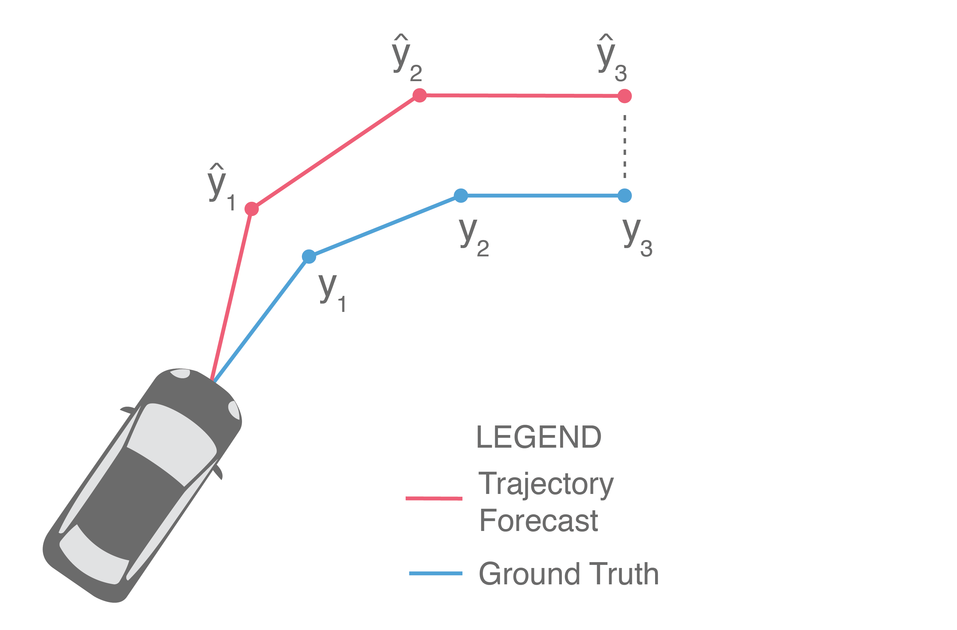
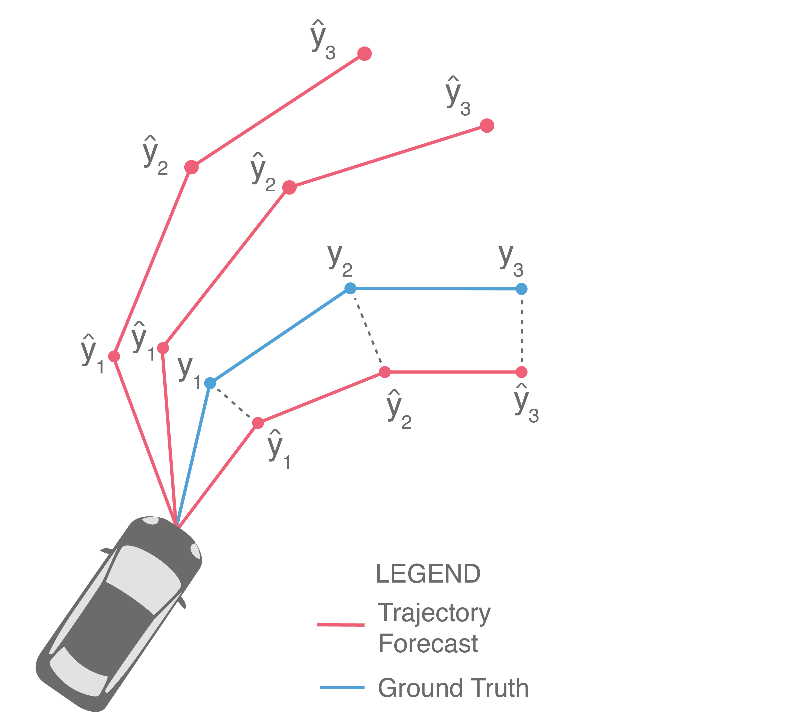
Illustrated above, one of the most common ways is to directly compare them side-by-side, i.e., measure how far is from for each and then average these distances to obtain the average error over the prediction horizon. This is commonly known as Average Displacement Error (ADE) and is usually reported in units of length, e.g., meters:
Often, we are also interested in the displacement error of only the final predicted point, illustrated below (in particular, only and are compared).
This provides a measure of a method’s error at the end of the prediction horizon, and is frequently referred to as Final Displacement Error (FDE). It is also usually reported in units of length.
ADE and FDE are the two main metrics used to evaluate deterministic regressors. While these metrics are natural for the task, easy to implement, and interpretable, they generally fall short in capturing the nuances of more sophisticated methods (see more on this below). It is for this reason, perhaps, that they have historically led to somewhat inconsistent reported results. For instance, there are contradictions between the results reported by the same authors in Gupta et al. (2018) and Alahi et al. (2016). Specifically, in Table 1 of Alahi et al. (2016), Social LSTM convincingly outperforms a baseline LSTM without pooling. However, in Table 1 of Gupta et al. (2018), Social LSTM is actually worse than the same baseline on average. Further, the values reported by Social Attention in Vemula et al. (2018) seem to have unusually high ratios of FDE to ADE. Nearly every other published method has FDE/ADE ratios around whereas Social Attention’s are around . Social Attention’s reported errors on the UCY – University dataset are especially striking, as its FDE after 12 timesteps is , which is its ADE of . This would make its prediction error on the other 11 timesteps essentially zero.
As mentioned earlier, safety-critical systems need to reason about many possible future outcomes, ideally with the likelihoods of each occurring, so that safe decision-making can take place which considers a whole range of possible futures. In this context, ADE and FDE are unsatisfactory because they focus on evaluating a single trajectory forecast. This leaves the following question: How do we evaluate generative approaches which produce many forecasts simultaneously, or even full distributions over forecasts?
Given the ground truth future trajectory and the ability to sample trajectory forecasts , how does one evaluate how “good” the samples are with respect to the ground truth? One initial idea, illustrated below, is to sample forecasts from the model and then return the performance of the best forecast. This is usually referred to as Best-of-N (BoN), along with the underlying performance metric used. For example, a Best-of-N ADE metric is illustrated below, since and we measure the ADE of the best forecast, i.e., the forecast with minimum ADE.
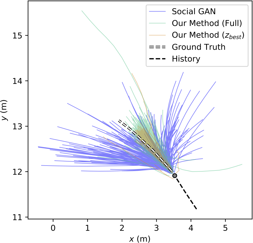
This is the main metric used by generative methods that produce empirical distributions, such as GAN-based approaches. The idea behind this evaluation scheme is to identify if the ground truth is near the forecasts produced by a few samples from the model ( is usually chosen to be small, e.g., ). Implicitly, this evaluation metric selects one sample as the best prediction and then evaluates it with the ADE/FDE metrics from before. However, this is inappropriate for autonomous driving because it requires knowledge of the future (in order to select the best prediction) and it is unclear how to relate BoN performance to the real world. It is also difficult to objectively compare methods using BoN because approaches that produce wildly different output samples may yield similar BoN metric values, as illustrated below.
This is a figure from our recent trajectory forecasting work at ICCV 2019 which compares versions of our method, the Trajectron, with that of the (generative, empirical) Social GAN. If one were to use a Best-of-N ADE or FDE metric on these outputs, both methods might perform similarly even though Social GAN produces outputs with significantly higher variance.
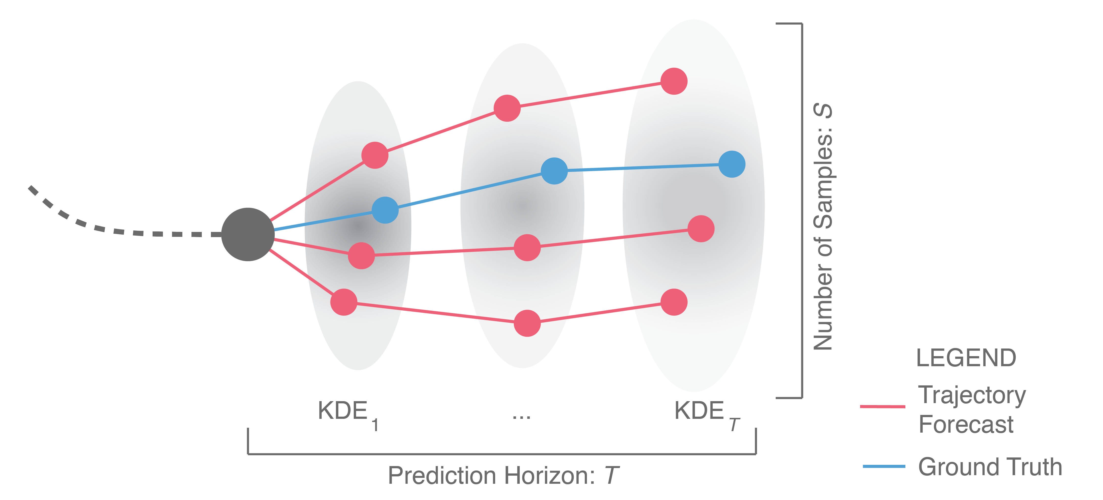
To address these shortcomings in the Best-of-N metric, we proposed a new evaluation scheme for generative, empirical methods in our recent ICCV 2019 paper15. Illustrated below, one starts by sampling many trajectories (, to obtain a representative set of outputs) from the methods being compared. A Kernel Density Estimate (KDE; a statistical tool that fits a probability density function to a set of samples) is then fit at each prediction timestep to obtain a probability density function (pdf) of the sampled positions at each timestep. From these pdfs, we compute the mean log-likelihood of the ground truth trajectory. This metric is called the KDE-based Negative Log-Likelihood (KDE NLL) and is reported in logarithmic units, i.e., nats.
KDE NLL does not suffer from the same downsides that BoN does, as (1) methods with wildly different outputs will yield wildly different KDEs, and (2) it does not require looking into the future during evaluation. Additionally, it fairly estimates a method’s NLL without any assumptions on the method’s output distribution structure; both empirical and analytical distributions can be sampled from. Thus, KDE NLL can be used to compare methods across taxonomy groups.
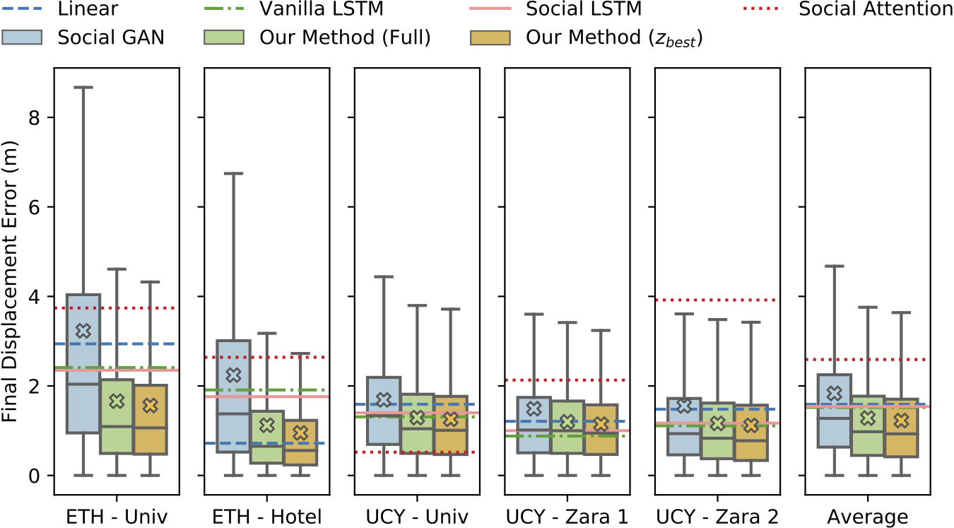
While KDE NLL can compare generative methods, deterministic lines of work are still disparate in their metrics and evaluating across the generative/deterministic boundary remains difficult. We also tried to tackle this in our 2019 ICCV paper, settling on the following comparison where we compared boxplots of generative methods alongside ADE and FDE (shown below) values from deterministic methods. The methods were trained and evaluated on the ETH and UCY pedestrian datasets, containing thousands of rich multi-human interaction scenarios.
Even though we created the above figure, it is not immediately obvious how to interpret it. Should one compare means and medians? Should one try statistical hypothesis tests between error distributions and mean error values from deterministic values? Unfortunately, using boxplots (as we did in our ICCV work) disregards the possibility for multimodal error distributions (i.e., a distribution with many peaks). Another possibility may be to let dataset curators decide the most relevant metrics for their dataset, e.g., the nuScenes dataset (a large-scale autonomous driving dataset from nuTonomy) has a prediction challenge with specific evaluation metrics. This may yield proper comparisons for a specific dataset, but it still allows for biases towards certain kinds of approaches and makes it difficult to compare approaches across datasets. For example, evaluating generative approaches with ADE and FDE ignores variance, which may make two different methods appear to perform the same (see trajectory samples from Trajectron vs. Social GAN in the earlier qualitative plot).
Overall, there is still much work to be done in standardizing metrics across approach styles and datasets. Some open questions in this direction are:
Do we really care equally about each waypoint in ADE? We know that forecasts degrade with prediction horizon, so why not focus on earlier or later prediction points more?
Why even aggregate displacement errors? We could compare the distribution of displacement errors per timestep, e.g., using a statistical hypothesis test like the t-test.
For methods that also produce variance information, why not weigh their predictions by ? This would enable methods to specify their own uncertainties and be rewarded, e.g., if they are making bad predictions in weird scenarios, but alerting that they are uncertain.
Since these forecasts are ultimately being used for decision making and control, a control-aware metric would be useful. For instance, we may want to evaluate an output’s control feasibility by how many control constraint violations there are on average over the course of a forecast.
We will now discuss our newly-released method for trajectory forecasting that addresses these cross-taxonomy evaluation quandaries by being explicitly designed to be simultaneously comparable with both generative and deterministic approaches. Further, this approach also addresses how to include system dynamics and additional data sources (e.g., maps, camera images, LiDAR point clouds) such that its forecasts are all physically-realizable by the modeled agent and consider the topology of the surrounding environment.
3. Trajectron++: Dynamically-Feasible Trajectory Forecasting With Heterogeneous Data
As mentioned earlier, nearly every trajectory forecasting method directly produces positions as their output. Unfortunately, this output structure makes it difficult to integrate with downstream planning and control modules, especially since purely-positional trajectory predictions do not respect dynamics constraints, e.g., the fact that a car cannot move sideways, which could lead to models producing trajectory forecasts that are unrealizable by the underlying control variables, e.g., predicting that a car will move sideways.
Towards this end, we have developed Trajectron++, a significant addition to the Trajectron framework, that addresses this shortcoming. In contrast to existing approaches, Trajectron++ explicitly accounts for system dynamics, and leverages heterogeneous input data (e.g., maps, camera images, LIDAR point clouds) to produce state-of-the-art trajectory forecasting results on a variety of large-scale real-world datasets and agent types.
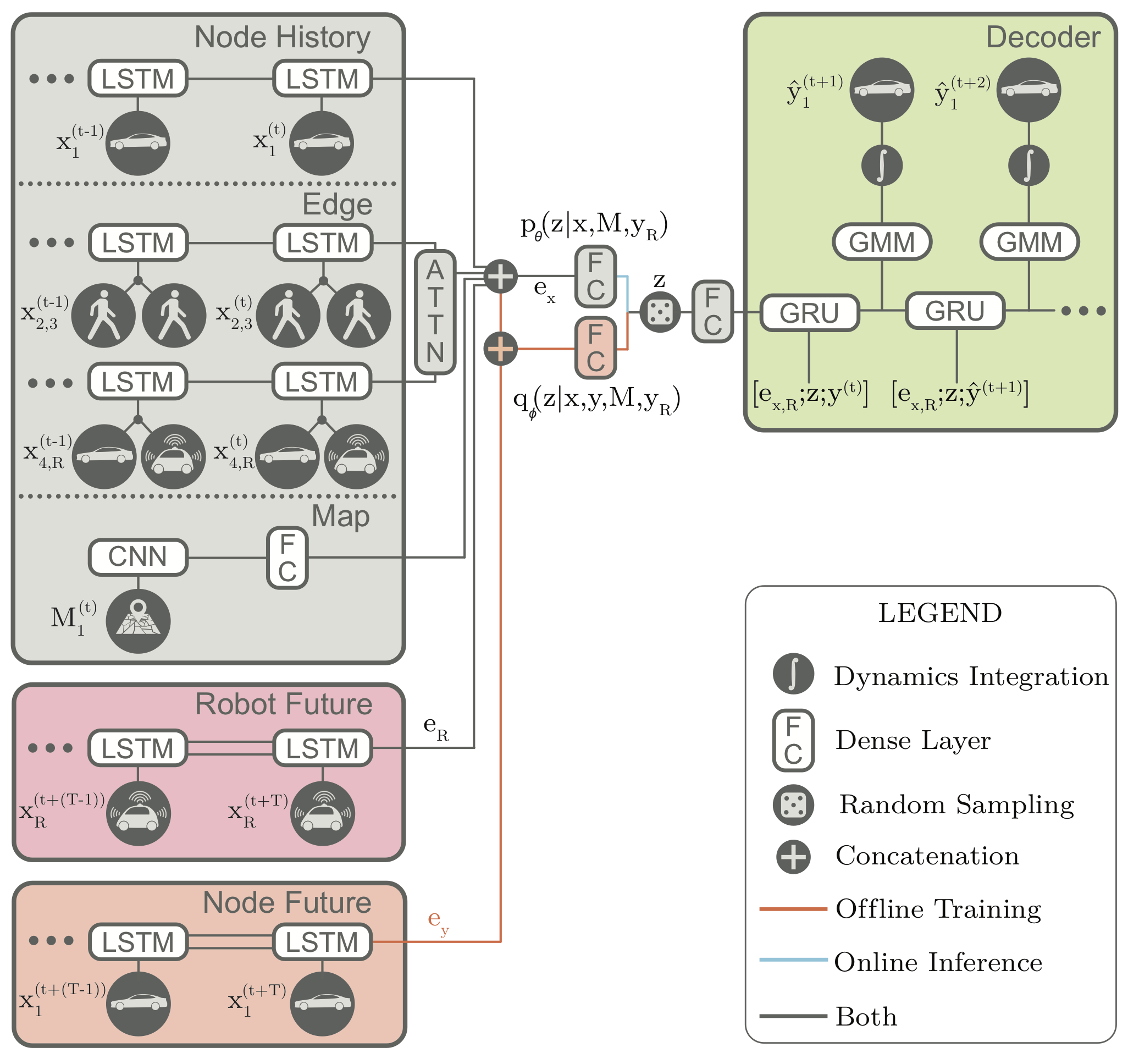
Trajectron++ is a graph-structured generative (CVAE-based) neural architecture that forecasts the trajectories of a general number of diverse agents while incorporating agent dynamics and heterogeneous data (e.g., semantic maps). It is designed to be tightly integrated with robotic planning and control frameworks; for example, it can produce predictions that are optionally conditioned on ego-agent motion plans. At a high level, it operates by first creating a spatiotemporal graph representation of a scene from its topology. Then, a similarly-structured deep learning architecture is generated that forecasts the evolution of node attributes, producing agent trajectories. An example of this is shown below.
A scene around the ego-vehicle in the nuScenes dataset is shown. From the distances between different agents (e.g., pedestrians, cars), a spatiotemporal graph is built (left) which then dictates how the corresponding neural network architecture (right) is constructed. The architecture models agents by encoding the agent’s history and local interactions (edges).
We will focus on two aspects of our model, each of which address one of the problems we previously highlighted (considering dynamics and comparing across the trajectory forecasting taxonomy).
3.1. Incorporating System Dynamics into Generative Trajectory Forecasting
One of the main contributions of Trajectron++ is presenting a method for producing dynamically-feasible output trajectories. Most CVAE-based generative methods capture fine-grained uncertainty in their outputs by producing the parameters of a bivariate Gaussian distribution (i.e., its mean and covariance) and then sampling position waypoints from it. However, this direct modeling of position is ignorant of an agent’ governing dynamics and relies on the neural network architecture to learn dynamics.
While neural networks can do this, we are already good at modeling the dynamics of many systems, including pedestrians (as single integrators) and vehicles (e.g., as dynamically-extended unicycles)16. Thus, Trajectron++ instead focuses on forecasting distributions of control sequences which are then integrated through the agent’s dynamics to produce positions. This ensures that the output trajectories are physically realizable as they have associated control strategies. Note that the full distribution itself is integrated through the dynamics. This can be done for each latent behavior mode via the Kalman Filter prediction equations (for linear dynamics models) or the Extended Kalman Filter prediction equations (for nonlinear dynamics models).
As a bonus, adding agent dynamics to the model yields noticeable performance improvements across all evaluation metrics. Broadly, this makes sense as the model’s loss function (the standard Evidence Lower Bound CVAE loss) can now be directly specified over the desired quantity (position) while still respecting dynamic constraints.
3.2. Leveraging Heterogeneous Data Sources
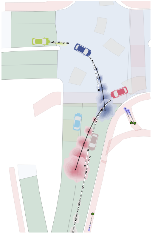
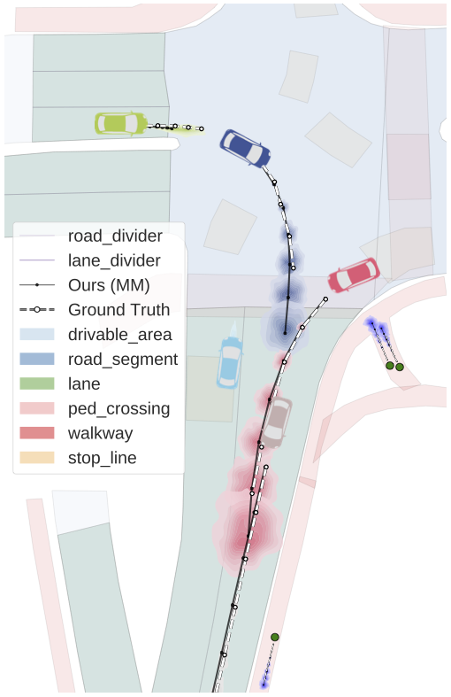
An additional feature of Trajectron++ is its ability to combine data from a variety of sources to produce forecasts. In particular, the presence of a single backbone representation vector, denoted in the above architecture diagram, enables for the seamless addition of new data via concatenation. To illustrate this, we show the benefits of including high-definition maps in the figure below. In it, we can see that the model is able to improve its predictions in turns, better reflecting the local lane geometry.
Left: Without map information, the model tends to undershoot turns. Right: Encoding a local map of the agent’s surroundings notably increases Trajectron++’s accuracy and confidence in turns. It is able to use semantic labels (shown in color) to reason about where agents can go.
3.3. Simultaneously Producing Both Generative and Deterministic Outputs
A key feature of the Trajectron and Trajectron++ models is their combination of a CVAE with a Gaussian output. Specifically, the “GMM” in the above architecture diagram only has one component, i.e., it is just a multivariate Gaussian. Thus, the model’s overall output is
which is the definition of a GMM! Thus, each component , which is meant to model high-level latent behaviors, ends up specifying a set of parameters for a Gaussian output distribution over control variables. With such a form, we can easily produce both generative and deterministic outputs. The following are the main four outputs that Trajectron++ can produce.
Most Likely (ML): This is the model’s deterministic and most-likely single output. The high-level latent behavior mode and output trajectory are the modes of their respective distributions, where
: Predictions from the model’s most-likely high-level latent behavior mode, where
Full: The model’s full sampled output, where and are sampled sequentially according to
Distribution: Due to the use of a discrete Categorical latent variable and Gaussian output structure, the model can provide an analytic output distribution by directly computing
Thus, to compare against deterministic methods we use Trajectron++’s most-likely prediction with ADE and FDE. To compare against generative empirical or analytical methods, we use any of , Full, or Distribution with KDE NLL. In summary, Trajectron++ can be directly compared to any method that produces either a single trajectory or a distribution thereof.
Trajectron++ serves as a first step along a broader research thrust to better integrate modern trajectory forecasting approaches with robotic planning, decision making, and control. In particular, we are broadening our focus from purely minimizing benchmark error to also considering the advancements needed to successfully deploy modern trajectory forecasting methods to the real world, where properties like runtime, scalability, and data dependence play increasingly important roles. This in turn raises further research questions, for example:
What output representation best suits downstream planners? Predicting positional information alone makes it difficult to use some planning, decision making, and control algorithms.
What is required of perception? How difficult is it to obtain the desired input information?
Some research groups are already tackling these types of questions17, viewing trajectory forecasting as a modular component that is integrated with perception, planning, and control modules.
4. Conclusion
Now that there is a large amount of publicly-available trajectory forecasting data, we have crossed the threshold where data-driven, phenomenological approaches generally surpass the performance of ontological methods. In particular, recent advances in deep generative modeling have brought forth a probabilistic paradigm shift in multi-agent trajectory forecasting, leading to new considerations about evaluation metrics and downstream use cases.
In this post, we constructed a taxonomy of existing mainline approaches (e.g., Social Forces and IRL) and newer research (e.g., GAN-based and CVAE-based approaches), discussed their evaluation schemes and suggested ways to compare approaches across taxonomy groups, and highlighted shortcomings that complicate their integration in downstream robotic use cases. Towards this end, we present Trajectron++, a novel phenomenological trajectory forecasting approach that incorporates dynamics knowledge and the capacity for heterogeneous data inclusion. As a step towards the broader research thrust of integrating trajectory forecasting with autonomous systems, Trajectron++ produces dynamically-feasible trajectories in a wide variety of output formats depending on the specific downstream use case. It achieves state-of-the-art performance on both generative and deterministic benchmarks, and enables new avenues of deployment on real-world autonomous systems.
There are still many open questions, especially in terms of standard evaluation metrics, model interpretability, and broader architectural considerations stemming from future integration with downstream planning and control algorithms. This especially rings true now that deep learning approaches have outweighed others in popularity and performance, and are targeting deployment on real-world safety-critical robotic systems.
All of our code, models, and data are available here. If you have any questions, please contact Boris Ivanovic.
Acknowledgements
Many thanks to Karen Leung and Marco Pavone for comments and edits on this blog post, Matteo Zallio for visually communicating our ideas, and Andrei Ivanovic for proofreading.
Gweon and Saxe provide a good overview of this concept, commonly known as “theory of mind”, in this book chapter. ↩
For example, both Uber and Waymo provide safety reports discussing what they have learned from real-world testing as well as their strategies for developing safe self-driving vehicles that can soon operate among humans. ↩
Posted by Philip Quinn and Wenxin Feng, Research Scientists, Android UX
Touch input has traditionally focussed on two-dimensional finger pointing. Beyond tapping and swiping gestures, long pressing has been the main alternative path for interaction. However, a long press is sensed with a time-based threshold where a user’s finger must remain stationary for 400–500 ms. By its nature, a time-based threshold has negative effects for usability and discoverability as the lack of immediate feedback disconnects the user’s action from the system’s response. Fortunately, fingers are dynamic input devices that can express more than just location: when a user touches a surface, their finger can also express some level of force, which can be used as an alternative to a time-based threshold.
While a variety of force-based interactions have been pursued, sensing touch force requires dedicated hardware sensors that are expensive to design and integrate. Further, research indicates that touch force is difficult for people to control, and so most practical force-based interactions focus on discrete levels of force (e.g., a soft vs. firm touch) — which do not require the full capabilities of a hardware force sensor.
For a recent update to the Pixel 4, we developed a method for sensing force gestures that allowed us to deliver a more expressive touch interaction experience By studying how the human finger interacts with touch sensors, we designed the experience to complement and support the long-press interactions that apps already have, but with a more natural gesture. In this post we describe the core principles of touch sensing and finger interaction, how we designed a machine learning algorithm to recognise press gestures from touch sensor data, and how we integrated it into the user experience for Pixel devices.
Touch Sensor Technology and Finger Biomechanics A capacitive touch sensor is constructed from two conductive electrodes (a drive electrode and a sense electrode) that are separated by a non-conductive dielectric (e.g., glass). The two electrodes form a tiny capacitor (a cell) that can hold some charge. When a finger (or another conductive object) approaches this cell, it ‘steals’ some of the charge, which can be measured as a drop in capacitance. Importantly, the finger doesn’t have to come into contact with the electrodes (which are protected under another layer of glass) as the amount of charge stolen is inversely proportional to the distance between the finger and the electrodes.
Left: A finger interacts with a touch sensor cell by ‘stealing’ charge from the projected field around two electrodes. Right: A capacitive touch sensor is constructed from rows and columns of electrodes, separated by a dielectric. The electrodes overlap at cells, where capacitance is measured.
The cells are arranged as a matrix over the display of a device, but with a much lower density than the display pixels. For instance, the Pixel 4 has a 2280 × 1080 pixel display, but a 32 × 15 cell touch sensor. When scanned at a high resolution (at least 120 Hz), readings from these cells form a video of the finger’s interaction.
Slowed touch sensor recordings of a user tapping (left), pressing (middle), and scrolling (right).
Capacitive touch sensors don’t respond to changes in force per se, but are tuned to be highly sensitive to changes in distance within a couple of millimeters above the display. That is, a finger contact on the display glass should saturate the sensor near its centre, but will retain a high dynamic range around the perimeter of the finger’s contact (where the finger curls up).
When a user’s finger presses against a surface, its soft tissue deforms and spreads out. The nature of this spread depends on the size and shape of the user’s finger, and its angle to the screen. At a high level, we can observe a couple of key features in this spread (shown in the figures): it is asymmetric around the initial contact point, and the overall centre of mass shifts along the axis of the finger. This is also a dynamic change that occurs over some period of time, which differentiates it from contacts that have a long duration or a large area.
Touch sensor signals are saturated around the centre of the finger’s contact, but fall off at the edges. This allows us to sense small deformations in the finger’s contact shape caused by changes in the finger’s force.
However, the differences between users (and fingers) makes it difficult to encode these observations with heuristic rules. We therefore designed a machine learning solution that would allow us to learn these features and their variances directly from user interaction samples.
Machine Learning for Touch Interaction We approached the analysis of these touch signals as a gesture classification problem. That is, rather than trying to predict an abstract parameter, such as force or contact spread, we wanted to sense a press gesture — as if engaging a button or a switch. This allowed us to connect the classification to a well-defined user experience, and allowed users to perform the gesture during training at a comfortable force and posture.
Any classification model we designed had to operate within users’ high expectations for touch experiences. In particular, touch interaction is extremely latency-sensitive and demands real-time feedback. Users expect applications to be responsive to their finger movements as they make them, and application developers expect the system to deliver timely information about the gestures a user is performing. This means that classification of a press gesture needs to occur in real-time, and be able to trigger an interaction at the moment the finger’s force reaches its apex.
We therefore designed a neural network that combined convolutional (CNN) and recurrent (RNN) components. The CNN could attend to the spatial features we observed in the signal, while the RNN could attend to their temporal development. The RNN also helps provide a consistent runtime experience: each frame is processed by the network as it is received from the touch sensor, and the RNN state vectors are preserved between frames (rather than processing them in batches). The network was intentionally kept simple to minimise on-device inference costs when running concurrently with other applications (taking approximately 50 µs of processing per frame and less than 1 MB of memory using TensorFlow Lite).
An overview of the classification model’s architecture.
The model was trained on a dataset of press gestures and other common touch interactions (tapping, scrolling, dragging, and long-pressing without force). As the model would be evaluated after each frame, we designed a loss function that temporally shaped the label probability distribution of each sample, and applied a time-increasing weight to errors. This ensured that the output probabilities were temporally smooth and converged towards the correct gesture classification.
User Experience Integration Our UX research found that it was hard for users to discover force-based interactions, and that users frequently confused a force press with a long press because of the difficulty in coordinating the amount of force they were applying with the duration of their contact. Rather than creating a new interaction modality based on force, we therefore focussed on improving the user experience of long press interactions by accelerating them with force in a unified press gesture. A press gesture has the same outcome as a long press gesture, whose time threshold remains effective, but provides a stronger connection between the outcome and the user’s action when force is used.
A user long pressing (left) and firmly pressing (right) on a launcher icon.
This also means that users can take advantage of this gesture without developers needing to update their apps. Applications that use Android’s GestureDetector or View APIs will automatically get these press signals through their existing long-press handlers. Developers that implement custom long-press detection logic can receive these press signals through the MotionEvent classification API introduced in Android Q.
Through this integration of machine-learning algorithms and careful interaction design, we were able to deliver a more expressive touch experience for Pixel users. We plan to continue researching and developing these capabilities to refine the touch experience on Pixel, and explore new forms of touch interaction.
Acknowledgements This project is a collaborative effort between the Android UX, Pixel software, and Android framework teams.
Amazon scientists are on the cutting edge of using math-based logic to provide better network security, access management, and greater reliability.Read More
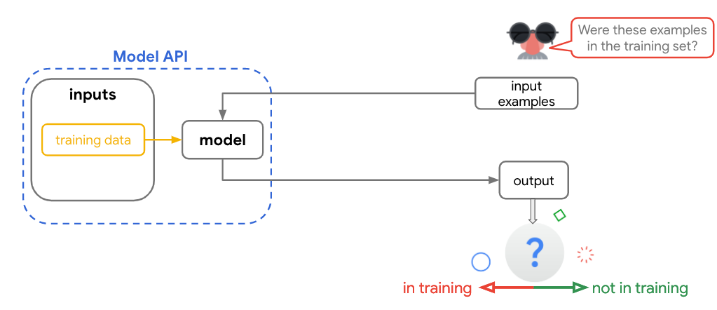
Overview of a membership inference attack. An attacker tries to figure out whether certain examples were part of the training data.
Today, we’re excited to announce a new experimental module in TensorFlow Privacy (GitHub) that allows developers to assess the privacy properties of their classification models.
Privacy is an emerging topic in the Machine Learning community. There aren’t canonical guidelines to produce a private model. There is a growing body of research showing that a machine learning model can leak sensitive information of the training dataset, thus creating a privacy risk for users in the training set.
Last year, we launched TensorFlow Privacy, enabling developers to train their models with differential privacy. Differential privacy adds noise to hide individual examples in the training dataset. However, this noise is designed for academic worst-case scenarios and can significantly affect model accuracy.
These challenges led us to tackle privacy from a different perspective. A few years ago, research around the privacy properties of machine learning models started to emerge. Cost-efficient “membership inference attacks” predict whether a specific piece of data was used during training. If an attacker is able to make a prediction with high accuracy, they will likely succeed in figuring out if a data piece was used in the training set. The biggest advantage of a membership inference attack is that it is easy to perform, i.e., does not require any re-training.
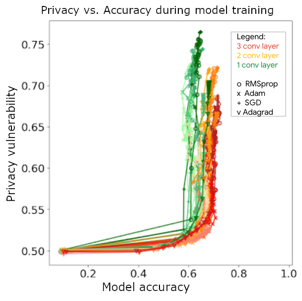
A test produces a vulnerability score that determines whether the model leaks information from the training set. We found that this vulnerability score often decreases with heuristics, such as early stopping or using DP-SGD for training.
Membership inference attack on models for CIFAR10. The x-axis is the test accuracy of the model, and y-axis is vulnerability score (lower means more private). Vulnerability grows while test accuracy remains the same – better generalization could prevent privacy leakage.
Unsurprisingly, differential privacy helps in reducing these vulnerability scores. Even with very small amounts of noise, the vulnerability score decreased.
After using membership inference tests internally, we’re sharing them with developers to help them build more private models, explore better architecture choices, use regularization techniques such as early stopping, dropout, weight decay, and input augmentation, or collect more data. Ultimately, these tests can help the developer community identify more architectures that incorporate privacy design principles and data processing choices.
We hope this library will be the starting point of a robust privacy testing suite that can be used by any machine learning developer around the world. Moving forward, we’ll explore the feasibility of extending membership inference attacks beyond classifiers and develop new tests. We’ll also explore adding this test to the TensorFlow ecosystem by integrating with TFX.
Reach out to tf-privacy@google.com and let us know how you’re using this new module. We’re keen on hearing your stories, feedback, and suggestions!
Acknowledgments: Yurii Sushko, Andreas Terzis, Miguel Guevara, Niki Kilbertus, Vadym Doroshenko, Borja De Balle Pigem, Ananth Raghunathan. Read More
We propose a benchmark called RL Unplugged to evaluate and compare offline RL methods. RL Unplugged includes data from a diverse range of domains including games (e.g., Atari benchmark) and simulated motor control problems (e.g. DM Control Suite). The datasets include domains that are partially or fully observable, use continuous or discrete actions, and have stochastic vs. deterministic dynamics.Read More


 Drew Meyer is a Product Marketing Manager at Alexa. He helps developers understand the latest in AI and ML capabilities for voice so they can build exciting new experiences with Alexa. In his spare time he plays with his twin boys, mountain bikes, and plays guitar.
 Vikas Shah is an Enterprise Solutions Architect at Amazon web services. He is a technology enthusiast who enjoys helping customers find innovative solutions to complex business challenges. His areas of interest are ML, IoT, robotics and storage. In his spare time, Vikas enjoys building robots, hiking, and traveling.