Building AI-powered forecasting automation with Amazon Forecast by applying MLOps

Building AI-powered forecasting automation with Amazon Forecast by applying MLOps

This post demonstrates how to create a serverless Machine Learning Operations (MLOps) pipeline to develop and visualize a forecasting model built with Amazon Forecast. Because Machine Learning (ML) workloads need to scale, it’s important to break down the silos among different stakeholders to capture business value. The MLOps model makes sure that the data science, production, and operations teams work together seamlessly across workflows that are as automated as possible, ensuring smooth deployments and effective ongoing monitoring.

Similar to the DevOps model in software development, the MLOps model in ML helps build code and integration across ML tools and frameworks. You can automate, operationalize, and monitor data pipelines without having to rewrite custom code or rethink existing infrastructures. MLOps helps scale existing distributed storage and processing infrastructures to deploy and manage ML models at scale. It can also be implemented to track and visualize drift over time for all models across the organization in one central location and implement automatic data validation policies.

MLOps combines best practices from DevOps and the ML world by applying continuous integration, continuous deployment, and continuous training. MLOps helps streamline the lifecycle of ML solutions in production. For more information, see the whitepaper Machine Learning Lens: AWS Well-Architected Framework.

In the following sections you will build, train, and deploy a time-series forecasting model leveraging an MLOps pipeline encompassing Amazon Forecast, AWS Lambda, and AWS Step Functions. To visualize the generated forecast, you will use a combination of AWS serverless analytics services such as Amazon Athena and Amazon QuickSight.

Solution architecture

In this section, you deploy an MLOps architecture that you can use as a blueprint to automate your Amazon Forecast usage and deployments. The provided architecture and sample code help you build an MLOps pipeline for your time series data, enabling you to generate forecasts to define future business strategies and fulfil customer needs.

You can build this serverless architecture using AWS-managed services, which means you don’t need to worry about infrastructure management while creating your ML pipeline. This helps iterate through a new dataset and adjust your model by tuning features and hyperparameters to optimize performance.

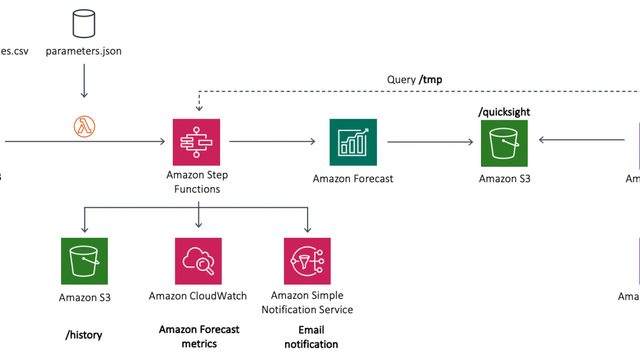
The following diagram illustrates the components you will build throughout this post.

In the preceding diagram, the serverless MLOps pipeline is deployed using a Step Functions workflow, in which Lambda functions are stitched together to orchestrate the steps required to set up Amazon Forecast and export the results to Amazon Simple Storage Service (Amazon S3).

The architecture contains the following components:

  • The time series dataset is uploaded to the Amazon S3 cloud storage under the /train directory (prefix).
  • The uploaded file triggers Lambda, which initiates the MLOps pipeline built using a Step Functions state machine.
  • The state machine stitches together a series of Lambda functions to build, train, and deploy a ML model in Amazon Forecast. You will learn more details about the state machine’s Lambda components in the next section.
  • For log analysis, the state machine uses Amazon CloudWatch, which captures Forecast metrics. You use Amazon Simple Notification Service (Amazon SNS) to send email notifications when the final forecasts become available in the source Amazon S3 bucket in the /forecast directory. The ML pipeline saves any old forecasts in the /history directory.
  • Finally, you will use Athena and QuickSight to provide a visual presentation of the current forecast.

In this post, you use the Individual household electric power consumption dataset available in the UCI Machine Learning Repository. The time series dataset aggregates hourly energy consumption for various customers households and shows spikes in energy utilization over weekdays. You can replace the sample data as needed for later use cases.

Now that you are familiar with the architecture, you’re ready to explore the details of each Lambda component in the state machine.

Building an MLOps pipeline using Step Functions

In the previous section, you learned that the Step Functions state machine is the core of the architecture automating the entire MLOps pipeline. The following diagram illustrates the workflow deployed using the state machine.

As shown in preceding diagram, the Lambda functions from the Step Functions workflow are as follows (the steps also highlight the mapping between Lambda functions and the parameters used from the params.json file stored in Amazon S3):

  • Create-Dataset – Creates a Forecast dataset. The information about the dataset helps Forecast understand how to consume the data for model training.
  • Create-DatasetGroup – Creates a dataset group.
  • Import-Data – Imports your data into a dataset that resides inside a dataset group.
  • Create-Predictor – Creates a predictor with a forecast horizon that the parameters file specifies.
  • Create-Forecast – Creates the forecast and starts an export job to Amazon S3, including quantiles specified in the parameters file.
  • Update-Resources – Creates the necessary Athena resources and transforms the exported forecasts to the same format as the input dataset.
  • Notify Success – Sends an email alerting when the job is finished by posting a message to Amazon SNS.
  • Strategy-Choice – Checks whether to delete the Forecast resources, according to the parameters file.
  • Delete-Forecast – Deletes the forecast and keeps the exported data.
  • Delete-Predictor – Deletes the predictor.
  • Delete-ImportJob – Deletes the Import-Data job in Forecast.

In Amazon Forecast, a dataset group is an abstraction that contains all the datasets for a particular collection of forecasts. There is no information sharing between dataset groups; to try out various alternatives to the schemas, you create a new dataset group and make changes inside its corresponding datasets. For more information, see Datasets and Dataset Groups. For this use case, the workflow imports a target time series dataset into a dataset group.

After completing these steps, the workflow triggers the predictor training job. A predictor is a Forecast-trained model used for making forecasts based on time series data. For more information, see Predictors.

When your predictor is trained, the workflow triggers the creation of a forecast using that predictor. During forecast creation, Amazon Forecast trains a model on the entire dataset before hosting the model and making inferences. For more information, see Forecasts.

The state machine sends a notification email to the address specified at the deployment of a successful forecast export. After exporting your forecast, the Update-Resources step reformats the exported data so Athena and QuickSight can easily consume it.

You can reuse this MLOps pipeline to build, train, and deploy other ML models by replacing the algorithms and datasets in the Lambda function for each step.

Prerequisites

Before you deploy the architecture, complete the following prerequisite steps:

  1. Install Git.
  2. Install the AWS Serverless Application Model (AWS SAM) CLI on your system. For instructions, see Installing the AWS SAM CLI. Make sure the latest version is installed with the following code:
    sam --version 

Deploying the sample architecture to your AWS account

To simplify deployment, this post provides the entire architecture as infrastructure as code using AWS CloudFormation and is available in the Forecast Visualization Automation Blogpost GitHub repo. You use AWS SAM to deploy this solution.

  1. Clone the Git repo. See the following code:
    git clone https://github.com/aws-samples/amazon-forecast-samples.git

    The code is also available on the Forecast Visualization Automation Blogpost GitHub repo.

  2. Navigate to the newly created amazon-forecast-samples/ml_ops/visualization_blog directory and enter the following code to start solution deployment:
    cd amazon-forecast-samples/ml_ops/visualization_blog
    
    sam build && sam deploy --guided
    

    At this stage, AWS SAM builds a CloudFormation template change set. After a few seconds, AWS SAM prompts you to deploy the CloudFormation stack.

  3. Provide parameters for the stack deployment. This post uses the following parameters; you can keep the default parameters:
    Setting default arguments for 'sam deploy'
    	=========================================
    	Stack Name [ForecastSteps]:  <Enter Stack Name e.g.  - forecast-blog-stack>
    	AWS Region [us-east-1]: <Enter region e.g. us-east-1>
    	Parameter Email [youremail@yourprovider.com]: <Enter valid e-mail id>
    	Parameter ParameterFile [params.json]: <Leave Default>
    	#Shows you resources changes to be deployed and require a 'Y' to initiate deploy
    	Confirm changes before deploy [Y/n]: y
    	#SAM needs permission to be able to create roles to connect to the resources in   
            your template
    	Allow SAM CLI IAM role creation [Y/n]: y
            Save arguments to samconfig.toml [Y/n]: n 
    

    AWS SAM creates an AWS CloudFormation change set and asks for confirmation.

  4. Enter Y.

For more information about change sets, see Updating Stacks Using Change Sets.

After a successful deployment, you see the following output:

CloudFormation outputs from the deployed stack
------------------------------------------------------------
Outputs                                                                                                                                
-------------------------------------------------------------
Key                 AthenaBucketName                                                                                                   
Description         Athena bucket name to drop your files                                                                              
Value               forecast-blog-stack-athenabucket-1v6qnz7n5f13w                                                                     

Key                 StepFunctionsName                                                                                                  
Description         Step Functions Name                                                                                                
Value               arn:aws:states:us-east-1:789211807855:stateMachine:DeployStateMachine-5qfVJ1kycEOj                                 

Key                 ForecastBucketName                                                                                                 
Description         Forecast bucket name to drop your files                                                                            
Value               forecast-blog-stack-forecastbucket-v61qpov2cy8c                                                                    
-------------------------------------------------------------
Successfully created/updated stack - forecast-blog-stack in us-east-1
  1. On the AWS CloudFormation console, on the Outputs tab, record the value of ForecastBucketName, which you use in the testing step.

Testing the sample architecture

The following steps outline how to test the sample architecture. To trigger the Step Functions workflow, you need to upload two files to the newly created S3 bucket: a parameter file and the time series training dataset.

  1. Under the same directory in which you cloned the GitHub repo, enter the following code, replacing YOURBUCKETNAME with the value from the AWS CloudFormation Outputs tab that you copied earlier:
    aws s3 cp ./testing-data/params.json s3://{YOURBUCKETNAME}

    The preceding command copied the parameters file that the Lambda functions use to configure your Forecast API calls.

  2. Upload the time series dataset by entering the following code:
    aws s3 sync ./testing-data/ s3://{YOURBUCKETNAME}

  3. On the Step Functions dashboard, locate the state machine named DeployStateMachine-<random string>.
  4. Choose the state machine to explore the workflow in execution.

In the preceding screenshot, all successfully executed steps (Lambda functions) are in a green box. The blue box indicates that a step is still in progress. All boxes without colors are steps that are pending execution. It can take up to 2 hours to complete all the steps of this workflow.

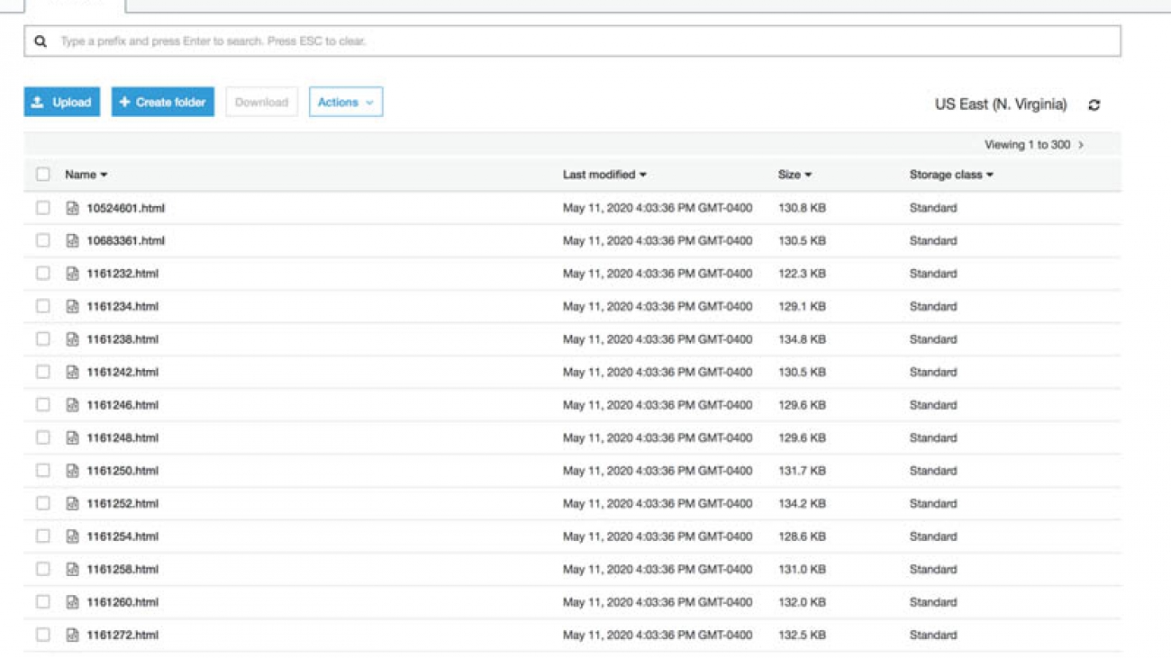
After the successful completion of the workflow, you can go to the Amazon S3 console and find an Amazon S3 bucket with the following directories:

/params.json    # Your parameters file.
/train/         # Where the training CSV files are stored
/history/       # Where the previous forecasts are stored
/history/raw/   # Contains the raw Amazon Forecast exported files
/history/clean/ # Contains the previous processed Amazon Forecast exported files
/quicksight/    # Contains the most updated forecasts according to the train dataset
/tmp/           # Where the Amazon Forecast files are temporarily stored before processing

The parameter file params.json stores attributes to call Forecast APIs from the Lambda functions. These parameter configurations contain information such as forecast type, predictor setting, and dataset setting, in addition to forecast domain, frequency, and dimension. For more information about API actions, see Amazon Forecast Service.

Now that your data is in Amazon S3, you can visualize your results.

Analyzing forecasted data with Athena and QuickSight

To complete your forecast pipeline, you need to query and visualize your data. Athena is an interactive query service that makes it easy to analyze data in Amazon S3 using standard SQL. QuickSight is a fast, cloud-powered business intelligence service that makes it easy to uncover insights through data visualization. To start analyzing your data, you first ingest your data into QuickSight using Athena as a data source.

If you’re new to AWS, set up QuickSight to create a QuickSight account. If you have an AWS account, subscribe to QuickSight to create an account.

If this is your first time using Athena on QuickSight, you have to give permissions to QuickSight to query Amazon S3 using Athena. For more information, see Insufficient Permissions When Using Athena with Amazon QuickSight.

  1. On the QuickSight console, choose New Analysis.
  2. Choose New Data Set.
  3. Choose Athena.
  4. In the New Athena data source window, for Data source name, enter a name; for example, Utility Prediction.
  5. Choose Validate connection.
  6. Choose Create data source.

The Choose your table window appears.

  1. Choose Use custom SQL.
  2. In the Enter custom SQL query window, enter a name for your query; for example, Query to merge Forecast result with training data.
  3. Enter the following code into the query text box:
    SELECT LOWER(forecast.item_id) as item_id,
             forecast.target_value,
             date_parse(forecast.timestamp, '%Y-%m-%d %H:%i:%s') as timestamp,
             forecast.type
    FROM default.forecast
    UNION ALL
    SELECT LOWER(train.item_id) as item_id,
             train.target_value,
             date_parse(train.timestamp, '%Y-%m-%d %H:%i:%s') as timestamp,
             'history' as type
    FROM default.train
    

  4. Choose Confirm query.

You now have the option to import your data to SPICE or query your data directly.

  1. Choose either option, then choose Visualize.

You see the following fields under Fields list:

  • item_id
  • target_value
  • timestamp
  • type

The exported forecast contains the following fields:

  • item_id
  • date
  • The requested quantiles (P10, P50, P90)

The type field contains the quantile type (P10, P50, P90) for your forecasted window and history as its value for your training data. This was done through the custom query to have a consistent historical line between your historical data and the exported forecast.

You can customize the quantiles by using the CreateForecast API optional parameter called ForecastType. For this post, you can configure this in the params.json file in Amazon S3.

  1. For X axis, choose timestamp.
  2. For Value, choose target_value.
  3. For Color, choose type.

In your parameters, you specified a 72-hour horizon. To visualize results, you need to aggregate the timestamp field on an hourly frequency.

  1. From the timestamp drop-down menu, choose Aggregate and Hour.

The following screenshot is your final forecast prediction. The graph shows a future projection in the quantiles p10, p50m, and p90, at which probabilistic forecasts are generated.

Conclusion

Every organization can benefit from more accurate forecasting to better predict product demand, optimize planning and supply chains, and more. Forecasting demand is a challenging task, and ML can narrow the gap between predictions and reality.

This post showed you how to create a repeatable, AI-powered, automated forecast generation process. You also learned how to implement an ML operation pipeline using serverless technologies and used a managed analytics service to get data insights by querying the data and creating a visualization.

There’s even more that you can do with Forecast. For more information about energy consumption predictions, see Making accurate energy consumption predictions with Amazon Forecast. For more information about quantiles, see Amazon Forecast now supports the generation of forecasts at a quantile of your choice.

If this post helps you or inspires you to solve a problem, share your thoughts and questions in the comments. You can use and extend the code on the GitHub repo.


About the Author

Luis Lopez Soria is an AI/ML specialist solutions architect working with the AWS machine learning team. He works with AWS customers to help them adopt machine learning on a large scale. He enjoys playing sports, traveling around the world, and exploring new foods and cultures.


Saurabh Shrivastava is a solutions architect leader and AI/ML specialist working with global systems integrators. He works with AWS partners and customers to provide them with architectural guidance for building scalable architecture in hybrid and AWS environments. He enjoys spending time with his family outdoors and traveling to new destinations to discover new cultures.


Pedro Sola Pimentel is an R&D solutions architect working with the AWS Brazil commercial team. He works with AWS to innovate and develop solutions using new technologies and services. He’s interested in recent computer science research topics and enjoys traveling and watching movies.


Read More

Enhancing enterprise search with Amazon Kendra

Enhancing enterprise search with Amazon Kendra

Amazon Kendra is an easy-to-use enterprise search service that allows you to add search capabilities to your applications so end-users can easily find information stored in different data sources within your company. This could include invoices, business documents, technical manuals, sales reports, corporate glossaries, internal websites, and more. You can harvest this information from storage solutions like Amazon Simple Storage Service (Amazon S3) and OneDrive; applications such as SalesForce, SharePoint and Service Now; or relational databases like Amazon Relational Database Service (Amazon RDS)

When you type a question, the service uses machine learning (ML) algorithms to understand the context and return the most relevant results, whether that’s a precise answer or an entire document. Most importantly, you don’t need to have any ML experience to do this—Amazon Kendra also provides you with the code that you need to easily integrate with your new or existing applications.

This post shows you how to create your internal enterprise search by using the capabilities of Amazon Kendra. This enables you to build a solution to create and query your own search index. For this post, you use Amazon.com help documents in HTML format as the data source, but Amazon Kendra also supports MS Office (.doc, .ppt), PDF, and text formats.

Overview of solution

This post provides the steps to help you create an enterprise search engine on AWS using Amazon Kendra. You can provision a new Amazon Kendra index in under an hour without much technical depth or ML experience.

The post also demonstrates how to configure Amazon Kendra for a customized experience by adding FAQs, deploying Amazon Kendra in custom applications, and synchronizing data sources. This post addresses and answers these questions in the subsequent sections.

Prerequisites

For this walkthrough, you should have the following prerequisites:

Creating and configuring your document repository

Before you can create an index in Amazon Kendra, you need to load documents into an S3 bucket. This section contains instructions to create an S3 bucket, get the files, and load them into the bucket. After completing all the steps in this section, you have a data source that Amazon Kendra can use.

  1. On the AWS Management Console, in the Region list, choose US East (N. Virginia) or any Region of your choice that Amazon Kendra is available in.
  2. Choose Services.
  3. Under Storage, choose S3.
  4. On the Amazon S3 console, choose Create bucket.
  5. Under General configuration, provide the following information:
    • Bucket name: kendrapost-{your account id}.
    • Region: Choose the same Region that you use to deploy your Amazon Kendra index (this post uses US East (N. Virginia) us-east-1).
  6. Under Bucket settings for Block Public Access, leave everything with the default values.
  7. Under Advanced settings, leave everything with the default values.
  8. Choose Create bucket.
  9. Download amazon_help_docs.zip and unzip the files.
  10. On the Amazon S3 console, select the bucket that you just created and choose Upload.
  11. Upload the unzipped files.

Inside your bucket, you should now see two folders: amazon_help_docs (with 3,100 objects) and faqs (with one object).

The following screenshot shows the contents of amazon_help_docs.

The following screenshot shows the contents of faqs.

Creating an index

An index is the Amazon Kendra component that provides search results for documents and frequently asked questions. After completing all the steps in this section, you have an index ready to consume documents from different data sources. For more information about indexes, see Index.

To create your first Amazon Kendra index, complete the following steps:

  1. On the console, choose Services.
  2. Under Machine Learning, choose Amazon Kendra.
  3. On the Amazon Kendra main page, choose Create an Index.
  4. In the Index details section, for Index name, enter kendra-blog-index.
  5. For Description, enter My first Kendra index.
  6. For IAM role, choose Create a new role.
  7. For Role name, enter -index-role (your role name has the prefix AmazonKendra-YourRegion-).
  8. For Encryption, don’t select Use an AWS KMW managed encryption key.

(Your data is encrypted with an Amazon Kendra-owned key by default.)

  1. Choose Next.

For more information about the IAM roles Amazon Kendra creates, see Prerequisites.

Amazon Kendra offers two editions. Kendra Enterprise Edition provides a high-availability service for production workloads. Kendra Developer Edition is suited for building a proof-of-concept and experimentation. For this post, you use the Developer edition.

  1. In the Provisioning editions section, select Developer edition.
  2. Choose Create.

For more information on the free tier, document size limits, and total storage for each Amazon Kendra edition, see Amazon Kendra pricing.

The index creation process can take up to 30 minutes. When the creation process is complete, you see a message at the top of the page that you successfully created your index.

Adding a data source

A data source is a location that stores the documents for indexing. You can synchronize data sources automatically with an Amazon Kendra index to make sure that searches correctly reflect new, updated, or deleted documents in the source repositories.

After completing all the steps in this section, you have a data source linked to Amazon Kendra. For more information, see Adding documents from a data source.

Before continuing, make sure that the index creation is complete and the index shows as Active.

  1. On the kendra-blog-index page, choose Add data sources.

Amazon Kendra supports six types of data sources: Amazon S3, SharePoint Online, ServiceNow, OneDrive, Salesforce online, and Amazon RDS. For this post, you use Amazon S3.

  1. Under Amazon S3, choose Add connector.

For more information about the different data sources that Amazon Kendra supports, see Adding documents from a data source.

  1. In the Define attributes section, for Data source name, enter amazon_help_docs.
  2. For Description, enter AWS services documentation.
  3. Choose Next.
  4. In the Configure settings section, for Enter the data source location, enter the S3 bucket you created: kendrapost-{your account id}.
  5. Leave Metadata files prefix folder location

By default, metadata files are stored in the same directory as the documents. If you want to place these files in a different folder, you can add a prefix. For more information, see S3 document metadata.

  1. For Select decryption key, leave it deselected.
  2. For Role name, enter source-role (your role name is prefixed with AmazonKendra-).
  3. For Additional configuration, you can add a pattern to include or exclude certain folders or files. For this post, keep the default values.
  4. For Frequency, choose Run on demand.

This step defines the frequency with which the data source is synchronized with the Amazon Kendra index. For this walkthrough, you do this manually (one time only).

  1. Choose Next.
  2. On the Review and create page, choose Create.
  3. After you create the data source, choose Sync now to synchronize the documents with the Amazon Kendra index.

The duration of this process depends on the number of documents that you index. For this use case, it may take 15 minutes, after which you should see a message that the sync was successful.

In the Sync run history section, you can see that 3,099 documents were synchronized.

Exploring the search index using the search console

The goal of this section is to let you explore possible search queries via the built-in Amazon Kendra console.

To search the index you created above, complete the following steps:

  1. Under Indexes, choose kendra-blog-index.
  2. Choose Search console.

Kendra can answer three types of questions: factoid, descriptive, and keyword. For more information, see Amazon Kendra FAQs. You can ask some questions using the Amazon.com help documents that you uploaded earlier.

In the search field, enter What is Amazon music unlimited?

With a factoid question (who, what, when, where), Amazon Kendra can answer and also offer a link to the source document.

As a keyword search, enter shipping rates to Canada. The following screenshot shows the answer Amazon Kendra gives.

Adding FAQs

You can also upload a list of FAQs to provide direct answers to common questions your end-users ask. To do this, you need to load a .csv file with the information related to the questions. This section contains instructions to create and configure that file and load it into Amazon Kendra.

  1. On the Amazon Kendra console, navigate to your index.
  2. Under Data management, choose FAQs.
  3. Choose Add FAQ.
  4. In the Define FAQ project section, for FAQ name, enter kendra-post-faq.
  5. For Description, enter My first FAQ list.

Amazon Kendra accepts .csv files formatted with each row beginning with a question followed by its answer. For example, see the following table.

Question Answer URL (optional)
What is the height of the Space Needle?  605 feet  https://www.spaceneedle.com/
How tall is the Space Needle?  605 feet  https://www.spaceneedle.com/
What is the height of the CN Tower? 1815 feet https://www.cntower.ca/
How tall is the CN Tower? 1815 feet https://www.cntower.ca/

This is how the .CSV file included for this use case looks like:

"How do I sign up for the Amazon Prime free Trial?"," To sign up for the Amazon Prime free trial, your account must have a current, valid credit card. Payment options such as an Amazon.com Corporate Line of Credit, checking accounts, pre-paid credit cards, or gift cards cannot be used. "," https://www.amazon.com/gp/help/customer/display.html/ref=hp_left_v4_sib?ie=UTF8&nodeId=201910190”
  1. Under FAQ settings, for S3, enter s3://kendrapost-{your account id}/faqs/kendrapost.csv.
  2. For IAM role, choose Create a new role.
  3. For Role name, enter faqs-role (your role name is prefixed with AmazonKendra-).
  4. Choose Add.
  5. Wait until you see the status show as Active.

You can now see how the FAQ works on the search console.

  1. Under Indexes, choose your index.
  2. Under Data management, choose Search console.
  3. In the search field, enter How do I sign up for the Amazon Prime free Trial?
  4. The following screenshot shows that Amazon Kendra added the FAQ that you uploaded previously to the results list, and provides an answer and a link to the related documentation.

Using Amazon Kendra in your own applications

You can add the following components from the search console in your application:

  • Main search page The main page that contains all the components. This is where you integrate your application with the Amazon Kendra API.
  • Search bar The component where you enter a search term and that calls the search function.
  • Results The component that displays the results from Amazon Kendra. It has three components: suggested answers, FAQ results, and recommended documents.
  • Pagination The component that paginates the response from Amazon Kendra.

Amazon Kendra provides source code that you can deploy in your website. This is offered free of charge under a modified MIT license so you can use it as is or change it for your own needs.

This section contains instructions to deploy Amazon Kendra search to your website. You use a Node.js demo application that runs locally in your machine. This use case is based on a MacOS environment.

To run this demo, you need the following components:

  1. Download amazon_aws-kendra-sample-app-master.zip and unzip the file.
  2. Open a terminal window and go to the aws-kendra-sample-app-master folder:
    cd /{folder path}/aws-kendra-sample-app-master

  3. Create a copy of the .env.development.local.example file as .env.development.local:
    cp .env.development.local.example .env.development.local

  4. Edit the .env.development.local file and add the following connection parameters:
    • REACT_APP_INDEX – Your Amazon Kendra index ID (you can find this number on the Index home page)
    • REACT_APP_AWS_ACCESS_KEY_ID – Your account access key
    • REACT_APP_AWS_SECRET_ACCESS_KEY – Your account secret access key
    • REACT_APP_AWS_SESSION_TOKEN – Leave it blank for this use case
    • REACT_APP_AWS_DEFAULT_REGION – The Region that you used to deploy the Kendra index (for example, us-east-1)
  5. Save the changes.
  6. Install the Node.js dependencies:
    npm install

  7. Launch the local development server:
    npm start

  8. View the demo app at http://localhost:3000/. You should see the following screenshot.
  9. Enter the same question you used to test the FAQs: How do I sign up for the Amazon Prime free Trial?

The following screenshot shows that the result is the same as the one you got from the Amazon Kendra console, even though the demo webpage is running locally in your machine.

Cleaning up

To avoid incurring future charges and to clean out unused roles and policies, delete the resources you created: the Amazon Kendra index, S3 bucket, and corresponding IAM roles.


  1. To delete the Amazon Kendra index, under Indexes, choose kendra-blog-index.
  2. In the index settings section, from the Actions drop-down menu, choose Delete.
  3. To confirm deletion, enter Delete in the field and choose Delete.

Wait until you get the confirmation message; the process can take up to 15 minutes.

For instructions on deleting your S3 bucket, see How do I delete an S3 Bucket?

Conclusion

In this post, you learned how to use Amazon Kendra to deploy an enterprise search service. You can use Amazon Kendra to improve the search experience in your company, powered by ML. You can enable rapid look for your documents using natural language, without any previous ML/AI experience. For more information about Amazon Kendra, see AWS re:Invent 2019 – Keynote with Andy Jassy on YouTube, Amazon Kendra FAQs, and What is Amazon Kendra?


About the Author

Leonardo Gómez is a Big Data Specialist Solutions Architect at AWS. Based in Toronto, Canada, He works with customers across Canada to design and build big data architectures.


Read More

Presenting a Challenge and Workshop in Efficient Open-Domain Question Answering

Presenting a Challenge and Workshop in Efficient Open-Domain Question Answering

Posted by Eunsol Choi, Visiting Faculty Researcher and Tom Kwiatkowski, Research Scientist, Google Research

One of the primary goals of natural language processing is to build systems that can answer a user’s questions. To do this, computers need to be able to understand questions, represent world knowledge, and reason their way to answers. Traditionally, answers have been retrieved from a collection of documents or a knowledge graph. For example, to answer the question, “When was the declaration of independence officially signed?” a system might first find the most relevant article from Wikipedia, and then locate a sentence containing the answer, “August 2, 1776”. However, more recent approaches, like T5, have also shown that neural models, trained on large amounts of web-text, can also answer questions directly, without retrieving documents or facts from a knowledge graph. This has led to significant debate about how knowledge should be stored for use by our question answering systems — in human readable text and structured formats, or in the learned parameters of a neural network.

Today, we are proud to announce the EfficientQA competition and workshop at NeurIPS 2020, organized in cooperation with Princeton University and the University of Washington. The goal is to develop an end-to-end question answering system that contains all of the knowledge required to answer open-domain questions. There are no constraints on how the knowledge is stored — it could be in documents, databases, the parameters of a neural network, or any other form — but entries will be evaluated based on the number of bytes used to access this knowledge, including code, corpora, and model parameters. There will also be an unconstrained track, in which the goal is to achieve the best possible question answering performance regardless of system size. To build small, yet robust systems, participants will have to explore new methods of knowledge representation and reasoning.

An illustration of how the memory budget changes as a neural network and retrieval corpus grow and shrink. It is possible that successful systems will also use other resources such as a knowledge graph.

Competition Overview
The competition will be evaluated using the open-domain variant of the Natural Questions dataset. We will also provide further human evaluation of all the top performing entries to account for the fact that there are many correct ways to answer a question, not all of which will be covered by any set of reference answers. For example, for the question “What type of car is a Jeep considered?” both “off-road vehicles” and “crossover SUVs” are valid answers.

The competition is divided between four separate tracks: best performing system under 500 Mb; best performing system under 6 Gb; smallest system to get at least 25% accuracy; and the best performing system with no constraints. The winners of each of these tracks will be invited to present their work during the competition track at NeurIPS 2020, which will be hosted virtually. We will also put each of the winning systems up against human trivia experts (the 2017 NeurIPS Human-Computer competition featured Jeopardy! and Who Wants to Be a Millionaire champions) in a real-time contest at the virtual conference.

Participation
To participate, go to the competition site where you will find the data and evaluation code available for download, as well as dates and instructions on how to participate, and a sign-up form for updates. Along with our academic collaborators, we have provided some example systems to help you get started.

We believe that the field of natural language processing will benefit from a greater exploration and comparison of small system question answering options. We hope that by encouraging the development of very small systems, this competition will pave the way for on-device question answering.

Acknowledgements
Creating this challenge and workshop has been a large team effort including Adam Roberts, Colin Raffel, Chris Alberti, Jordan Boyd-Graber, Jennimaria Palomaki, Kenton Lee, Kelvin Guu, and Michael Collins from Google; as well as Sewon Min and Hannaneh Hajishirzi from the University of Washington; and Danqi Chen from Princeton University.

RepNet: Counting Repetitions in Videos

RepNet: Counting Repetitions in Videos

Posted by Debidatta Dwibedi, Research Scientist, Robotics at Google

Repeating processes ranging from natural cycles, such as phases of the moon or heartbeats and breathing, to artificial repetitive processes, like those found on manufacturing lines or in traffic patterns, are commonplace in our daily lives. Beyond just their prevalence, repeating processes are of interest to researchers for the variety of insights one can tease out of them. It may be that there is an underlying cause behind something that happens multiple times, or there may be gradual changes in a scene that may be useful for understanding. Sometimes, repeating processes provide us with unambiguous “action units”, semantically meaningful segments that make up an action. For example, if a person is chopping an onion, the action unit is the manipulation action that is repeated to produce additional slices. These units may be indicative of more complex activity and may allow us to analyze more such actions automatically at a finer time-scale without having a person annotate these units. For the above reasons, perceptual systems that aim to observe and understand our world for an extended period of time will benefit from a system that understands general repetitions.

In “Counting Out Time: Class Agnostic Video Repetition Counting in the Wild”, we present RepNet, a single model that can understand a broad range of repeating processes, ranging from people exercising or using tools, to animals running and birds flapping their wings, pendulums swinging, and a wide variety of others. In contrast to our previous work, which used cycle-consistency constraints across different videos of the same action to understand them at a fine-grained level, in this work we present a system that can recognize repetitions within a single video. Along with this model, we are releasing a dataset to benchmark class-agnostic counting in videos and a Colab notebook to run RepNet.

RepNet
RepNet is a model that takes as input a video that contains periodic action of a variety of classes (including those unseen during training) and returns the period of repetitions found therein. In the past the problem of repetition counting has been addressed by directly comparing pixel intensities in frames, but real world videos have camera motion, occlusion by objects in the field, drastic scale difference and changes in form, which necessitates learning of features invariant to such noise. To accomplish this we train a machine learning model in an end-to-end manner to directly estimate the period of the repetitions. The model consists of three parts: a frame encoder, an intermediate representation, called a temporal self-similarity matrix (which we will describe below), and a period predictor.

First, the frame encoder uses the ResNet architecture as a per-frame model to generate embeddings of each frame of the video The ResNet architecture was chosen since it has been successful for a number of image and video tasks. Passing each frame of a video through a ResNet-based encoder yields a sequence of embeddings.

At this point we calculate a temporal self-similarity matrix (TSM) by comparing each frame’s embedding with every other frame in the video, returning a matrix that is easy for subsequent modules to analyze for counting repetitions. This process surfaces self-similarities in the stream of video frames that enable period estimation, as demonstrated in the video below.

Demonstration of how the TSM processes images of the Earth’s day-night cycle.

For each frame, we then use Transformers to predict the period of repetition and the periodicity (i.e., whether or not a frame is part of the periodic process) directly from the sequence of similarities in the TSM. Once we have the period, we obtain the per-frame count by dividing the number of frames captured in a periodic segment by the period length. We sum this up to predict the number of repetitions in the video.

Overview of the RepNet model.

Temporal Self-Similarity Matrix
The example of the TSM from the day-night cycle, shown above, is derived from an idealized scenario with fixed period repetitions. TSMs from real videos often reveal fascinating structures in the world, as demonstrated in the three examples below. Jumping jacks are close to the ideal periodic action with a fixed period, while in contrast, the period of a bouncing ball declines as the ball loses energy through repeated bounces. The video of someone mixing concrete demonstrates repetitive action that is preceded and followed by a period without motion. These three behaviors are clearly distinguished in the learned TSM, which requires that the model pay attention to fine changes in the scene.

Jumping Jacks (constant period; video from Kinetics), Bouncing ball (decreasing period; Kinetics), Mixing concrete (aperiodic segments present in video; PERTUBE dataset).

One advantage of using the TSM as an intermediate layer in RepNet is that the subsequent processing by the transformers is done in the self-similarity space and not in the feature space. This encourages generalization to unseen classes. For example, the TSMs produced by actions as different as jumping jacks or swimming are similar as long as the action was repeated at a similar pace. This allows us to train on some classes and yet expect generalization to unseen classes.

Data
One way to train the above model would be to collect a large dataset of videos that capture repetitive activities and label them with the repetition count. The challenge in this is two-fold. First, it requires one to examine a large number of videos to identify those with repeated actions. Following that, each video must be annotated with the number of times an action was repeated. While for certain tasks annotators can skip frames (for example, to classify a video as showing jumping jacks), they still need to see the entire video in order to count how many jumping jacks were performed.

We overcome this challenge by introducing a process for synthetic data generation that produces videos with repetitions using videos that may not contain repeating actions at all. This is accomplished by randomly selecting a segment of the video to repeat an arbitrary number of times, bookended by the original video context.

Our synthetic data generation pipeline that produces videos with repetitions from any video.

While this process generates a video that resembles a natural-looking video with repeating processes, it is still too simple for deep learning methods, which can learn to cheat by looking for artifacts, instead of learning to recognize repetitions. To address this, we perform extreme data augmentation, which we call camera motion augmentation. In this method, we modify the video to simulate a camera that smoothly moves around using 2D affine motion as the video progresses.

Left: An example of a synthetic repeating video generated from a random video. Right: An example of a video with camera motion augmentation, which is tougher for the model, but results in better generalization to real repeating videos (both from Kinetics).

Evaluation
Even though we can train a model on synthetic repeating videos, the resulting models must be able to generalize to real video of repeating processes. In order to evaluate the performance of the trained models on real videos, we collect a dataset of ~9000 videos from the Kinetics dataset. These videos span many action classes and capture diverse scenes, arising from the diversity of data seen on Youtube. We annotate these videos with the count of the action being repeated in the video. To encourage further research in this field, we are releasing the count annotations for this dataset, which we call Countix.

Applications
A class-agnostic counting model has many useful applications. RepNet serves as a single model that can count repetitions from many different domains:

RepNet can count repeated activities from a range of domains, such as slicing onions (left; video from Kinetics dataset), Earth’s diurnal cycle (middle; Himawari satellite data), or even a cheetah in motion (right; video from imgur.com).

RepNet could be used to estimate heartbeat rates from echocardiogram videos even though it has not seen such videos in training:

Predicted heart rates: 45 bpm (left) and 75 bpm (right). True heart rates 46-50 bpm and 78-79 bpm, respectively. RepNet’s prediction of the heart rate across different devices is encouragingly close to the rate measured by the device. (Source for left and right)

RepNet can also be used to monitor repeating activities for any changes in speed. Below we show how the Such changes in speed can also be used in other settings for quality or process control.

In this video, we see RepNet counting accelerating cellular oscillations observed under a laser microscope even though it has never seen such a video during training, (from Nature article).
Left: Person performing a “mountain climber” exercise. Right: The 1D projection of the RepNet embeddings using principal component analysis, capturing the moment that the person changes their speed during the exercise. (Video from Kinetics)

Release
We are releasing Countix annotations for the community to work on the problem of repetition counting. We are also releasing a Colab notebook for running RepNet. Using this you can run RepNet on your videos or even using your webcam to detect periodic activities in video and count repetitions automatically in videos.

Acknowledgements
This is joint work with Yusuf Aytar, Jonathan Tompson, Pierre Sermanet, and Andrew Zisserman. Special thanks to Tom Small for designing the visual explanation of TSM. The authors thank Anelia Angelova, Relja Arandjelović, Sourish Chaudhuri, Aishwarya Gomatam, Meghana Thotakuri, and Vincent Vanhoucke for their help with this project.

Scheduling Jupyter notebooks on SageMaker ephemeral instances

Scheduling Jupyter notebooks on SageMaker ephemeral instances

It’s 5 PM on a Friday. You’ve spent all afternoon coding out a complex, sophisticated feature engineering strategy. It just started working on your Amazon SageMaker Studio t3.medium notebook, and all you want to do is plug this onto a massive instance, scale it out over the rest of your dataset, and go home. You could upgrade your notebook instance, but the job would stop as soon as you close your laptop. Why not schedule the job from your notebook directly?

Amazon SageMaker provides a fully-managed solution for building, training, and deploying machine learning (ML) models. In this post, we demonstrate using Amazon SageMaker Processing Jobs to execute Jupyter notebooks with the open-source project Papermill. The combination of Amazon SageMaker with Amazon CloudWatch, AWS Lambda, and the entire AWS stack have always provided the modular backbone you need to scale up jobs, like feature engineering, both on the fly and on a schedule. We’re happy to provide a do-it-yourself toolkit to simplify this process, using AWS CloudFormation to set up permissions, Lambda to launch the job, and Amazon Elastic Container Registry (Amazon ECR) to create a customized execution environment. It includes a library and CLI to initiate notebook execution from any AWS client and a Jupyter plugin for a seamless user experience.

As of this writing, you can write code in a Jupyter notebook and run it on an Amazon SageMaker ephemeral instance with the click of a button, either immediately or on a schedule. With the tools provided here, you can do this from anywhere: at a shell prompt, in JupyterLab on Amazon SageMaker, in another JupyterLab environment you have, or automated in a program you’ve written. We’ve written sample code that simplifies setup by using AWS CloudFormation to handle the heavy lifting and provides convenience tools to run and monitor executions.

For more information about executing notebooks, see the GitHub repo. All the source code is available in aws-samples on GitHub. Read on to learn all about how to use scheduled notebook execution.

When to use this solution

This toolkit is especially useful for running nightly reports. For example, you may want to analyze all the training jobs your data science team ran that day, run a cost/benefit analysis, and generate a report about the business value your models are going to bring after you deploy them into production. That would be a perfect fit for a scheduled notebook—all the graphs, tables, and charts are generated by your code, the same as if you stepped through the notebook yourself, except now they are handled automatically, in addition to persisting in Amazon Simple Storage Service (Amazon S3). You can start your day with the latest notebook, executed overnight, to move your analysis forward.

Or, imagine that you want to scale up a feature engineering step. You’ve already perfected the for-loop to knock out all your Pandas transformations, and all you need is time and compute to run this on the full 20 GB of data. No problem—just drop your notebook into the toolkit, run a job, close your laptop, and you’re done. Your code continues to run on the scheduled instance, regardless of whether or not you’re actively using Jupyter at the moment.

Perhaps you’re on a data science team that still trains models on local laptops or Amazon SageMaker notebooks, and haven’t yet adopted the Amazon SageMaker ephemeral instances for training jobs. With this toolkit, you can easily use the advanced compute options only for the time you’re training a model. You can spin up a p3.xlarge only for the hour your model trains but use your Studio environment all day on the affordable t3.medium. You can easily connect these resources to the Experiments SDK with a few lines of code. Although it’s still fully supported to run Amazon SageMaker notebooks and Amazon SageMaker Studio on p3 instances, developing a habit of using the largest instances only for short periods is a net cost-savings exercise.

You may have an S3 bucket full of objects and need to run a full notebook on each object. These could be dates of phone call records in your call center or Tweet-streams from particular users in your social network. You can easily write a for-loop over those objects by using this toolkit, which schedules a job for each file, runs it on its dedicated instance, and stores the completed notebook in Amazon S3. These could even be model artifacts loaded in from your preferred training environment—package up your inference code in a notebook and use the toolkit to easily deploy them!

Finally, customers tell us that reporting on the performance of their models is a key asset for their stakeholders. With this toolkit, you can implement a human-in-the-loop solution that analyzes feature importance, produces ROC curves, and estimates how your model will perform on the tricky edge cases that are crucial to your final product. You can build a model profiler that all the data scientists on your team can easily access. You can trigger this model profiler to run after every training job is complete, closing the loop on the value of your analysis to your stakeholders.

Three Ways to Execute Notebooks on a Schedule in SageMaker

To execute a notebook in Amazon SageMaker, you use a Lambda function that sets up and runs an Amazon SageMaker Processing job. The function can be invoked directly by the user or added as a target of an Amazon EventBridge rule to run on a schedule or in response to an event. The notebook to run is stored as an Amazon S3 object so it’s available to run even if you’re not online when the execution happens. The following diagram illustrates this architecture.

We outline three different ways to install and use this capability that let you work with notebooks and schedules just the way you want.

Using the AWS APIs or CLI directly

You can use the AWS APIs directly to execute and schedule notebooks. To make the process easier, we have provided a CloudFormation template to set up the Lambda function you need and some AWS Identity and Access Management (IAM) roles and policies that you use when running notebooks. We also provided scripts for building and customizing the Docker container images that Amazon SageMaker Processing Jobs uses when running the notebooks.

After you instantiate the CloudFormation template and create a container image, you can run a notebook like this with the following code:

$ aws lambda invoke --function-name RunNotebook 
             --payload '{"input_path": "s3://mybucket/mynotebook.ipynb", 
                         "parameters": {"p": 0.75}}' result.json

To create a schedule, enter the following code, replacing the Region and account number in the arn, as well as the input_path to your S3 bucket.

$ aws events put-rule --name "RunNotebook-test" --schedule "cron(15 1 * * ? *)"
$ aws lambda add-permission --statement-id EB-RunNotebook-test 
                            --action lambda:InvokeFunction 
                            --function-name RunNotebook 
                            --principal events.amazonaws.com 
                            --source-arn arn:aws:events:us-east-1:123456789:rule/RunNotebook-test
$ aws events put-targets --rule RunNotebook-test 
                         --targets '[{"Id": "Default", 
                                      "Arn": "arn:aws:lambda:us-east-1:123456789:function:RunNotebook", 
                                      "Input": "{ "input_path": "s3://mybucket/mynotebook.ipynb", 
                                                  "parameters": {"p": 0.75}}"}]‘

With this approach, you manage moving the notebook to Amazon S3, monitoring Amazon SageMaker Processing Jobs, and retrieving the output notebook from Amazon S3.

This is a great solution when you’re a knowledgeable AWS user who wants to craft a solution without taking on extra dependencies. You can even modify the Lambda function we’ve written or the Papermill execution container to meet your exact needs.

For more information about scheduling notebooks with the AWS APIs, see the full setup instructions on the GitHub repo.

Making things easier with a convenience package

To make it easier to schedule notebooks (especially if you aren’t an AWS expert), we’ve created a convenience package that wraps the AWS tools in a CLI and Python library that give you a more natural interface to running and scheduling notebooks. This package lets you build customized execution environments without Docker, via AWS CodeBuild instead, and manages the Amazon S3 interactions and job monitoring for you.

After you run the setup, execute the notebook with the following code:

$ run-notebook run mynotebook.ipynb -p p=0.5 -p n=200

Schedule a notebook with the following code:

$ run-notebook schedule --at "cron(15 1 * * ? *)" --name nightly weather.ipynb -p "name=Boston, MA"

The convenience package also contains tools to monitor jobs and view schedules. See the following code:

$ run-notebook list-runs
Date                 Rule                 Notebook              Parameters           Status     Job
2020-06-15 15:31:40                       fraud-analysis.ipynb  name=Tom             Completed  papermill-fraud-analysis-2020-06-15-22-31-39
2020-06-15 01:00:08  DailyForecastSeattle DailyForecast.ipynb   place=Seattle, WA    Completed  papermill-DailyForecast-2020-06-15-08-00-08
2020-06-15 01:00:03  DailyForecastNewYork DailyForecast.ipynb   place=New York, NY   Completed  papermill-DailyForecast-2020-06-15-08-00-02
2020-06-12 22:34:06                       powers.ipynb          p=0.5                Completed  papermill-powers-2020-06-13-05-34-05
                                                                n=20
$ 

For more information about the convenience package, see the GitHub repo.

Executing notebooks directly from JupyterLab with a GUI

For those who prefer an interactive experience, the convenience package includes a JupyterLab extension that you can enable for JupyterLab running locally, in Amazon SageMaker Studio, or on an Amazon SageMaker notebook instance.

After you set up the Jupyter extension for Amazon SageMaker Studio users, you see the new notebook execution sidebar (the rocket ship icon). The sidebar lets you execute or schedule the notebook you’re viewing . You can use the notebook-runner container that was created by the default setup or any other container you built. Enter the ARN for the execution role these jobs utilize and your instance preference, and you’re ready to go!

After you choose Run Now, the Lambda function picks up your notebook and runs it on an Amazon SageMaker Processing job. You can view the status of that job by choosing Runs. See the following screenshot.

When the job is complete, the finished notebook is stored in Amazon S3. Remember, this means your previous runs will persist, so you can easily revert back to them.

Finally, import the output notebook by choosing View Output and Import Notebook. If you don’t import the notebook, it’s never copied to your local directory. This is great when you want to see what happened, but don’t want to clutter things up with lots of extra notebooks.

For instructions on setting up the JupyterLab extension and using the GUI to run and monitor your notebooks, see the GitHub repo.

Summary

This post discussed how you can combine the modular capabilities of Amazon SageMaker and the AWS cloud to give data scientists and ML engineers the seamless experience of running notebooks on ephemeral instances. We are releasing an open-source toolkit to simplify this process, including a CLI, convenience package, and Jupyter widget. We discussed a variety of use cases for this, from running nightly reports to scaling up feature engineering to profiling models on the latest datasets. We shared examples from the various ways of running the toolkit. Feel free to walk through the Quick Start on GitHub and step through even more examples on the GitHub repo.


Author Bios

Emily Webber is a machine learning specialist SA at AWS, who alternates between data scientist, machine learning architect, and research scientist based on the day of the week. She lives in Chicago, and you can find her on YouTube, LinkedIn, GitHub, or Twitch. When not helping customers and attempting to invent the next generation of machine learning experiences, she enjoys running along beautiful Lake Shore Drive, escaping into her Kindle, and exploring the road less traveled.


Tom Faulhaber is a Principal Engineer on the Amazon SageMaker team. Lately, he has been focusing on unlocking all the potential uses of the richness of Jupyter notebooks and how they can add to the data scientist’s toolbox in non-traditional ways. In his spare time, Tom is usually found biking and hiking to discover all the wild spaces around Seattle with his kids.


Read More

AWS DeepComposer Chartbusters: generate compositions in the style of Bach and compete to top the charts

AWS DeepComposer Chartbusters: generate compositions in the style of Bach and compete to top the charts

We are excited to announce the launch of AWS DeepComposer Chartbusters, a monthly challenge where developers can use AWS DeepComposer to create original compositions and compete to top the charts and win prizes. AWS DeepComposer gives developers a creative way to get started with machine learning (ML) and generative AI techniques. With AWS DeepComposer, developers, regardless of their background in ML, can get started with generative AI techniques to learn how to train and optimize their models to create original music. The first AWS DeepComposer Chartbusters challenge, Bach to the Future, requires developers to use a new generative AI algorithm provided in the AWS DeepComposer console to create compositions in the style of Bach.

Every month through October, 2020, AWS will release a new Chartbusters challenge that has a different monthly theme to introduce you to a variety of generative AI techniques. You don’t need any musical knowledge to participate in the challenge. Before participating in a challenge, you can use learning capsules available in the AWS DeepComposer console to learn the generative AI concepts required for each month’s challenge. Learning capsules provide easy-to-consume, bite-size content to help you learn the concepts of generative AI algorithms.

How to participate in the challenge

The challenge is open worldwide for developers to participate. To get started, you will need to use one of the generative AI algorithms available in the AWS DeepComposer console to create compositions. Once you are ready to submit your composition for the challenge, select Submit a composition in the console to submit your creations to SoundCloud. AWS DeepComposer will add your submission to the Chartbuster challenge playlist on SoundCloud.

You can invite your family and friends to listen and like your composition by using the social sharing buttons available on SoundCloud. At the end of each challenge period, AWS will shortlist the top 20 compositions using a sum of customer likes and count of plays on SoundCloud. Our human AWS experts and DeepComposer AI judge will evaluate the shortlist based on musical quality and creativity to select the top 10 ranked compositions. The DeepComposer AI judge is trained on original Bach compositions and scores how similar your composition is to Bach’s style.

At the end of each challenge period, we will announce the top 10 compositions in an AWS ML blog post and feature them in an exclusive AWS top 10 playlist on SoundCloud and in the AWS DeepComposer console. The winner for each month’s challenge will receive an AWS DeepComposer Chartbusters gold record mailed to their physical address. Additionally, we will interview the winner to share their experience and feature them in an AWS ML blog post. You can continue to participate in multiple challenges so that if you don’t make it to the top 10 in one challenge, you can participate in the next challenge for another chance to top the charts.

Bach to the Future challenge

The first AWS DeepComposer Chartbuster challenge titled Bach to the Future launches today and is open until July 25th. To participate in the challenge, you will need to use the autoregressive CNN (AR-CNN) algorithm available in the AWS DeepComposer console to create compositions in the style of Bach. AWS will announce the top 10 compositions for the Bach to the Future challenge and the theme for the next challenge on July 31st, 2020, in an AWS ML blog post.

The AR-CNN algorithm enhances the original input melody by adding or removing musical notes from the input melody. If the algorithm detects off-key or extraneous notes, it may choose to remove them. If it identifies additional specific notes that are highly probable in a Bach composition, it may decide to add them. Listen to the following example of a composition that is generated by applying the AR-CNN algorithm. You might recognize this tune from Jonathan Coulton, as it is available as a sample input melody in the AWS DeepComposer console.

Input: me-and-my-jar-with-extra-missing-notes.midi

Enhanced composition: me-and-my-jar-enhanced.midi

You can use the Introduction to autoregressive convolutional neural network learning capsule available in the AWS DeepComposer console to learn the concepts. To access the learning capsule in the console, navigate to learning capsules using the left navigation menu. Choose Introduction to autoregressive convolutional neural network to begin learning.

Creating and submitting a composition

To get started, log in to the AWS DeepComposer console and navigate to the music studio using the left navigation menu. You can use either the sample melodies provided in the console, record a custom melody using the keyboard, or import your own input track. You can adjust the tempo and pitch for your melody in the music studio.

Choose Autoregressive generative AI technique, and then choose Autoregressive CNN Bach model. You have four parameters that you can choose to adjust: Maximum notes to add, Maximum notes to remove, Sampling iterations, and Creative risk. For this example, let’s choose the defaults and select Enhance input melody.

The AR-CNN algorithm allows you to collaborate iteratively with the machine learning algorithm by experimenting with the parameters; you can use the output from one iteration of the AR-CNN algorithm as input to the next iteration.

To submit your composition for the challenge, choose Chartbusters using the left navigation menu, and select Submit a composition. Choose your composition from the drop-down menu, provide a track name for your composition, and select Submit. AWS DeepComposer will submit your composition to the Bach to the Future playlist on SoundCloud. You can select the Vote on SoundCloud button in the console to review and listen to other submissions for the challenge.

Congratulations! You have submitted your first entry for the AWS DeepComposer Chartbusters challenge. Invite your friends and family to listen to and like your composition.

To celebrate the launch of the first Chartbuster challenge, we are offering the AWS DeepComposer keyboard at a special price of $79 for a limited period from 6/23/2020 to 7/15/2020 on amazon.com. The pricing includes the keyboard and a 3-month free trial of AWS DeepComposer services.

Learn more about AWS DeepComposer Chartbusters at https://aws.amazon.com/deepcomposer/chartbusters.


About the Author

Jyothi Nookula is a Principal Product Manager for AWS AI devices. She loves to build products that delight her customers. In her spare time, she loves to paint and host charity fund raisers for her art exhibitions.


Read More

Spotlight session with PhD students from the 2019 Facebook Fellowship cohort

Spotlight session with PhD students from the 2019 Facebook Fellowship cohort

Each year, we invite PhD students from around the world to apply for the Facebook Fellowship, a program designed to encourage and support promising doctoral students who are engaged in innovative and relevant research in areas related to computer science and engineering.

As a continuation of our regular Fellowship spotlight series, we’re highlighting Aishwarya Ganesan (University of Wisconsin–Madison), Kartik Hegde (University of Illinois at Urbana-Champaign), Maria Bauza Villalonga (Massachusetts Institute of Technology), and Neil Gaikwad (Massachusetts Institute of Technology). From teaching robots to identify objects to developing human-centered AI and public policy for sustainable development, these four Fellows showcase a wide array of research areas.

Improving the reliability of distributed systems without compromising performance

Aishwarya Ganesan is a PhD candidate in computer sciences at the University of Wisconsin–Madison (UW–Madison), advised by Professor Andrea Arpaci-Dusseau and Professor Remzi Arpaci-Dusseau. Her research interests are in distributed systems, storage and file systems, and operating systems, with a focus on improving the reliability of distributed systems without compromising their performance.

“I’ve always been fascinated by distributed systems,” she says. “And the reliability and performance challenges are especially interesting at the scale of Facebook with multiple applications and millions of users.” In February, Aishwarya and her team at UW–Madison won a Facebook research award in distributed systems with their proposal entitled “BlockCheck: Examining and improving blockchain reliability.”

Aishwarya learned about the Facebook Fellowship program at OSDI. “One of the main reasons I applied [to the program] was the opportunity to be part of a cohort of peers who are likely to be my future colleagues in academia or industry,” she says. She also appreciates having connections to Fellows from previous years who could provide PhD guidance and practical advice such as what the interview process after graduation is like.

“Winning the Facebook Fellowship also gives me an opportunity to interact with Facebook researchers and engineers. Through these interactions, I hope to learn how the ideas developed as part of my thesis are applicable in the real world.”

Aishwarya’s research has been recognized with a Best Paper award at FAST 2020 and FAST 2018 and a Best Paper award nomination at FAST 2017. She was selected for the Rising Stars in EECS 2018 workshop. Read more on her webpage.

Accelerating deep learning on mobile and IoT devices

Kartik Hegde is a PhD student at the University of Illinois at Urbana-Champaign, advised by Chris Fletcher. He received a bachelor of technology degree from National Institute of Technology Karnataka (NITK), Surathkal, in 2015. His research is focused on building efficient chips to power next-generation AI workloads.

Every day, we interact with smart devices that offer information and convenience through services hosted in the cloud — but this requires a constant internet connection, and response times can be slow. Kartik’s research aims to build more efficient processors that enable more machine learning on the device, faster and more cost effectively.

Before Kartik became a Fellow, he spent some time as an intern at Facebook and experienced what it’s like to conduct research in industry. “At Facebook, we get the best of what academia and industry offer,” he explains. “In academia, you have the independence to pursue your own ideas. In industry, you get the satisfaction of having an impact on people. If your idea is built into something at Facebook, it’s impacting billions of people. It’s the best of both worlds.”

The Fellowship Award includes a paid visit to Facebook HQ in Menlo Park for the annual Fellowship Summit, where Fellows may present their current research in a poster session to discuss their ideas with other Fellows as well as Facebook researchers. “It’s a great privilege where you meet all of the other Fellows and get a chance to network and hear great talks,” says Kartik, who attended the 2019 Fellowship Summit. “I was inspired by conversations I had with other Fellows about new ideas and possibilities for collaboration.”

Although the event won’t be held in person this year, the Fellows will still get a chance to connect with each other remotely. “In addition to the benefit of making new connections, the Fellowship also offers the recognition of winning a competitive fellowship and the independence to work on your own projects,” Kartik says.

To learn more about Kartik and his research, visit his webpage.

Teaching robots to identify objects by combining tactile sensors with computer vision

Maria Bauza Villalonga is a PhD student in robotics at Massachusetts Institute of Technology, working with Professor Alberto Rodriguez. She received bachelor’s degrees in mathematics and in physics from Polytechnic University of Catalonia in Spain. Her research focuses on combining tactile and visual information to enhance robot dexterity during object manipulation.

“In industry automation, many processes involve picking up objects and performing tasks,” Maria explains. “While it’s trivial for a human to identify an object through touch, it requires a lot of intelligence for a robot to pick up an object from a bin and accurately localize it in order to perform the next task. There are many cases where industry cannot yet use robots because of this challenge.”

Maria’s goal is to improve a robot’s ability to accurately manipulate objects and perform tasks by combining computer vision with tactile sensing information. With her MIT-Princeton team, Maria won the Amazon Robotics Challenge stowing task in 2017 and received the Amazon Robotics Best Systems Paper Award in Manipulation in 2018. She explains that through this competition, they learned about the importance of tactile localization for a robot to be able to estimate where an object is.

In her research, the robot uses tactile sensors to scan and reason about the object it is touching and combines that with computer vision to accurately identify and localize objects. She is using tools that Facebook has developed for image recognition and segmentation in her research.

When she finishes her PhD, Maria plans to apply for a faculty position. She enjoys academia because she can think long-term and work on projects that could take years to accomplish, and explore her original ideas with her students. Learn more about Maria’s research on her website.

Advancing sustainable development with just design of human-centered AI and public policy

Neil Gaikwad is a doctoral student in the MIT Media Lab at the Massachusetts Institute of Technology, working with Professor Danielle Wood. He specializes in human-centered machine learning and public policy for sustainable development. Neil develops data-driven human-AI collaboration algorithms and social computing systems, with a focus on increasing fairness and transparency in high-stakes policy decisions.

“Over the centuries, socio-technical systems such as market institutions and humanitarian systems have been instrumental in socioeconomic and environmental sustainability. However, lack of scientific understanding of underlying social and physical processes often leads to prejudiced policy decisions that harm vulnerable communities and hinder sustainable development,” Neil explains. “My research seeks to decode the fundamental nature of these processes on sustainability through the lens of human-centered machine learning, participatory design, and evidence-based policymaking.”

Neil became interested in the Fellowship because of the high-impact research of Facebook Core Data Science (CDS), which aligned with his research agenda. Neil and Facebook CDS have created the first workshop on Humanitarian Mapping at the ACM KDD conference. “The ongoing crisis of the COVID-19 pandemic exemplifies the criticality of the workshop. This initiative will create a framework for researchers to showcase how industry, academics, government research labs, and policymakers can work together to address humanitarian and sustainability challenges,” he says.

Neil is also a recipient of the Karl Taylor Compton Prize (MIT’s highest student award) and is an MIT Arts Scholar. He harnesses contemporary photography to communicate and advocate for science. “It’s hard to contextualize sustainability challenges such as climate change to a general audience merely through scientific models,” he says. “The arts play a vital role in helping people understand scientific underpinnings at subconscious levels and facilitate inclusive dialogues and engagement between diverse communities.”

After graduation, Neil plans to pursue a career in a line of academic research as a professor. “My major goal is to establish an informed research agenda at the boundaries of computational, design, and socioeconomic thinking, with students and global collaborators, to address the pressing sustainable development problems,” he says. For more information about Neil’s work, visit his webpage and arts portfolio.

The post Spotlight session with PhD students from the 2019 Facebook Fellowship cohort appeared first on Facebook Research.

Read More

Cynthia Breazeal named Media Lab associate director

Cynthia Breazeal has been promoted to full professor and named associate director of the Media Lab, joining the two other associate directors: Hiroshi Ishii and Andrew Lippman. Both appointments are effective July 1.

In her new associate director role, Breazeal will work with lab faculty and researchers to develop new strategic research initiatives. She will also play a key role in exploring new funding mechanisms to support broad Media Lab needs, including multi-faculty research efforts, collaborations with other labs and departments across the MIT campus, and experimental executive education opportunities. 

“I am excited that Cynthia will be applying her tremendous energy, creativity, and intellect to rally the community in defining new opportunities for funding and research directions,” says Pattie Maes, chair of the lab’s executive committee. “As a first step, she has already organized a series of informal charrettes, where all members of the lab community can participate in brainstorming collaborations that range from tele-creativity, to resilient communities, to sustainability and climate change.” 

Most recently, Breazeal has led an MIT collaboration between the Media Lab, MIT Stephen A. Schwarzman College of Computing, and MIT Open Learning to develop aieducation.mit.edu, an online learning site for grades K-12, which shares a variety of online activities for students to learn about artificial intelligence, with a focus on how to design and use AI responsibly. 

While assuming these new responsibilities, Breazeal will continue to head the lab’s Personal Robots research group, which focuses on developing personal social robots and their potential for meaningful impact on everyday life — from educational aids for children, to pediatric use in hospitals, to at-home assistants for the elderly.

Breazeal is globally recognized as a pioneer in human-robot interaction. Her book, “Designing Sociable Robots” (MIT Press, 2002), is considered pivotal in launching the field. In 2019 she was named an AAAI fellow. Previously, she received numerous awards including the National Academy of Engineering’s Gilbreth Lecture Award and MIT Technology Review‘s TR100/35 Award. Her robot Jibo was on the cover of TIME magazine in its Best Inventions list of 2017, and in 2003 she was a finalist for the National Design Awards in Communications Design. In 2014, Fortune magazine recognized her as one of the Most Promising Women Entrepreneurs. The following year, she was named one of Entrepreneur magazine’s Women to Watch.

Breazeal earned a BS in electrical and computer engineering from the University of California at Santa Barbara, and MS and ScD degrees from MIT in electrical engineering and computer science.

Read More