Monthly Archives: June 2020

Sometimes it’s hard to find the right words to describe what you’re looking for. As the adage goes, “A picture is worth a thousand words.” Often, it’s easier to show a physical example or image than to try to describe an item with words, especially when using a search engine to find what you’re looking for.

In this post, you build a visual image search application from scratch in under an hour, including a full-stack web application for serving the visual search results.

Visual search can improve customer engagement in retail businesses and e-commerce, particularly for fashion and home decoration retailers. Visual search allows retailers to suggest thematically or stylistically related items to shoppers, which retailers would struggle to achieve by using a text query alone. According to Gartner, “By 2021, early adopter brands that redesign their websites to support visual and voice search will increase digital commerce revenue by 30%.”

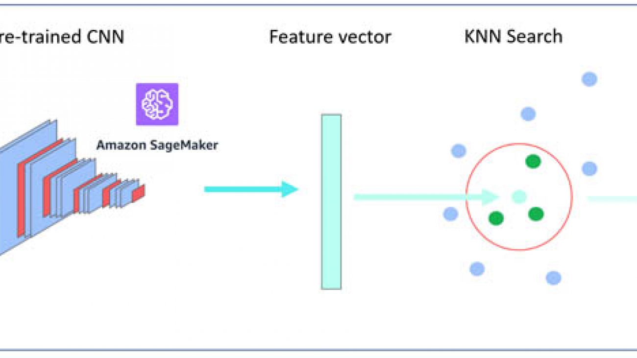
High-level example of visual searching

Amazon SageMaker is a fully managed service that provides every developer and data scientist with the ability to build, train, and deploy machine learning (ML) models quickly. Amazon Elasticsearch Service (Amazon ES) is a fully managed service that makes it easy for you to deploy, secure, and run Elasticsearch cost-effectively at scale. Amazon ES offers k-Nearest Neighbor (KNN) search, which can enhance search in similar use cases such as product recommendations, fraud detection, and image, video, and semantic document retrieval. Built using the lightweight and efficient Non-Metric Space Library (NMSLIB), KNN enables high-scale, low-latency, nearest neighbor search on billions of documents across thousands of dimensions with the same ease as running any regular Elasticsearch query.

The following diagram illustrates the visual search architecture.

Overview of solution

Implementing the visual search architecture consists of two phases:

1. Building a reference KNN index on Amazon ES from a sample image dataset.
2. Submitting a new image to the Amazon SageMaker endpoint and Amazon ES to return similar images.

KNN reference index creation

In this step, from each image you extract 2,048 feature vectors from a pre-trained Resnet50 model hosted in Amazon SageMaker. Each vector is stored to a KNN index in an Amazon ES domain. For this use case, you use images from FEIDEGGER, a Zalando research dataset consisting of 8,732 high-resolution fashion images. The following screenshot illustrates the workflow for creating KNN index.

The process includes the following steps:

1. Users interact with a Jupyter notebook on an Amazon SageMaker notebook instance.
2. A pre-trained Resnet50 deep neural net from Keras is downloaded, the last classifier layer is removed, and the new model artifact is serialized and stored in Amazon Simple Storage Service (Amazon S3). The model is used to start a TensorFlow Serving API on an Amazon SageMaker real-time endpoint.
3. The fashion images are pushed through the endpoint, which runs the images through the neural network to extract the image features, or embeddings.
4. The notebook code writes the image embeddings to the KNN index in an Amazon ES domain.

Visual search from a query image

In this step, you present a query image from the application, which passes through the Amazon SageMaker hosted model to extract 2,048 features. You use these features to query the KNN index in Amazon ES. KNN for Amazon ES lets you search for points in a vector space and find the “nearest neighbors” for those points by Euclidean distance or cosine similarity (the default is Euclidean distance). When it finds the nearest neighbors vectors (for example, k = 3 nearest neighbors) for a given image, it returns the associated Amazon S3 images to the application. The following diagram illustrates the visual search full-stack application architecture.

The process includes the following steps:

1. The end-user accesses the web application from their browser or mobile device.
2. A user-uploaded image is sent to Amazon API Gateway and AWS Lambda as a base64 encoded string and is re-encoded as bytes in the Lambda function.
   1. A publicly readable image URL is passed as a string and downloaded as bytes in the function.
3. The bytes are sent as the payload for inference to an Amazon SageMaker real-time endpoint, and the model returns a vector of the image embeddings.
4. The function passes the image embedding vector in the search query to the k-nearest neighbor in the index in the Amazon ES domain. A list of k similar images and their respective Amazon S3 URIs is returned.
5. The function generates pre-signed Amazon S3 URLs to return back to the client web application, used to display similar images in the browser.

AWS services

To build the end-to-end application, you use the following AWS services:

• AWS Amplify – AWS Amplify is a JavaScript library for front-end and mobile developers building cloud-enabled applications. For more information, see the GitHub repo.
• Amazon API Gateway – A fully managed service to create, publish, maintain, monitor, and secure APIs at any scale.
• AWS CloudFormation – AWS CloudFormation gives developers and businesses an easy way to create a collection of related AWS and third-party resources and provision them in an orderly and predictable fashion.
• Amazon ES – A managed service that makes it easy to deploy, operate, and scale Elasticsearch clusters at scale.
• AWS IAM – AWS Identity and Access Management (IAM) enables you to manage access to AWS services and resources securely.
• AWS Lambda – An event-driven, serverless computing platform that runs code in response to events and automatically manages the computing resources the code requires.
• Amazon SageMaker – A fully managed end-to-end ML platform to build, train, tune, and deploy ML models at scale.
• AWS SAM– AWS Serverless Application Model (AWS SAM) is an open-source framework for building serverless applications.
• Amazon S3 – An object storage service that offers an extremely durable, highly available, and infinitely scalable data storage infrastructure at very low cost.

Prerequisites

For this walkthrough, you should have an AWS account with appropriate IAM permissions to launch the CloudFormation template.

Deploying your solution

You use a CloudFormation stack to deploy the solution. The stack creates all the necessary resources, including the following:

• An Amazon SageMaker notebook instance to run Python code in a Jupyter notebook
• An IAM role associated with the notebook instance
• An Amazon ES domain to store and retrieve image embedding vectors into a KNN index
• Two S3 buckets: one for storing the source fashion images and another for hosting a static website

From the Jupyter notebook, you also deploy the following:

• An Amazon SageMaker endpoint for getting image feature vectors and embeddings in real time.
• An AWS SAM template for a serverless back end using API Gateway and Lambda.
• A static front-end website hosted on an S3 bucket to demonstrate a real-world, end-to-end ML application. The front-end code uses ReactJS and the Amplify JavaScript library.

To get started, complete the following steps:

1. Sign in to the AWS Management Console with your IAM user name and password.
2. Choose Launch Stack and open it in a new tab:
   
3. On the Quick create stack page, select the check box to acknowledge the creation of IAM resources.
4. Choose Create stack.
   
5. Wait for the stack to complete executing.

You can examine various events from the stack creation process on the Events tab. When the stack creation is complete, you see the status CREATE_COMPLETE.

You can look on the Resources tab to see all the resources the CloudFormation template created.

6. On the Outputs tab, choose the SageMakerNotebookURL value.

This hyperlink opens the Jupyter notebook on your Amazon SageMaker notebook instance that you use to complete the rest of the lab.

You should be on the Jupyter notebook landing page.

7. Choose visual-image-search.ipynb.
   

Building a KNN index on Amazon ES

For this step, you should be at the beginning of the notebook with the title Visual image search. Follow the steps in the notebook and run each cell in order.

You use a pre-trained Resnet50 model hosted on an Amazon SageMaker endpoint to generate the image feature vectors (embeddings). The embeddings are saved to the Amazon ES domain created in the CloudFormation stack. For more information, see the markdown cells in the notebook.

Continue when you reach the cell Deploying a full-stack visual search application in your notebook.

The notebook contains several important cells.

To load a pre-trained ResNet50 model without the final CNN classifier layer, see the following code (this model is used just as an image feature extractor):

#Import Resnet50 model
model = tf.keras.applications.ResNet50(weights='imagenet', include_top=False,input_shape=(3, 224, 224),pooling='avg')

You save the model as a TensorFlow SavedModel format, which contains a complete TensorFlow program, including weights and computation. See the following code:

#Save the model in SavedModel format
model.save('./export/Servo/1/', save_format='tf')

Upload the model artifact (model.tar.gz) to Amazon S3 with the following code:

#Upload the model to S3
sagemaker_session = sagemaker.Session()
inputs = sagemaker_session.upload_data(path='model.tar.gz', key_prefix='model')
inputs

You deploy the model into an Amazon SageMaker TensorFlow Serving-based server using the Amazon SageMaker Python SDK. The server provides a super-set of the TensorFlow Serving REST API. See the following code:

#Deploy the model in Sagemaker Endpoint. This process will take ~10 min.
from sagemaker.tensorflow.serving import Model

sagemaker_model = Model(entry_point='inference.py', model_data = 's3://' + sagemaker_session.default_bucket() + '/model/model.tar.gz',
                        role = role, framework_version='2.1.0', source_dir='./src' )

predictor = sagemaker_model.deploy(initial_instance_count=3, instance_type='ml.m5.xlarge')

Extract the reference images features from the Amazon SageMaker endpoint with the following code:

# define a function to extract image features
from time import sleep

sm_client = boto3.client('sagemaker-runtime')
ENDPOINT_NAME = predictor.endpoint

def get_predictions(payload):
    return sm_client.invoke_endpoint(EndpointName=ENDPOINT_NAME,
                                           ContentType='application/x-image',
                                           Body=payload)

def extract_features(s3_uri):
    key = s3_uri.replace(f's3://{bucket}/', '')
    payload = s3.get_object(Bucket=bucket,Key=key)['Body'].read()
    try:
        response = get_predictions(payload)
    except:
        sleep(0.1)
        response = get_predictions(payload)

    del payload
    response_body = json.loads((response['Body'].read()))
    feature_lst = response_body['predictions'][0]
    
    return s3_uri, feature_lst

You define Amazon ES KNN index mapping with the following code:

#Define KNN Elasticsearch index mapping
knn_index = {
    "settings": {
        "index.knn": True
    },
    "mappings": {
        "properties": {
            "zalando_img_vector": {
                "type": "knn_vector",
                "dimension": 2048
            }
        }
    }
}

Import the image feature vector and associated Amazon S3 image URI into the Amazon ES KNN Index with the following code:

# defining a function to import the feature vectors corrosponds to each S3 URI into Elasticsearch KNN index
# This process will take around ~3 min.


def es_import(i):
    es.index(index='idx_zalando',
             body={"zalando_img_vector": i[1], 
                   "image": i[0]}
            )
    
process_map(es_import, result, max_workers=workers)

Building a full-stack visual search application

Now that you have a working Amazon SageMaker endpoint for extracting image features and a KNN index on Amazon ES, you’re ready to build a real-world full-stack ML-powered web app. You use an AWS SAM template to deploy a serverless REST API with API Gateway and Lambda. The REST API accepts new images, generates the embeddings, and returns similar images to the client. Then you upload a front-end website that interacts with your new REST API to Amazon S3. The front-end code uses Amplify to integrate with your REST API.

1. In the following cell, prepopulate a CloudFormation template that creates necessary resources such as Lambda and API Gateway for full-stack application:

   s3_resource.Object(bucket, 'backend/template.yaml').upload_file('./backend/template.yaml', ExtraArgs={'ACL':'public-read'})
   
   
   sam_template_url = f'https://{bucket}.s3.amazonaws.com/backend/template.yaml'
   
   # Generate the CloudFormation Quick Create Link
   
   print("Click the URL below to create the backend API for visual search:n")
   print((
       'https://console.aws.amazon.com/cloudformation/home?region=us-east-1#/stacks/create/review'
       f'?templateURL={sam_template_url}'
       '&stackName=vis-search-api'
       f'&param_BucketName={outputs["s3BucketTraining"]}'
       f'&param_DomainName={outputs["esDomainName"]}'
       f'&param_ElasticSearchURL={outputs["esHostName"]}'
       f'&param_SagemakerEndpoint={predictor.endpoint}'
   ))
   

   The following screenshot shows the output: a pre-generated CloudFormation template link.

2. Choose the link.

You are sent to the Quick create stack page.

3. Select the check boxes to acknowledge the creation of IAM resources, IAM resources with custom names, and CAPABILITY_AUTO_EXPAND.
4. Choose Create stack.

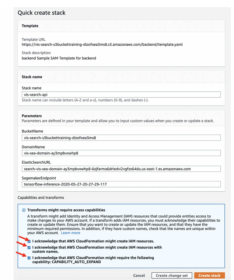
After the stack creation is complete, you see the status CREATE_COMPLETE. You can look on the Resources tab to see all the resources the CloudFormation template created.

5. After the stack is created, proceed through the cells.

The following cell indicates that your full-stack application, including front-end and back-end code, are successfully deployed:

print('Click the URL below:n')
print(outputs['S3BucketSecureURL'] + '/index.html')

The following screenshot shows the URL output.

6. Choose the link.

You are sent to the application page, where you can upload an image of a dress or provide the URL link of a dress and get similar dresses.

7. When you’re done testing and experimenting with your visual search application, run the last two cells at the bottom of the notebook:

   # Delete the endpoint
   predictor.delete_endpoint()
   
   # Empty S3 Contents
   training_bucket_resource = s3_resource.Bucket(bucket)
   training_bucket_resource.objects.all().delete()
   
   hosting_bucket_resource = s3_resource.Bucket(outputs['s3BucketHostingBucketName'])
   hosting_bucket_resource.objects.all().delete()
   

   These cells terminate your Amazon SageMaker endpoint and empty your S3 buckets to prepare you for cleaning up your resources.

Cleaning up

To delete the rest of your AWS resources, go to the AWS CloudFormation console and delete the vis-search-api and vis-search stacks.

Conclusion

In this post, we showed you how to create an ML-based visual search application using Amazon SageMaker and the Amazon ES KNN index. You used a pre-trained Resnet50 model trained on an ImageNet dataset. However, you can also use other pre-trained models, such as VGG, Inception, and MobileNet, and fine-tune with your own dataset.

A GPU instance is recommended for most deep learning purposes. Training new models is faster on a GPU instance than a CPU instance. You can scale sub-linearly when you have multi-GPU instances or if you use distributed training across many instances with GPUs. However, we used CPU instances for this use case so that you can complete the walkthrough under the AWS Free Tier.

For more information about the code sample in the post, see the GitHub repo. For more information about Amazon ES, see the following:

• How can I improve indexing performance on my Elasticsearch cluster?
• Amazon Elasticseach Service Best Practices
• Reducing cost for small Amazon Elasticsearch Service domains

About the Authors

Amit Mukherjee is a Sr. Partner Solutions Architect with AWS. He provides architectural guidance to help partners achieve success in the cloud. He has a special interest in AI and machine learning. In his spare time, he enjoys spending quality time with his family.

Laith Al-Saadoon is a Sr. Solutions Architect with a focus on data analytics at AWS. He spends his days obsessing over designing customer architectures to process enormous amounts of data at scale. In his free time, he follows the latest in machine learning and artificial intelligence.

Read More

XGBoost is a popular and efficient machine learning (ML) algorithm for regression and classification tasks on tabular datasets. It implements a technique known as gradient boosting on trees and performs remarkably well in ML competitions.

Since its launch, Amazon SageMaker has supported XGBoost as a built-in managed algorithm. For more information, see Simplify machine learning with XGBoost and Amazon SageMaker. As of this writing, you can take advantage of the open-source Amazon SageMaker XGBoost container, which has improved flexibility, scalability, extensibility, and Managed Spot Training. For more information, see the Amazon SageMaker sample notebooks and sagemaker-xgboost-container on GitHub, or see XBoost Algorithm.

This post introduces the benefits of the open-source XGBoost algorithm container and presents three use cases.

Benefits of the open-source SageMaker XGBoost container

The new XGBoost container has following benefits:

Latest version

The open-source XGBoost container supports the latest XGBoost 1.0 release and all improvements, including better performance scaling on multi-core instances and improved stability for distributed training.

Flexibility

With the new script mode, you can now customize or use your own training script. This functionality, which is also available for TensorFlow, MXNet, PyTorch, and Chainer users, allows you to add in custom pre- or post-processing logic, run additional steps after the training process, or take advantage of the full range of XGBoost functions (such as cross-validation support). You can still use the no-script algorithm mode (like other Amazon SageMaker built-in algorithms), which only requires you to specify a data location and hyperparameters.

Scalability

The open-source container has a more efficient implementation of distributed training, which allows it to scale out to more instances and reduces out-of-memory errors.

Extensibility

Because the container is open source, you can extend, fork, or modify the algorithm to suit your needs, beyond using the script mode. This includes installing additional libraries and changing the underlying version of XGBoost.

Managed Spot Training

You can save up to 90% on your Amazon SageMaker XGBoost training jobs with Managed Spot Training support. This fully managed option lets you take advantage of unused compute capacity in the AWS Cloud. Amazon SageMaker manages the Spot Instances on your behalf so you don’t have to worry about polling for capacity. The new version of XGBoost automatically manages checkpoints for you to make sure your job finishes reliably. For more information, see Managed Spot Training in Amazon SageMaker and Use Checkpoints in Amazon SageMaker.

Additional input formats

XGBoost now includes support for Parquet and Recordio-protobuf input formats. Parquet is a standardized, open-source, self-describing columnar storage format for use in data analysis systems. Recordio-protobuf is a common binary data format used across Amazon SageMaker for various algorithms, which XGBoost now supports for training and inference. For more information, see Common Data Formats for Training. Additionally, this container supports Pipe mode training for these data formats. For more information, see Using Pipe input mode for Amazon SageMaker algorithms.

Using the latest XGBoost container as a built-in algorithm

As an existing Amazon SageMaker XGBoost user, you can take advantage of the new features and improved performance by specifying the version when you create your training jobs. For more information about getting started with XGBoost or using the latest version, see the GitHub repo.

You can upgrade to the new container by specifying the framework version (1.0-1). This version specifies the upstream XGBoost framework version (1.0) and an additional Amazon SageMaker version (1). If you have an existing XGBoost workflow based on the legacy 0.72 container, this is the only change necessary to get the same workflow working with this container. The container also supports XGBoost 0.90 by using version as 0.90-1.

See the following code:

from sagemaker.amazon.amazon_estimator import get_image_uri
container = get_image_uri(region, 'xgboost', '1.0-1')

estimator = sagemaker.estimator.Estimator(container, 
                                          role, 
                                          hyperparameters=hyperparameters,
                                          train_instance_count=1, 
                                          train_instance_type='ml.m5.2xlarge', 
                                          )

estimator.fit(training_data)

Using managed Spot Instances

You can also take advantage of managed Spot Instance support by enabling the train_use_spot_instances flag on your Estimator. For more information, see the GitHub repo.

When you are training with managed Spot Instances, the training job may be interrupted, which causes it to take longer to start or finish. If a training job is interrupted, you can use a checkpointed snapshot to resume from a previously saved point, which can save training time (and cost). You can also use the checkpoint_s3_uri, which is where your training job stores snapshots, to seamlessly resume when a Spot Instance is interrupted. See the following code:

estimator = sagemaker.estimator.Estimator(container, 
                                          role, 
                                          hyperparameters=hyperparameters,
                                          train_instance_count=1, 
                                          train_instance_type='ml.m5.2xlarge', 
                                          output_path=output_path, 
                                          sagemaker_session=sagemaker.Session(),
                                          train_use_spot_instances=train_use_spot_instances, 
                                          train_max_run=train_max_run, 
                                          train_max_wait=train_max_wait,
                                          checkpoint_s3_uri=checkpoint_s3_uri
                                         )
                                         
estimator.fit({'train': train_input})                                         

Towards the end of the job, you should see the following two lines of output:

• Training seconds: X – The actual compute time your training job
• Billable seconds: Y – The time you are billed for after you apply Spot discounting

If you enabled train_use_spot_instances, you should see a notable difference between X and Y, which signifies the cost savings from using Managed Spot Training. This is reflected in the following code:

Managed Spot Training savings: (1-Y/X)*100 %

Using script mode

Script mode is a new feature with the open-source Amazon SageMaker XGBoost container. You can use your own training or hosting script to fully customize the XGBoost training or inference workflow. The following code example is a walkthrough of using a customized training script in script mode. For more information, see the GitHub repo.

Preparing the entry-point script

A typical training script loads data from the input channels, configures training with hyperparameters, trains a model, and saves a model to model_dir so it can be hosted later. Hyperparameters are passed to your script as arguments and can be retrieved with an argparse.ArgumentParser instance.

Starting with the main guard, use a parser to read the hyperparameters passed to your Amazon SageMaker estimator when creating the training job. These hyperparameters are made available as arguments to your input script. You also parse several Amazon SageMaker-specific environment variables to get information about the training environment, such as the location of input data and where to save the model. See the following code:

if __name__ == '__main__':
    parser = argparse.ArgumentParser()

    # Hyperparameters are described here
    parser.add_argument('--num_round', type=int)
    parser.add_argument('--max_depth', type=int, default=5)
    parser.add_argument('--eta', type=float, default=0.2)
    parser.add_argument('--objective', type=str, default='reg:squarederror')
    
    # Sagemaker specific arguments. Defaults are set in the environment variables.
    parser.add_argument('--train', type=str, default=os.environ['SM_CHANNEL_TRAIN'])
    parser.add_argument('--validation', type=str, default=os.environ['SM_CHANNEL_VALIDATION'])
    
    args = parser.parse_args()
    
    train_hp = {
        'max_depth': args.max_depth,
        'eta': args.eta,
        'gamma': args.gamma,
        'min_child_weight': args.min_child_weight,
        'subsample': args.subsample,
        'silent': args.silent,
        'objective': args.objective
    }
    
    dtrain = xgb.DMatrix(args.train)
    dval = xgb.DMatrix(args.validation)
    watchlist = [(dtrain, 'train'), (dval, 'validation')] if dval is not None else [(dtrain, 'train')]

    callbacks = []
    prev_checkpoint, n_iterations_prev_run = add_checkpointing(callbacks)
    # If checkpoint is found then we reduce num_boost_round by previously run number of iterations
    
    bst = xgb.train(
        params=train_hp,
        dtrain=dtrain,
        evals=watchlist,
        num_boost_round=(args.num_round - n_iterations_prev_run),
        xgb_model=prev_checkpoint,
        callbacks=callbacks
    )
    
    model_location = args.model_dir + '/xgboost-model'
    pkl.dump(bst, open(model_location, 'wb'))
    logging.info("Stored trained model at {}".format(model_location))

Inside the entry-point script, you can optionally customize the inference experience when you use Amazon SageMaker hosting or batch transform. You can customize the following:

• input_fn() – How the input is handled
• predict_fn() – How the XGBoost model is invoked
• output_fn() – How the response is returned

The defaults work for this use case, so you don’t need to define them.

Training with the Amazon SageMaker XGBoost estimator

After you prepare your training data and script, the XGBoost estimator class in the Amazon SageMaker Python SDK allows you to run that script as a training job on the Amazon SageMaker managed training infrastructure. You also pass the estimator your IAM role, the type of instance you want to use, and a dictionary of the hyperparameters that you want to pass to your script. See the following code:

from sagemaker.session import s3_input
from sagemaker.xgboost.estimator import XGBoost

xgb_script_mode_estimator = XGBoost(
    entry_point="abalone.py",
    hyperparameters=hyperparameters,
    image_name=container,
    role=role, 
    train_instance_count=1,
    train_instance_type="ml.m5.2xlarge",
    framework_version="1.0-1",
    output_path="s3://{}/{}/{}/output".format(bucket, prefix, "xgboost-script-mode"),
    train_use_spot_instances=train_use_spot_instances,
    train_max_run=train_max_run,
    train_max_wait=train_max_wait,
    checkpoint_s3_uri=checkpoint_s3_uri
)

xgb_script_mode_estimator.fit({"train": train_input})

Deploying the custom XGBoost model

After you train the model, you can use the estimator to create an Amazon SageMaker endpoint—a hosted and managed prediction service that you can use to perform inference. See the following code:

predictor = xgb_script_mode_estimator.deploy(initial_instance_count=1, instance_type="ml.m5.xlarge")
test_data = xgboost.DMatrix('/path/to/data')
predictor.predict(test_data)

Training with Parquet input

You can now train the latest XGBoost algorithm with Parquet-formatted files or streams directly by using the Amazon SageMaker supported open-sourced ML-IO library. ML-IO is a high-performance data access library for ML frameworks with support for multiple data formats, and is installed by default on the latest XGBoost container. For more information about importing a Parquet file and training with it, see the GitHub repo.

Conclusion

The open-source XGBoost container for Amazon SageMaker provides a fully managed experience and additional benefits that save you money in training and allow for more flexibility.

About the Authors

Rahul Iyer is a Software Development Manager at AWS AI. He leads the Framework Algorithms team, building and optimizing machine learning frameworks like XGBoost and Scikit-learn. Outside work, he enjoys nature photography and cherishes time with his family.

Rocky Zhang is a Senior Product Manager at AWS SageMaker. He builds products that help customers solve real world business problems with Machine Learning. Outside of work he spends most of his time watching, playing, and coaching soccer.

Eric Kim is an engineer in the Algorithms & Platforms Group of Amazon AI. He helps support the AWS service SageMaker, and has experience in machine learning research, development, and application. Outside of work, he is a music lover and a fan of all dogs.

Laurence Rouesnel is a Senior Manager in Amazon AI. He leads teams of engineers and scientists working on deep learning and machine learning research and products, like SageMaker AutoPilot and Algorithms. In his spare time he’s an avid fan of traveling, table-top RPGs, and running.

Read More

It’s quite common to be watching a soccer match and, when seeing a player score a goal, surmise how difficult scoring that goal was. Your opinions may be further confirmed if you’re watching the match on television and hear the broadcaster exclaim how hard it was for that shot to find the back of the net. Previously, it was based on the naked eye and colored with assumptions based on the number of defenders present, where the goalkeeper was, or if a player was in front of the net or angled to the side. Now, with xGoals (short for “Expected Goals”), one of the Bundesliga Match Facts powered by AWS, it’s possible to put data and insights behind the wow factor, showing the fans the exact probability of a player scoring a goal when shooting from any position on the playing field.

Deutsche Fußball Liga (DFL) is responsible for the organization and marketing of Germany’s professional soccer league, Bundesliga and Bundesliga 2. In every match, DFL collects more than 3.6 million data points for deeper insights into what’s happening on the playing field. The vision is to become the most innovative sports league by enhancing the experiences of over 500 million Bundesliga fans and more than 70 media partners around the globe. DFL aims to achieve its vision by using technology in new ways to provide real-time statistics driven by machine learning (ML), build personalized content for the fans, and turn data into insights and action.

xGoals is one of the two new Match Facts (Average Positions being the second) that DFL and AWS officially launched at the end of May 2020, enhancing global fan engagement with Germany’s Bundesliga, the top soccer league in the country, and the league with the highest average number of goals per match. Using Amazon SageMaker, a fully managed service to build, train, and deploy ML models, xGoals can objectively evaluate the goal-scoring chances of Bundesliga players shooting from any position on the playing field. xGoals can also determine if a pass helped open up a better opportunity than if the player had taken a shot or passed the ball to a player in a better position to shoot.

xGoals and other Bundesliga Match Facts are setting new standards by providing data-driven insights in the world of soccer.

Quantifying goal-scoring chances

The xGoals Match Facts debuted on May 26, 2020, during the Borussia Dortmund vs. FC Bayern Munich match, which was broadcast in over 200 countries worldwide. In a game where little was given away and everything had to be fought for, FC Bayern Munich’s Joshua Kimmich managed to take a remarkable shot. Given the distance to goal, angle of the strike, number of surrounding players, and other factors, his goal-scoring probability in this specific situation was only 6%.

The xGoals ML model produces a probability figure between 0 and 1, after which the values are displayed as a percentage. For example, an evaluation of ML models trained on Bundesliga matches showed that every penalty kick has an xGoals (or “xG”) value of 0.77—meaning that the goal-scoring probability is 77%. xGoals introduces a value that qualitatively measures the utilization of goal-scoring chances of a player or a team and provides information about their performance.

At the end of each match, an aggregation of xGoals values by both teams is also shown. This way, viewers get an objective metric of goal-scoring chances. The particular match mentioned before had a high probability of a draw, if not for that one successful shot from Kimmich. xGoals can enhance the viewing experience and provide insights in several ways, keeping fans engaged and enabling them to understand the potential of players and teams throughout a match or a season.

Given the highly dynamic circumstances around scoring attempts prior to a goal, it’s very hard to achieve an xG value above 70%. Player positions constantly change, and players must make split-second decisions with limited information, mostly relying on intuition. Thus, even when positioned in close proximity to the goal, depending on the situation, the difficulty to score may vary significantly. Therefore, it’s important to have a data-driven, holistic view of all the events on the playing field at any given moment. Only then is it possible to make accurate predictions by also taking into account other players’ positions when feeding this information into the xGoals ML model.

It all starts with data

To bring Match Facts to life, several checks and processes happen before, during, and after a match. Various stakeholders are involved in data acquisition, data processing, graphics, content creation (such as TV feed editing), and live commentary. Each one of the Bundesliga soccer stadiums is equipped with up to 20 cameras for automatic optical tracking of player and ball positions. An editorial team processes additional video data and picks the ideal camera angles and scenes to broadcast. This also includes the decision of when exactly to display Match Facts on TV.

Nearly all match events, such as penalty kicks and shots at goals, are documented live and sent to the DFL systems for remote verification. Human annotators categorize and supplement events with additional situation-specific information. For example, they can add player and team assignments and the type of the shot taken (such as blocking or assisting).

Eventually, all the raw match data is ingested into the Bundesliga Match Facts system on AWS to calculate the xGoals values, which are then distributed worldwide for broadcasting.

In the case of the official Bundesliga app and website, Match Facts are continuously displayed on end-user devices as soon as possible. The same applies to other external customers of DFL with third-party digital platforms, which also offer the latest insights and advanced statistics to soccer fans around the globe.

Real-time content distribution and fan engagement are especially important now, because Bundesliga matches are being played in empty stadiums, which has impacted the in-person soccer viewing experience.

Our ML journey: Bringing code to production

DFL’s leadership, management, and developers have been working hand-in-hand with AWS Professional Services Teams through this cloud-adoption journey, enabling ML for an enhanced viewer experience. The mission of AWS Data Science consultants is to accelerate customer business outcomes through the effective use of ML. Customer engagements start with an initial assessment and taking a closer look at desired outcomes and feasibility from both a business and technical perspective. AWS Professional Services consultants supplement customers’ existing teams with specialized skill sets and industry experience, developing proof of concepts (POCs), minimal viable products (MVPs), and bringing ML solutions to production. At the same time, continued learning and knowledge transfer drive sustainable and directly attributable business value.

In addition to in-house experimentations and prototyping performed at DFL’s subsidiary Sportec Solutions, a well-established research community is already working on refining the performance and accuracy of xGoals calculations. Combining this domain knowledge with the right tech stack and establishing best practices allows for faster innovation and execution at scale while ensuring operational excellence, security, reliability, performance efficiency, and cost optimization.

Historical soccer match data is the foundation of state-of-the-art ML-based xGoals model-training approaches. We can use this data to train ML models to infer xGoals outcomes based on given conditions on the playing field. For data quality evaluations and initial experimentations, we need to perform exploratory data analysis, data visualization, data transformation, and data validation. As an example, this can be done in Amazon SageMaker notebooks. The next natural step is to move the ML workloads from research to development. Deploying ML models to production requires an interdisciplinary engineering approach involving a combination of data engineering, data science, and software development. Production settings require error handling, failover, and recovery plans. Overall, ML system development and operations (MLOps) necessitates code refactoring, re-engineering and optimization, automation, setting up the foundational cloud infrastructure, implementing DevOps and security patterns, end-to-end testing, monitoring, and proper system design. The goal should always be to automate as many system components as possible to minimize manual intervention and reduce the need for maintenance.

In the next sections, we further explore the tech stack behind the Bundesliga Match Facts powered by AWS and underlying considerations when streamlining the path to bring xGoals to production.

xGoals model training with Amazon SageMaker

Traditional xGoals ML models are based on event data only. This means that only the approximate position of a player and their distance to a goal are taken into account when evaluating goal-scoring chances. In the case of the Bundesliga, shot-at-goal events are combined with additional high-precision positional data obtained with a 25 Hz frame rate. This comes with additional overhead in data cleaning and data preprocessing within the necessary data stream analytics pipeline. However, the benefits of having more accurate results clearly outweigh the necessary engineering effort and complexity introduced. Based on the ball and player positions, which are constantly being tracked, the model can determine an array of additional features, such as the distance of a player to the goal, angle to the goal, a player’s speed, number of defenders in the line of shot, and goalkeeper coverage.

For xGoals, we used the Amazon SageMaker XGBoost algorithm to train an ML model on over 40,000 historical shots at goals in the Bundesliga since 2017. This can either be performed with the default training script (XGBoost as a built-in algorithm) or extended by adding preprocessing and postprocessing scripts (XGBoost as a framework). The Amazon SageMaker Python SDK makes it easy to perform training programmatically with built-in scaling. It also abstracts away the complexity of resource deployment and management needed for automatic XGBoost hyperparameter optimization. It’s advisable to start developing with small subsets of the available data for faster experimentation and gradually evolve and optimize towards more complex ML models trained on the full dataset.

An xGoals training job consists of a binary classification task with Area Under the ROC Curve (AUC) as the objective metric and a highly imbalanced training and validation dataset of shots at goals, which either did or didn’t lead to a goal being scored.

Given the various ML model candidates from the Bayesian search-based hyperparameter optimization job, the best-performing one is picked for deployment on an Amazon SageMaker endpoint. Due to differing resource requirements and longevity, ML model training is decoupled from hosting. The endpoint can be invoked from within applications such as AWS Lambda functions or from within Amazon SageMaker notebooks using an API call for real-time inference.

However, training an ML model using Amazon SageMaker isn’t enough. Other infrastructure components are necessary to handle the full cloud ML pipeline, which consists of data integration, data cleaning, data preprocessing, feature engineering, and ML model training and deployment. In addition, other application-specific cloud components need to be integrated.

xGoals architecture: Serverless ML

Before designing application architecture, we put a continuous integration and continuous delivery/deployment (CI/CD) pipeline in place. In accordance with the guidelines stated in the AWS Well-Architected Framework whitepaper, we followed a multi-account setup approach for independent development, staging, and production CI/CD pipeline stages. We paired this with an infrastructure as code (IaC) approach to provision these environments and have predictable deployments for each code change. This allows the team to have segregate environments, reduces release cycles, and facilitates testability of code. After the developer tools were in place, we started to draft the architecture for the application. The following diagram illustrates this architecture.

Data is ingested in two separate ways: AWS Fargate is used for (serverless compute engines for containers) receiving positional and event data streams, and Amazon API Gateway for receiving additional metadata such as team compositions and player names. This incoming data triggers a Lambda function. This Lambda function takes care of a variety of short-lived, one-time tasks such as automatic de-provisioning of idle resources; data preprocessing; simple extract, transform, and load (ETL) jobs; and several data quality tests that occur every time new match data is consumed. We also use Lambda to invoke the Amazon SageMaker endpoint to retrieve the xGoals predictions given a set of input features.

We use two databases to store the match states: Amazon DynamoDB, a key-value database, and Amazon DocumentDB (with MongoDB compatibility), a document database. The latter makes it easy to query and index position and event data in JSON format with nested structures. This is especially suitable if workloads require a flexible schema for fast, iterative development. For central storage of official match data, we use Amazon Simple Storage Service (Amazon S3). Amazon S3 stores the historical data from all match days, which is used to iteratively improve the xGoals model. Amazon S3 also stores metadata on model performance, model monitoring, and security metrics.

To monitor the performance of the application, we use an AWS Amplify web application. This gives the operations team and business stakeholders an overview of the system health and status of Match Facts calculations and its underlying cloud infrastructure in the form of a user-friendly dashboard. Such operational insights are important to capture and incorporate in post-match retrospective analyses to ensure continuous improvements of the current system. This dashboard also allows us to collect metrics to measure and evaluate the achievement of desired business outcomes. Continuous monitoring of relevant KPIs, such as overall system load and performance, end-to-end latency, and other non-functional requirements, ensures a holistic view of the current system from both business and technical perspectives.

The xGoals architecture is built in a fully serverless fashion for improved scalability and ease of use. Fully-managed services remove the undifferentiated heavy lifting of managing servers and other basic infrastructure components. The architecture allows us to dynamically support demand when matches start and release the resources at the end of the game without the need for manual actions, which reduces application costs and operational overhead.

Summary

Since naming AWS as its official technology provider in January 2020, the Bundesliga and AWS have embarked on a journey together to bring advanced analytics to life for soccer fans and broadcasters in over 200 countries. Bundesliga Match Facts powered by AWS helps audiences better understand the strategy involved in decision-making on the pitch. xGoals allows soccer viewers to quantitatively evaluate goal-scoring probabilities based on several conditions on the playing field. Other use cases include scoring chances aggregations in the form of individual players’ and goalkeepers’ performance metrics, and objective evaluations of whether or not the scoreline in a match is a fair reflection of what took place on the playing field.

AWS Professional Services has been working hand-in-hand with DFL and its subsidiary Sportec Solutions, advancing its digital transformation, accelerating business outcomes, and ensuring continuous innovation. Over the course of the coming seasons, DFL will introduce new Bundesliga Match Facts powered by AWS to keep fans engaged, entertained, and provide them with a world-class soccer viewing experience.

“We at Bundesliga are able to use this advanced technology from AWS, including statistics, analytics, and machine learning, to interpret the data and deliver more in-depth insights and better understanding of the split-second decisions made on the pitch. The use of Bundesliga Match Facts enables viewers to gain deeper insights into the key decisions in each match.”

— Andreas Heyden, Executive Vice President of Digital Innovations for the DFL Group

About the Authors

Marcelo Aberle is a Data Scientist in the AWS Professional Services team, working with customers to accelerate their business outcomes through the use of AI/ML. He was the lead developer of the Bundesliga Match Facts xGoals. He enjoys traveling for extended periods of time and is an avid admirer of minimalist design and architecture.

Mirko Janetzke is the Head of IT Development at Sportec Solutions GmbH, the DFL subsidiary responsible for data gathering, data and statistics systems, and soccer analytics within the DFL group. Mirko loves soccer and has been following the Bundesliga and his home team since he was a young boy. In his spare time, he likes to go hiking in the Bavarian Alps with his family and friends.

Lina Mongrand is a Senior Enterprise Services Manager at AWS Professional Services. Lina focuses on helping Media & Entertainment customers build their cloud strategies and approaches and guiding them through their transformation journeys. She is passionate about emerging technologies such as AI/ML and especially how these can help customers achieve their business outcomes. In her spare time, Lina enjoys mountaineering in the nearby Alps (she lives in Munich) with friends and family.

Read More

Named entity recognition (NER) involves sifting through text data to locate noun phrases called named entities and categorizing each with a label, such as person, organization, or brand. For example, in the statement “I recently subscribed to Amazon Prime,” Amazon Prime is the named entity and can be categorized as a brand. Building an accurate in-house custom entity recognizer can be a complex process, and requires preparing large sets of manually annotated training documents and selecting the right algorithms and parameters for model training.

This post explores an end-to-end pipeline to build a custom NER model using Amazon SageMaker Ground Truth and Amazon Comprehend.

Amazon SageMaker Ground Truth enables you to efficiently and accurately label the datasets required to train machine learning systems. Ground Truth provides built-in labeling workflows that take human labelers step-by-step through tasks and provide tools to efficiently and accurately build the annotated NER datasets required to train machine learning (ML) systems.

Amazon Comprehend is a natural language processing (NLP) service that uses machine learning to find insights and relationships in text. Amazon Comprehend processes any text file in UTF-8 format. It develops insights by recognizing the entities, key phrases, language, sentiments, and other common elements in a document. To use this custom entity recognition service, you need to provide a dataset for model training purposes, with either a set of annotated documents or a list of entities and their type label (such as PERSON) and a set of documents containing those entities. The service automatically tests for the best and most accurate combination of algorithms and parameters to use for model training.

The following diagram illustrates the solution architecture.

The end-to-end process is as follows:

1. Upload a set of text files to Amazon Simple Storage Service (Amazon S3).
2. Create a private work team and a NER labeling job in Ground Truth.
3. The private work team labels all the text documents.
4. On completion, Ground Truth creates an augmented manifest named manifest in Amazon S3.
5. Parse the augmented output manifest file and create the annotations and documents file in CSV format, which is acceptable by Amazon Comprehend. We mainly focus on a pipeline that automatically converts the augmented output manifest file, and this pipeline can be one-click deployed using an AWS CloudFormation In addition, we also show how to use the convertGroundtruthToComprehendERFormat.sh script from the Amazon Comprehend GitHub repo to parse the augmented output manifest file and create the annotations and documents file in CSV format. Although you need only one method for the conversion, we highly encourage you to explore both options.
6. On the Amazon Comprehend console, launch a custom NER training job, using the dataset generated by the AWS Lambda

To minimize the time spent on manual annotations while following this post, we recommend using the small accompanying corpus example. Although this doesn’t necessarily lead to performant models, you can quickly experience the whole end-to-end process, after which you can further experiment with larger corpus or even replace the Lambda function with another AWS service.

Setting up

You need to install the AWS Command Line Interface (AWS CLI) on your computer. For instructions, see Installing the AWS CLI.

You create a CloudFormation stack that creates an S3 bucket and the conversion pipeline. Although the pipeline allows automatic conversions, you can also use the conversion script directly and the setup instructions described later in this post.

Setting up the conversion pipeline

This post provides a CloudFormation template that performs much of the initial setup work for you:

• Creates a new S3 bucket
• Creates a Lambda function with Python 3.8 runtime and a Lambda layer for additional dependencies
• Configures the S3 bucket to auto-trigger the Lambda function on arrivals of output.manifest files

The pipeline source codes are hosted in the GitHub repo. To deploy from the template, in another browser window or tab, sign in to your AWS account in us-east-1.

Launch the following stack:

Complete the following steps:

1. For Amazon S3 URL, enter the URL for the template.
2. Choose Next.
   
3. For Stack name, enter a name for your stack.
4. For S3 Bucket Name, enter a name for your new bucket.
5. Leave the remaining parameters at their default.
6. Choose Next.
   
7. On the Configure stack options page, choose Next.
   
8. Review your stack details.
   
9. Select the three check-boxes acknowledging that AWS CloudFormation might create additional resources and capabilities.
10. Choose Create stack.
    

CloudFormation is now creating your stack. When it completes, you should see something like the following screenshot.

Setting up the conversion script

To set up the conversion script on your computer, complete the following steps:

1. Download and install Git on your computer.
2. Decide where you want to store the repository on your local machine. We recommend making a dedicated folder so you can easily navigate to it using the command prompt later.
3. In your browser, navigate to the Amazon Comprehend GitHub repo.
4. Under Contributors, choose Clone or download.
5. Under Clone with HTTPS, choose the clipboard icon to copy the repo URL.

To clone the repository using an SSH key, including a certificate issued by your organization’s SSH certificate authority, choose Use SSH and choose the clipboard icon to copy the repo URL to your clipboard.

6. In the terminal, navigate to the location in which you want to store the cloned repository. You can do so by entering $ cd <directory>.
7. Enter the following code:

   $ git clone <repo-url>

After you clone the repository, follow the steps in the README file on how to use the script to integrate the Ground Truth NER labeling job with Amazon Comprehend custom entity recognition.

Uploading the sample unlabeled corpus

Run the following commands to copy the sample data files to your S3 bucket:

$ aws s3 cp s3://aws-ml-blog/artifacts/blog-groundtruth-comprehend-ner/sample-data/groundtruth/doc-00.txt s3://<your-bucket>/raw/

$ aws s3 cp s3://aws-ml-blog/artifacts/blog-groundtruth-comprehend-ner/sample-data/groundtruth/doc-01.txt s3://<your-bucket>/raw/

$ aws s3 cp s3://aws-ml-blog/artifacts/blog-groundtruth-comprehend-ner/sample-data/groundtruth/doc-02.txt s3://<your-bucket>/raw/

The sample data shortens the time you spent annotating, and isn’t necessarily optimized for best model performance.

Running the NER labeling job

This step involves three manual steps:

1. Create a private work team.
2. Create a labeling job.
3. Annotate your data.

You can reuse the private work team over different jobs.

When the job is complete, it writes an output.manifest file, which a Lambda function picks up automatically. The function converts this augmented manifest file into two files: .csv and .txt. Assuming that the output manifest is s3://<your-bucket>/gt/<gt-jobname>/manifests/output/output.manifest, the two files for Amazon Comprehend are located under s3://<your-bucket>/gt/<gt-jobname>/manifests/output/comprehend/.

Creating a private work team

For this use case, you form a private work team with your own email address as the only worker. Ground Truth also allows you to use Amazon Mechanical Turk or a vendors workforce.

1. On the Amazon SageMaker console, under Ground Truth, choose Labeling workforces.
2. On the Private tab, choose Create private team.
   
3. For Team name, enter a name for your team.
   
4. For Add workers, select Invite new workers by email.
5. For Email addresses, enter your email address.
6. For Organization name, enter a name for your organization.
7. For Contact email, enter your email.
8. Choose Create private team.
   
9. Go to the new private team to find the URL of the labeling portal.
   
   You also receive an enrollment email with the URL, user name, and a temporary password, if this is your first time being added to this team (or if you set up Amazon Simple Notification Service (Amazon SNS) notifications).
10. Sign in to the labeling URL.
    
11. Change the temporary password to a new password.
    

Creating a labeling job

The next step is to create a NER labeling job. This post highlights the key steps. For more information, see Adding a data labeling workflow for named entity recognition with Amazon SageMaker Ground Truth.

To reduce the amount of annotation time, use the sample corpus that you have copied to your S3 bucket as the input to the Ground Truth job.

1. On the Amazon SageMaker console, under Ground Truth, choose Labeling jobs.
2. Choose Create labeling job.
   
3. For Job name, enter a job name.
4. Select I want to specify a label attribute name different from the labeling job name.
5. For Label attribute name, enter ner.
6. Choose Create manifest file.
   

This step lets Ground Truth automatically convert your text corpus into a manifest file.

A pop-up window appears.

7. For Input dataset location, enter the Amazon S3 location.
8. For Data type, select Text.
9. Choose Create.
   

You see a message that your manifest is being created.

10. When the manifest creation is complete, choose Create.
    

You can also prepare the input manifest yourself. Be aware that the NER labeling job requires its input manifest in the {"source": "embedded text"} format rather than the refer style {"source-ref": "s3://bucket/prefix/file-01.txt"}. In addition, the generated input manifest automatically detects line break n and generates one JSON line per line per document, whereas if you generate it on your own, you may decide for one JSON line per document (although you may still need to preserve the n for your downstream).

11. For IAM role, choose the role the CloudFormation template created.
    
12. For Task selection, choose Named entity recognition.
13. Choose Next.
    
14. On the Select workers and configure tool page, for Worker types, select Private.
15. For Private teams, choose the private work team you created earlier.
    
16. For Number of workers per dataset object, make sure the number of workers (1) matches the size of your private work team.
17. In the text box, enter labeling instructions.
18. Under Labels, add your desired labels. See the next screenshot for the labels needed for the recommended corpus.
19. Choose Create.
    

The job has been created, and you can now track the status of the individual labeling tasks on the Labeling jobs page.

The following screenshot shows the details of the job.

Labeling data

If you use the recommended corpus, you should complete this section in a few minutes.

After you create the job, the private work team can see this job listed in their labeling portal, and can start annotating the tasks assigned.

The following screenshot shows the worker UI.

When all tasks are complete, the labeling job status shows as Completed.

Post-check

The CloudFormation template configures the S3 bucket to emit an Amazon S3 put event to a Lambda function whenever new objects with the prefix manifests/output/output.manifest lands in the specific S3 bucket. However, AWS recently added Amazon CloudWatch Events support for labeling jobs, which you can use as another mechanism to trigger the conversion. For more information, see Amazon SageMaker Ground Truth Now Supports Multi-Label Image and Text Classification and Amazon CloudWatch Events.

The Lambda function loads the augmented manifest and converts the augmented manifest into comprehend/output.csv and comprehend/output.txt, located under the same prefix as the output.manifest. For example, s3://<your_bucket>/gt/<gt-jobname>/manifests/output/output.manifest yields the following:

s3://<your_bucket>/gt-output/<gt-jobname>/manifests/output/comprehend/output.csv
s3://<your_bucket>/gt-output/<gt-jobname>/manifests/output/comprehend/output.txt

You can further track the Lambda execution context in CloudWatch Logs, starting by inspecting the tags that the Lambda function adds to output.manifest, which you can do on the Amazon S3 console or AWS CLI.

To track on the Amazon S3 console, complete the following steps:

1. On the Amazon S3 console, navigate to the output
2. Select output.manifest.
   
3. On the Properties tab, choose Tags.
   
4. View the tags added by the Lambda function.
   

To use the AWS CLI, enter the following code (the log stream tag __LATEST_xxx denotes CloudWatch log stream [$LATEST]xxx, because [$] aren’t valid characters for Amazon S3 tags, and therefore substituted by the Lambda function):

$ aws s3api get-object-tagging --bucket gtner-blog --key gt/test-gtner-blog-004/manifests/output/output.manifest
{
    "TagSet": [
        {
            "Key": "lambda_log_stream",
            "Value": "2020/02/25/__LATEST_24497900b44f43b982adfe2fb1a4fbe6"
        },
        {
            "Key": "lambda_req_id",
            "Value": "08af8228-794e-42d1-aa2b-37c00499bbca"
        },
        {
            "Key": "lambda_log_group",
            "Value": "/aws/lambda/samtest-ConllFunction-RRQ698841RYB"
        }
    ]
}

You can now go to the CloudWatch console and trace the actual log groups, log streams, and the RequestId. See the following screenshot.

Training a custom NER model on Amazon Comprehend

Amazon Comprehend requires the input corpus to obey these minimum requirements per entity:

• 1000 samples
• Corpus size of 5120 bytes
• 200 annotations

The sample corpus you used for Ground Truth doesn’t meet this minimum requirement. Therefore, we have provided you with additional pre-generated Amazon Comprehend input. This sample data is meant to let you quickly start training your custom model, and is not necessarily optimized for model performance.

On your computer, enter the following code to upload the pre-generated data to your bucket:

$ aws s3 cp s3://aws-ml-blog/artifacts/blog-groundtruth-comprehend-ner/sample-data/comprehend/output-x112.txt s3://<your_bucket>/gt/<gt-jobname>/manifests/output/comprehend/documents/

$ aws s3 cp s3://aws-ml-blog/artifacts/blog-groundtruth-comprehend-ner/sample-data/comprehend/output-x112.csv s3://<your_bucket>/gt/<gt-jobname>/manifests/output/comprehend/annotations/

Your s3://<your_bucket>/gt/<gt-jobname>/manifests/output/comprehend/documents/ folder should end up with two files: output.txt and output-x112.txt.

Your s3://<your_bucket>/gt/<gt-jobname>/manifests/output/comprehend/annotations/ folder should contain output.csv and output-x112.csv.

You can now start your custom NER training.

1. On the Amazon Comprehend console, under Customization, choose Custom entity recognition.
2. Choose Train recognizer.
   
3. For Recognizer name, enter a name.
4. For Custom entity type, enter your labels.

Make sure the custom entity types match what you used in the Ground Truth job.

5. For Training type, select Using annotations and training docs.
6. Enter the Amazon S3 locations for your annotations and training documents.
   
7. For IAM role, if this is the first time you’re using Amazon Comprehend, select Create an IAM role.
8. For Permissions to access, choose Input and output (if specified) S3 bucket.
9. For Name suffix, enter a suffix.
10. Choose Train.
    

You can now see your recognizer listed.

The following screenshot shows your view when training is complete, which can take up to 1 hour.

Cleaning up

When you finish this exercise, remove your resources with the following steps:

1. Empty the S3 bucket (or delete the bucket)
2. Terminate the CloudFormation stack

Conclusion

You have learned how to use Ground Truth to build a NER training dataset and automatically convert the produced augmented manifest into the format that Amazon Comprehend can readily digest.

As always, AWS welcomes feedback. Please submit any comments or questions.

About the Authors

Verdi March is a Senior Data Scientist with AWS Professional Services, where he works with customers to develop and implement machine learning solutions on AWS. In his spare time, he enjoys honing his coffee-making skills and spending time with his families.

Jyoti Bansal is a software development engineer on the AWS Comprehend team where she is working on implementing and improving NLP based features for Comprehend Service. In her spare time, she loves to sketch and read books.

Nitin Gaur is a Software Development Engineer with AWS Comprehend, where he works implementing and improving NLP based features for AWS. In his spare time, he enjoys recording and playing music.

Read More

AWS DeepComposer gives you a creative way to get started with machine learning (ML) and generative AI techniques. AWS DeepComposer recently launched a new generative AI algorithm called autoregressive convolutional neural network (AR-CNN), which allows you to generate music in the style of Bach. In this blog post, we show a few examples of how you can use the AR-CNN algorithm to generate interesting compositions in the style of Bach and explain how the algorithm’s parameters impact the characteristics of the generated composition.

The AR-CNN algorithm provided in the AWS DeepComposer console offers a variety of parameters to generate unique compositions, such as the number of iterations and the maximum number of notes to add to or remove from the input melody to generate unique compositions. The parameter values will directly impact the extent to which you modify the input melody. For example, setting the maximum number of notes to add to a high value allows the algorithm to add additional notes it predicts are suitable for a composition in the style of Bach music.

The AR-CNN algorithm allows you to collaborate iteratively with the machine learning algorithm by experimenting with the parameters; you can use the output from one iteration of the AR-CNN algorithm as input to the next iteration.

For more information about the algorithm’s concepts, see the Introduction to autoregressive convolutional neural network learning capsule available in the AWS DeepComposer console. Learning capsules provide easy-to-consume, bite-size modules to help you learn the concepts of generative AI algorithms.

Bach is widely regarded as one of the greatest composers of all time. His compositions represent the best of the Baroque era. Listen to a few examples from original Bach compositions to familiarize yourself with his music:

Composition 1:

Composition 2:

Composition 3:

The AR-CNN algorithm enhances the original input melody by adding or removing notes from the input melody. If the algorithm detects off-key or extraneous notes, it may choose to remove them. If it identifies certain notes that are highly probable in a Bach composition, it may choose to add them. Listen to the following example of an enhanced composition that is generated by applying the AR-CNN algorithm.

Input:

Enhanced composition:

You can change the values of the AR-CNN algorithm parameters to generate music with different characteristics.

AR-CNN parameters in AWS DeepComposer

In the previous section, you heard an example of a composition created in the style of Bach music using AR-CNN algorithm. The following section explores how the algorithm parameters provided in the AWS DeepComposer console influence the generated compositions. The following parameters are available in the console: Sampling iterations, Maximum number of notes to remove or add, and Creative risk.

Sampling iterations

This parameter controls the number of times the input melody is passed through the algorithm for it to add or remove notes. As the sampling iterations parameter increases, the model gets more chances to add or remove notes from the input melody to make the composition sound more Bach-like.

On the AWS DeepComposer console, the Music Studio has a limit of 100 sampling iterations in a single run. You can choose to increase the sampling iterations beyond 100 by feeding the generated music as an input to the algorithm again. Listen to the generated output for the following input melody “Me and my jar” at different iterations

Me and My Jar original input melody:

Me and my jar output at iteration 100:

Me and my jar output at iteration 500:

After a certain number of sampling iterations, you can observe that the generated music doesn’t change much, even after going through more iterations. At this stage, the model has improved the input melody as much as it can. Further iterations may cause it to add notes, and promptly remove them, or vice versa. Thus, the generated music remains mostly unchanged with more iterations after this stage.

Maximum number of notes to remove

This parameter allows you to specify the maximum percentage of your original composition that the algorithm can remove. Setting this number to 0% ensures the input melody is completely preserved. Setting this number to 100% removes a majority of the original notes. Even with a value of 100%, the algorithm may choose to retain parts of your input melody depending on the quality and similarity to Bach music. Listen to the following example of the generated music for “Me and My Jar” when the maximum notes to remove parameter is set to 100%.

Me and My Jar original input melody:

Me and My Jar at 100% removal:

Me and My Jar at 0% removal:

At 100% removal, it’s difficult to detect the original composition in the generated composition. At 0%, the algorithm preserves your original input melody but the algorithm is limited in its ability to enhance the music. For instance, the algorithm can’t remove off-key notes in the input melody.

Maximum number of notes to add

This parameter specifies the maximum number of notes that the algorithm can add to your input melody. Setting a low value fills in missing notes; setting a high value adds more notes to the input melody. If you don’t limit the number of notes the algorithm can add, the model attempts to make the melody as close to a Bach composition as possible.

Me and My Jar original input melody:

Me and My Jar at max 350 notes addition:

Me and My Jar at max 50 notes addition:

Notice how you can’t hear the original soundtrack anymore on adding a maximum of 350 notes. By limiting the number of notes that the algorithm can add, you can prevent the original input melody from being drowned out by the addition of new notes. The downside is that the algorithm becomes limited in its ability to generate music, which may result in less than desirable results. When we picked a maximum of 50 notes to add, there are significantly fewer notes added, so you can hear the input melody. However, the music quality isn’t high because the algorithm is limited in the number of notes it can add.

You can choose how you’d like to balance your original composition and allow the algorithm freedom in generating music by using the parameters of maximum notes to remove or add.

Creative risk

This parameter contributes to the surprise element or the creativity factor in a composition. Setting this value too low leads to more predictable music because the model only chooses safe, high-probability notes. A very high creative risk can result in more unique, and less predictable compositions. However, it may sometimes produce poor quality melodies due to the model choosing notes that are less likely to occur.

The algorithm identifies the notes by sampling from a probability distribution of what it believes is the best note to add next. The creative risk parameter allows you to adjust the shape of that probability distribution. As you increase the creative risk, the probability distribution flattens, which means that several less likely notes are chosen and receive a higher probability than before to be added to the composition. The opposite occurs as you turn down creative risk, which makes sure that the algorithm focuses on notes that it’s sure are correct. This parameter is also known as temperature in machine learning.

Output after 1000 iterations with a creative risk of 1:

Output after 1000 iterations with a creative risk of 2:

Output after 1000 iterations with a temperature of 6:

A creative risk of 1 is usually the baseline. As the creative risk increases, there are more and more scattered notes. These can add flair to your music. However, the scattered notes eventually devolve into noise because a completely flattened probability distribution is no different than random choice.

To experiment, you can turn up the creative risk for a few iterations to generate some scattered notes and then turn down the creative risk to have the algorithm use those notes when generating new music.

Conclusion

Congratulations! You’ve now learned how each parameter can affect the characteristics of your composition. In addition to changing the hyperparameters, we encourage you to try out the following next steps:

• Change the input melody. Play your own input melody using the virtual or physical AWS DeepComposer keyboard. Don’t worry if you’re not a musical expert; the AR-CNN algorithm automatically fixes mistakes.
• Crop your input melodies and see how the algorithm fills in missing sections.
• Feed your autoregressive composition into GANs to create accompaniments.

We are excited for you to try out various combinations to generate your creative musical piece. Start composing now!

About the Authors

Jyothi Nookula is a Principal Product Manager for AWS AI devices. She loves to build products that delight her customers. In her spare time, she loves to paint and host charity fund raisers for her art exhibitions.

Rahul Suresh is an Engineering Manager with the AWS AI org, where he has been working on AI based products for making machine learning accessible for all developers. Prior to joining AWS, Rahul was a Senior Software Developer at Amazon Devices and helped launch highly successful smart home products. Rahul is passionate about building machine learning systems at scale and is always looking for getting these advanced technologies in the hands of customers. In addition to his professional career, Rahul is an avid reader and a history buff.

Prachi Kumar is a ML Engineer and AI Researcher at AWS, where she has been working on AI based products to help teach users about Machine Learning. Prior to joining AWS, Prachi was a graduate student in Computer Science at UCLA, and has been focusing on ML projects and courses throughout her masters and undergrad. In her spare time, she enjoys reading and watching movies.

Wayne Chi is a ML Engineer and AI Researcher at AWS. He works on researching interesting Machine Learning problems to teach new developers and then bringing those ideas into production. Prior to joining AWS he was a Software Engineer and AI Researcher at JPL, NASA where he worked on AI Planning and Scheduling systems for the Mars 2020 Rover (Perseverance). In his spare time he enjoys playing tennis, watching movies, and learning more about AI.

Enoch Chen is a Senior Technical Program Manager for AWS AI Devices. He is a big fan of machine learning and loves to explore innovative AI applications. Recently he helped bring DeepComposer to thousands of developers. Outside of work, Enoch enjoys playing piano and listening to classical music.

Read More