A new approach to determining the “channel configuration” of convolutional neural nets improves accuracy while maintaining runtime efficiency.Read More
Facebook announces award recipients of the Ethics in AI Research Initiative for the Asia Pacific
The development of state-of-the-art AI technologies often brings to light intricate and complex ethical questions that industry, academia, and governments must work together to solve.
To help support thoughtful and groundbreaking academic research in the field of AI ethics in the Asia Pacific, Facebook partnered with the Centre for Civil Society and Governance of The University of Hong Kong and the Privacy Commissioner for Personal Data, Hong Kong (PCPD; esteemed co-chair of the Permanent Working Group on Ethics and Data Protection in AI of the Global Privacy Assembly) to launch the Ethics in AI for the Asia Pacific RFP in December 2019. Today, Facebook is announcing the winners of these research awards.
View RFPSharing the same goal as the Ethics in AI – India RFP announced by Facebook in June 2019, this RFP aimed to support independent AI ethics research that takes local traditional knowledge and regionally diverse perspectives into account. The RFP was open to academic institutions, think tanks, and research organizations registered and operational across Asia Pacific. We were particularly interested in proposals related to the topics of fairness, governance, and diversity.
“AI technologies are increasingly being applied to various industries to enhance business operations, and ethical issues arising from these applications, such as ethical and fair processing of personal data, must be fully addressed,” says Stephen Kai-yi Wong, Privacy Commissioner for Personal Data, Hong Kong. “Commercial and public sectors, academia, and regulatory bodies need to work together to promote a strong ethical culture when it comes to the development and application of AI systems. Besides advocating accountability and data ethics for AI, we as the co-chair of the Permanent Working Group on Ethics and Data Protection in AI of the Global Privacy Assembly also take the lead in working out practical guidance in addressing ethical and data protection issues in AI systems. We hope the winning projects will facilitate better understanding of ethics and data protection in AI, and foster regional efforts in this field.”
“AI has created substantial potential for the attainment of the UN Sustainable Development Goals. To fully materialize the potential, AI’s application needs to be ethical and effectively governed by appropriate rules and mechanisms in multiple arenas,” says Professor Lam, Director of Centre for Civil Society and Governance, The University of Hong Kong. “Our Centre is pleased to collaborate with academia, the AI industry, and the public and business sectors in this initiative to promote research and dialogue on AI ethics in the Asia Pacific region. I look forward to seeing some of the research findings of the winning projects, which will inform policy deliberation and action.”
“The latest advancements in AI bring transformational changes to society, and at the same time bring an array of complex ethical questions that must be closely examined. At Facebook, we believe our understanding of AI should be informed by research conducted in open collaboration with the community,” says Raina Yeung, Head of Privacy and Data Policy, Engagement, APAC at Facebook. “That’s why we’re keen to support independent academic research institutions in APAC in pursuing interdisciplinary research in AI ethics that will enable ongoing dialogue on these important issues in the application of AI technology that has a lot of potential to benefit society and mankind.”
Thank you to everyone who submitted a proposal, and congratulations to the winners.
Research award winners
Principal investigators are listed first unless otherwise noted.
AI decisions with dignity: Promoting interactional justice perceptions
Dr. Sarah Bankins, Prof. Deborah Richards, A/Prof. Paul Formosa, (Macquarie University), Dr. Yannick Griep (Radboud University)
The challenges of implementing AI ethics frameworks in the Asia Pacific
Manju Lasantha Fernando, Ramathi Bandaranayake, Viren Dias, Helani Galpaya, Rohan Samarajiva (LIRNEasia)
Culturally informed pro-social AI regulation and persuasion framework
Dr. Junaid Qadir (Information Technology University of Lahore, Punjab, Pakistan), Dr. Amana Raquib (Institute of Business Administration – Karachi, Pakistan)
Ethical challenges on application of AI for the aged care
Dr. Bo Yan, Dr. Priscilla Song, Dr. Chia-Chin Lin (University of Hong Kong)
Ethical technology assessment on AI and internet of things
Dr. Melvin Jabar, Dr. Ma. Elena Chiong Javier (De La Salle University), Mr. Jun Motomura (Meio University), Dr. Penchan Sherer (Mahidol University)
Operationalizing information fiduciaries for AI governance
Yap Jia Qing, Ong Yuan Zheng Lenon, Elizaveta Shesterneva, Riyanka Roy Choudhury, Rocco Hu (eTPL.Asia)
Respect for rights in the era of automation, using AI and robotics
Emilie Pradichit, Ananya Ramani, Evie van Uden (Manushya Foundation), Henning Glasser, Dr. Duc Quang Ly, Venus Phuangkom (German-Southeast Asian Center of Excellence for Public Policy and Good Governance)
The uses and abuses of black box AI in emergency medicine
Prof. Robert Sparrow, Joshua Hatherley, Mark Howard (Monash University)
The post Facebook announces award recipients of the Ethics in AI Research Initiative for the Asia Pacific appeared first on Facebook Research.
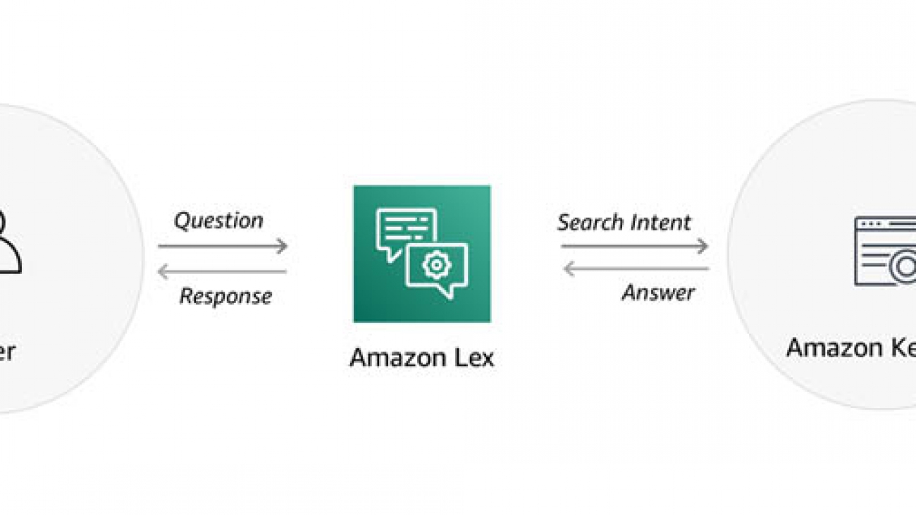
Integrate Amazon Kendra and Amazon Lex using a search intent
Customer service conversations typically revolve around one or more topics and contain related questions. Answering these questions seamlessly is essential for a good conversational experience. For example, as part of a car rental reservation, you have queries such as, “What’s the charge for an additional driver?” or, “Do you have car seats for kids?” Starting today, you can use a search intent in your Amazon Lex bots to integrate with Amazon Kendra, so your bots can surface answers from Kendra.
Amazon Kendra was recently made generally available to all AWS customers, with exciting new features. Amazon Kendra provides you with a highly accurate and easy-to-use enterprise search service powered by machine learning. It offers a more intuitive way to search—using natural language—and returns more accurate answers, so your end-users can discover information stored within your organization’s vast amount of content.
We previously described how you can add an AWS Lambda function in an Amazon Lex bot to integrate with Kendra. For more information, see Smarter FAQ bots with Amazon Kendra. With this approach, you need to write and maintain integration code, and any updates to the configuration require updating this code. Now you can can add a search intent to get the answers you’re looking for from FAQ documents. You simply define the search index parameters in the intent as part of the bot definition. The bot queries the Amazon Kendra search index during the interaction if the user input doesn’t match any of the other configured intents. The search query responses are populated with request attributes that the bot can use in its response. You don’t have to write any Lambda code. The integration is simple, and you can seamlessly deliver natural language answers from Amazon Kendra in your Amazon Lex conversations.
This post shows how you can integrate an Amazon Lex bot with Amazon Kendra using a search intent, so you can quickly build a bot to provide answers in a conversation. The following diagram illustrates this solution.
Building a Lex bot
We will use the same conversation from the previous post to model a bot conversation:
User: Where’s the IT Help Desk?
Agent: 2nd floor; room 201 (two rights after you get out of the elevators).
User: Can I come in at noon?
Agent: Sure. What’s the nature of your problem?
User: I have a cracked laptop screen.
Agent: For verification purposes, can I get the last four digits of your employee ID?
User: 1234.
Agent: Got it, we’ll see you then to take a look at your screen.
User: How long does it take to fix a screen?
Agent: Laptop screen repairs typically take 4 hours.
User: What do I need to bring with me for a screen repair?
Agent: For a laptop screen repair, please bring your employee badge, laptop, and VPN fob.
User: How do I access my documents while my laptop is being repaired?
Agent: You can use Amazon Workdocs to access your documents.
User: Can I use WorkDocs on my tablet?
Agent: Yes. Users can access Amazon WorkDocs using free applications for iPad, Kindle Fire, and Android tablets that you can download from iTunes, Amazon Appstore for Android, and Google Play. Users can also access Amazon WorkDocs using the web browser on any mobile device.
User: When does the help desk close?
Agent: Our hours are from 11 AM to 2 PM.
User: Is there a coffee shop nearby?
Agent: There is one on the third floor and it’s open from 8 AM to 4 PM daily.
The first step is to build an Amazon Lex bot with intents to book an appointment and check appointment status. The MakeAppointment intent elicits the information required to make an appointment, such as the date, time, employee ID, and the nature of the issue. The CheckAppointmentStatus intent provides the status of the appointment. When a user asks a question that the Lex bot can’t answer with these intents, it uses the built-in KendraSearchIntent intent to connect to Amazon Kendra to search for an appropriate answer.
Deploying the sample bot
To create the sample bot, complete the following steps. This creates an Amazon Lex bot called help_desk_bot and a Lambda fulfillment function called help_desk_bot_handler.
- Download the Amazon Lex definition and Lambda code.
- In the AWS Lambda console, choose Create function.
- Enter the function name
help_desk_bot_handler. - Choose the latest Python runtime (for example, Python 3.8).
- For Permissions, choose Create a new role with basic Lambda permissions.
- Choose Create function.
- Once your new Lambda function is available, in the Function code section, choose Actions, choose Upload a .zip file, choose Upload, and select the
help_desk_bot_lambda_handler.zipfile that you downloaded. - Choose Save.
- On the Amazon Lex console, choose Actions, and then Import.
- Choose the file
help_desk_bot.zipthat you downloaded, and choose Import. - On the Amazon Lex console, choose the bot
help_desk_bot. - For each of the intents, choose AWS Lambda function in the Fulfillment section, and select the
help_desk_bot_handlerfunction in the dropdown list. If you are prompted “You are about to give Amazon Lex permission to invoke your Lambda Function”, choose OK. - When all the intents are updated, choose Build.
At this point, you should have a working bot that is not yet connected to Amazon Kendra.
Creating an Amazon Kendra index
You’re now ready to create an Amazon Kendra index for your documents and FAQ. Complete the following steps:
- On the Amazon Kendra console, choose Launch Amazon Kendra.
- If you have existing Amazon Kendra indexes, choose Create index.
- For Index name, enter a name, such as
it-helpdesk. - For Description, enter an optional description, such as
IT Help Desk FAQs. - For IAM role, choose Create a new role to create a role to allow Amazon Kendra to access Amazon CloudWatch Logs.
- For Role name, enter a name, such as
cloudwatch-logs. Kendra will prefix the name withAmazonKendraand the AWS region. - Choose Next.

- For Provisioning editions, choose Developer edition.

- Choose Create.
Adding your FAQ content
While Amazon Kendra creates your new index, upload your content to an Amazon Simple Storage Service (Amazon S3) bucket.
- On the Amazon S3 console, create a new bucket, such as
kendra-it-helpdesk-docs-<your-account#>. - Keep the default settings and choose Create bucket.
- Download the following sample files and upload them to your new S3 bucket:
When the index creation is complete, you can add your FAQ content.
- On the Amazon Kendra console, choose your index, then choose FAQs, and Add FAQ.
- For FAQ name, enter a name, such as
it-helpdesk-faq. - For Description, enter an optional description, such as
FAQ for the IT Help Desk. - For S3, browse Amazon S3 to find your bucket, and choose help-desk-faq.csv.
- For IAM role, choose Create a new role to allow Amazon Kendra to access your S3 bucket.
- For Role name, enter a name, such as
s3-access. Kendra will prefix your role name withAmazonKendra-. - Choose Add.

- Stay on the page while Amazon Kendra creates your FAQ.
- When the FAQ is complete, choose Add FAQ to add another FAQ.
- For FAQ name, enter a name, such as
workdocs-faq. - For Description, enter a description, such as
FAQ for Amazon WorkDocsmobile and web access. - For S3, browse Amazon S3 to find your bucket, and choose workdocs-faq.csv.
- For IAM role, choose the same role you created in step 9.
- Choose Add.

After you create your FAQs, you can try some Kendra searches by choosing Search console. For example:
- When is the help desk open?
- When does the help desk close?
- Where is the help desk?
- Can I access WorkDocs from my phone?
Adding a search intent
Now that you have a working Amazon Kendra index, you need to add a search intent.
- On the Amazon Lex console, choose
help_desk_bot. - Under Intents, choose the + icon next to add an intent.
- Choose Search existing intents.
- Under Built-in intents, choose KendraSearchIntent.
- Enter a name for your intent, such as
help_desk_kendra_search. - Choose Add.
- Under Amazon Kendra query, choose the index you created (
it-helpdesk). - For IAM role, choose Add Amazon Kendra permissions.
- For Fulfillment, leave the default value Return parameters to client selected.

- For Response, choose Message, enter the following message value and choose + to add it:
((x-amz-lex:kendra-search-response-question_answer-answer-1)) - Choose Save intent.
- Choose Build.
The message value you used in step 10 is a request attribute, which is set automatically by the Amazon Kendra search intent. This response is only selected if Kendra surfaces an answer. For more information on request attributes, see the AMAZON.KendraSearchIntent documentation.
Your bot can now execute Amazon Kendra queries. You can test this on the Amazon Lex console. For example, you can try the sample conversation from the beginning of this post.
Deploying on a Slack channel
You can put this solution in a real chat environment, such as Slack, so that users can easily get information. To create a Slack channel association with your bot, complete the following steps:
- On the Amazon Lex console, choose Settings.
- Choose Publish.
- For Create an alias, enter an alias name, such as
test. - Choose Publish.
- When your alias is published, choose the Channels
- Under Channels, choose Slack.
- Enter a Channel Name, such as
slack_help_desk_bot. - For Channel Description, add an optional description.
- From the KMS Key drop-down menu, leave aws/lex selected.
- For Alias, choose
test. - Provide the Client Id, Client Secret, and Verification Token for your Slack application.

- Choose Activate to generate the OAuth URL and Postback URL.
Use the OAuth URL and Postback URL on the Slack application portal to complete the integration. For more information about setting up a Slack application and integrating with Amazon Lex, see Integrating an Amazon Lex Bot with Slack.
Conclusion
This post demonstrates how to integrate Amazon Lex and Amazon Kendra using a search intent. Amazon Kendra can extract specific answers from unstructured data. No pre-training is required; you simply point Amazon Kendra at your content, and it provides specific answers to natural language queries. For more information about incorporating these techniques into your bots, please see the AMAZON.KendraSearchIntent documentation.
About the authors
 Brian Yost is a Senior Consultant with the AWS Professional Services Conversational AI team. In his spare time, he enjoys mountain biking, home brewing, and tinkering with technology.
 As a Product Manager on the Amazon Lex team, Harshal Pimpalkhute spends his time trying to get machines to engage (nicely) with humans.
What jumps out in a photo changes the longer we look
What seizes your attention at first glance might change with a closer look. That elephant dressed in red wallpaper might initially grab your eye until your gaze moves to the woman on the living room couch and the surprising realization that the pair appear to be sharing a quiet moment together.
In a study being presented at the virtual Computer Vision and Pattern Recognition conference this week, researchers show that our attention moves in distinctive ways the longer we stare at an image, and that these viewing patterns can be replicated by artificial intelligence models. The work suggests immediate ways of improving how visual content is teased and eventually displayed online. For example, an automated cropping tool might zoom in on the elephant for a thumbnail preview or zoom out to include the intriguing details that become visible once a reader clicks on the story.
“In the real world, we look at the scenes around us and our attention also moves,” says Anelise Newman, the study’s co-lead author and a master’s student at MIT. “What captures our interest over time varies.” The study’s senior authors are Zoya Bylinskii PhD ’18, a research scientist at Adobe Research, and Aude Oliva, co-director of the MIT Quest for Intelligence and a senior research scientist at MIT’s Computer Science and Artificial Intelligence Laboratory.
What researchers know about saliency, and how humans perceive images, comes from experiments in which participants are shown pictures for a fixed period of time. But in the real world, human attention often shifts abruptly. To simulate this variability, the researchers used a crowdsourcing user interface called CodeCharts to show participants photos at three durations — half a second, 3 seconds, and 5 seconds — in a set of online experiments.
When the image disappeared, participants were asked to report where they had last looked by typing in a three-digit code on a gridded map corresponding to the image. In the end, the researchers were able to gather heat maps of where in a given image participants had collectively focused their gaze at different moments in time.
At the split-second interval, viewers focused on faces or a visually dominant animal or object. By 3 seconds, their gaze had shifted to action-oriented features, like a dog on a leash, an archery target, or an airborne frisbee. At 5 seconds, their gaze either shot back, boomerang-like, to the main subject, or it lingered on the suggestive details.
“We were surprised at just how consistent these viewing patterns were at different durations,” says the study’s other lead author, Camilo Fosco, a PhD student at MIT.
With real-world data in hand, the researchers next trained a deep learning model to predict the focal points of images it had never seen before, at different viewing durations. To reduce the size of their model, they included a recurrent module that works on compressed representations of the input image, mimicking the human gaze as it explores an image at varying durations. When tested, their model outperformed the state of the art at predicting saliency across viewing durations.
The model has potential applications for editing and rendering compressed images and even improving the accuracy of automated image captioning. In addition to guiding an editing tool to crop an image for shorter or longer viewing durations, it could prioritize which elements in a compressed image to render first for viewers. By clearing away the visual clutter in a scene, it could improve the overall accuracy of current photo-captioning techniques. It could also generate captions for images meant for split-second viewing only.
“The content that you consider most important depends on the time you have to look at it,” says Bylinskii. “If you see the full image at once, you may not have time to absorb it all.”
As more images and videos are shared online, the need for better tools to find and make sense of relevant content is growing. Research on human attention offers insights for technologists. Just as computers and camera-equipped mobile phones helped create the data overload, they are also giving researchers new platforms for studying human attention and designing better tools to help us cut through the noise.
In a related study accepted to the ACM Conference on Human Factors in Computing Systems, researchers outline the relative benefits of four web-based user interfaces, including CodeCharts, for gathering human attention data at scale. All four tools capture attention without relying on traditional eye-tracking hardware in a lab, either by collecting self-reported gaze data, as CodeCharts does, or by recording where subjects click their mouse or zoom in on an image.
“There’s no one-size-fits-all interface that works for all use cases, and our paper focuses on teasing apart these trade-offs,” says Newman, lead author of the study.
By making it faster and cheaper to gather human attention data, the platforms may help to generate new knowledge on human vision and cognition. “The more we learn about how humans see and understand the world, the more we can build these insights into our AI tools to make them more useful,” says Oliva.
Other authors of the CVPR paper are Pat Sukhum, Yun Bin Zhang, and Nanxuan Zhao. The research was supported by the Vannevar Bush Faculty Fellowship program, an Ignite grant from the SystemsThatLearn@CSAIL, and cloud computing services from MIT Quest.
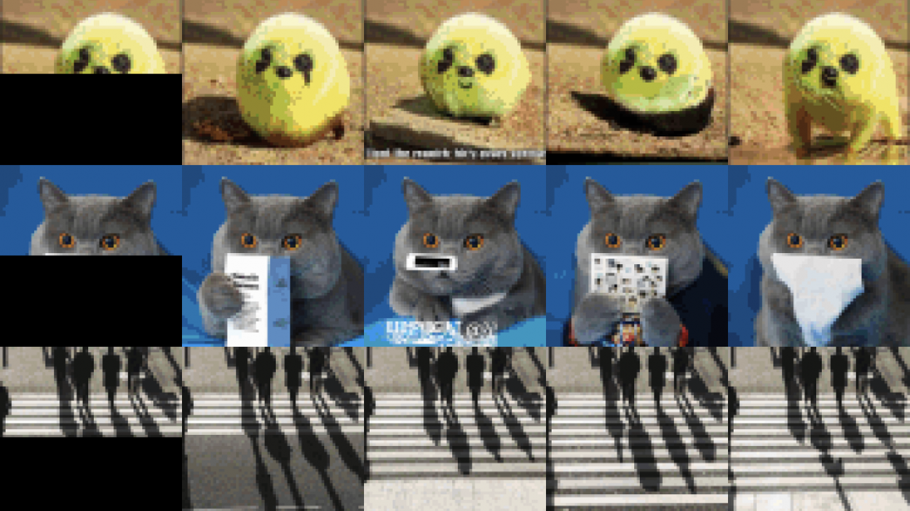
Image GPT

We find that, just as a large transformer model trained on language can generate coherent text, the same exact model trained on pixel sequences can generate coherent image completions and samples. By establishing a correlation between sample quality and image classification accuracy, we show that our best generative model also contains features competitive with top convolutional nets in the unsupervised setting.
Introduction
Unsupervised and self-supervised learning, or learning without human-labeled data, is a longstanding challenge of machine learning. Recently, it has seen incredible success in language, as transformer models like BERT, GPT-2, RoBERTa, T5, and other variants have achieved top performance on a wide array of language tasks. However, the same broad class of models has not been successful in producing strong features for image classification. Our work aims to understand and bridge this gap.
Transformer models like BERT and GPT-2 are domain agnostic, meaning that they can be directly applied to 1-D sequences of any form. When we train GPT-2 on images unrolled into long sequences of pixels, which we call iGPT, we find that the model appears to understand 2-D image characteristics such as object appearance and category. This is evidenced by the diverse range of coherent image samples it generates, even without the guidance of human provided labels. As further proof, features from the model achieve state-of-the-art performance on a number of classification datasets and near state-of-the-art unsupervised accuracy[1] on ImageNet.
| Evaluation | Dataset | Our Result | Best non-iGPT Result |
|---|---|---|---|
| Logistic regression on learned features (linear probe) | CIFAR-10 |
96.3
iGPT-L 32×32 w/ 1536 features |
95.3
SimCLR w/ 8192 features |
| CIFAR-100 |
82.8
iGPT-L 32×32 w/ 1536 features |
80.2
SimCLR w/ 8192 features |
|
| STL-10 |
95.5
iGPT-L 32×32 w/ 1536 features |
94.2
AMDIM w/ 8192 features |
|
| ImageNet |
72.0
iGPT-XLa 64×64 w/ 15360 features |
76.5
SimCLR w/ 8192 features |
|
| Full fine-tune | CIFAR-10 |
99.0
iGPT-L 32×32, trained on ImageNet |
99.0b
GPipe, trained on ImageNet |
| ImageNet 32×32 |
66.3
iGPT-L 32×32 |
70.2
Isometric Nets |
- We only show ImageNet linear probe accuracy for iGPT-XL since other experiments did not finish before we needed to transition to different supercomputing facilities.
- Bit-L, trained on JFT (300M images with 18K classes), achieved a result of 99.3.
To highlight the potential of generative sequence modeling as a general purpose unsupervised learning algorithm, we deliberately use the same transformer architecture as GPT-2 in language. As a consequence, we require significantly more compute in order to produce features competitive with those from top unsupervised convolutional nets. However, our results suggest that when faced with a new domain where the correct model priors are unknown, a large GPT-2 can learn excellent features without the need for domain-specific architectural design choices.
Completions
Favorites
Animals
Painted Landscapes
Sports
Architecture
ImageNet-R
Movie Posters
Famous Artworks
Popular Memes
Landscapes
Album Covers
Common English Words
US & State Flags
OpenAI Research Covers
OpenAI Pets
OpenAI Cooking
navigateleft
navigateright
Model Input
Completions right
Original


Model-generated completions of human-provided half-images. We sample the remaining halves with temperature 1 and without tricks like beam search or nucleus sampling. While we showcase our favorite completions in the first panel, we do not cherry-pick images or completions in all following panels.
Samples

Model-generated image samples. We sample these images with temperature 1 and without tricks like beam search or nucleus sampling. All of our samples are shown, with no cherry-picking. Nearly all generated images contain clearly recognizable objects.
From language GPT to image GPT
In language, unsupervised learning algorithms that rely on word prediction (like GPT-2 and BERT) have been extremely successful, achieving top performance on a wide array of language tasks. One possible reason for this success is that instances of downstream language tasks appear naturally in text: questions are often followed by answers (which could help with question-answering) and passages are often followed by summaries (which could help with summarization). In contrast, sequences of pixels do not clearly contain labels for the images they belong to.
Even without this explicit supervision, there is still a reason why GPT-2 on images might work: a sufficiently large transformer trained on next pixel prediction might eventually learn to generate diverse[2] samples with clearly recognizable objects. Once it learns to do so, an idea known as “Analysis by Synthesis”[3] suggests that the model will also know about object categories. Many early generative models were motivated by this idea, and more recently, BigBiGAN was an example which produced encouraging samples and features. In our work, we first show that better generative models achieve stronger classification performance. Then, through optimizing GPT-2 for generative capabilities, we achieve top-level classification performance in many settings, providing further evidence for analysis by synthesis.
Towards general unsupervised learning
Generative sequence modeling is a universal unsupervised learning algorithm: since all data types can be represented as sequences of bytes, a transformer can be directly applied to any data type without additional engineering. Our work tests the power of this generality by directly applying the architecture used to train GPT-2 on natural language to image generation. We deliberately chose to forgo hand coding any image specific knowledge in the form of convolutions or techniques like relative attention, sparse attention, and 2-D position embeddings.
As a consequence of its generality, our method requires significantly more compute to achieve competitive performance in the unsupervised setting. Indeed, contrastive methods are still the most computationally efficient methods for producing high quality features from images. However, in showing that an unsupervised transformer model is competitive with the best unsupervised convolutional nets, we provide evidence that it is possible to trade off hand coded domain knowledge for compute. In new domains, where there isn’t much knowledge to hand code, scaling compute seems an appropriate technique to test.
Approach
We train iGPT-S, iGPT-M, and iGPT-L, transformers containing 76M, 455M, and 1.4B parameters respectively, on ImageNet. We also train iGPT-XL[4], a 6.8 billion parameter transformer, on a mix of ImageNet and images from the web. Due to the large computational cost of modeling long sequences with dense attention, we train at the low resolutions of 32×32, 48×48, and 64×64.
While it is tempting to work at even lower resolutions to further reduce compute cost, prior work has demonstrated that human performance on image classification begins to drop rapidly below these sizes. Instead, motivated by early color display palettes, we create our own 9-bit color palette to represent pixels. Using this palette yields an input sequence length 3 times shorter than the standard (R, G, B) palette, while still encoding color faithfully.
Experimental results
There are two methods we use to assess model performance, both of which involve a downstream classification task. The first, which we refer to as a linear probe, uses the trained model to extract features[5] from the images in the downstream dataset, and then fits a logistic regression to the labels. The second method fine-tunes[6] the entire model on the downstream dataset.
Since next pixel prediction is not obviously relevant to image classification, features from the final layer may not be the most predictive of the object category. Our first result shows that feature quality is a sharply increasing, then mildly decreasing function of depth. This behavior suggests that a transformer generative model operates in two phases: in the first phase, each position gathers information from its surrounding context in order to build a contextualized image feature. In the second phase, this contextualized feature is used to solve the conditional next pixel prediction task. The observed two stage performance of our linear probes is reminiscent of another unsupervised neural net, the bottleneck autoencoder, which is manually designed so that features in the middle are used.
Feature quality depends heavily on the layer we choose to evaluate. In contrast with supervised models, the best features for these generative models lie in the middle of the network.
Our next result establishes the link between generative performance and feature quality. We find that both increasing the scale of our models and training for more iterations result in better generative performance, which directly translates into better feature quality.
Hover to see sample images up
Each line tracks a model throughout generative pre-training: the dotted markers denote checkpoints at steps 131K, 262K, 524K, and 1000K. The positive slopes suggest a link between improved generative performance and improved feature quality. Larger models also produce better features than smaller models. iGPT-XL is not included because it was trained on a different dataset.
When we evaluate our features using linear probes on CIFAR-10, CIFAR-100, and STL-10, we outperform features from all supervised and unsupervised transfer algorithms. Our results are also compelling in the full fine-tuning setting.
| Pre-trained on ImageNet | ||||
|---|---|---|---|---|
| Evaluation | Model | Accuracy | w/o labels | w/ labels |
| CIFAR-10 Linear Probe |
ResNet-152 | 94.0 | check | |
| SimCLR | 95.3 | check | ||
| iGPT-L 32×32 | 96.3 | check | ||
| CIFAR-100 Linear Probe |
ResNet-152 | 78.0 | check | |
| SimCLR | 80.2 | check | ||
| iGPT-L 32×32 | 82.8 | check | ||
| STL-10 Linear Probe |
AMDIM-L | 94.2 | check | |
| iGPT-L 32×32 | 95.5 | check | ||
| CIFAR-10 Fine-tune |
AutoAugment | 98.5 | ||
| SimCLR | 98.6 | check | ||
| GPipe | 99.0 | check | ||
| iGPT-L | 99.0 | check | ||
| CIFAR-100 Fine-tune |
iGPT-L | 88.5 | check | |
| SimCLR | 89.0 | check | ||
| AutoAugment | 89.3 | |||
| EfficientNet | 91.7 | check | ||
A comparison of linear probe and fine-tune accuracies between our models and top performing models which utilize either unsupervised or supervised ImageNet transfer. We also include AutoAugment, the best performing model trained end-to-end on CIFAR.
Given the resurgence of interest in unsupervised and self-supervised learning on ImageNet, we also evaluate the performance of our models using linear probes on ImageNet. This is an especially difficult setting, as we do not train at the standard ImageNet input resolution. Nevertheless, a linear probe on the 1536 features from the best layer of iGPT-L trained on 48×48 images yields 65.2% top-1 accuracy, outperforming AlexNet.
Contrastive methods typically report their best results on 8192 features, so we would ideally evaluate iGPT with an embedding dimension of 8192 for comparison. However, training such a model is prohibitively expensive, so we instead concatenate features from multiple layers as an approximation. Unfortunately, our features tend to be correlated across layers, so we need more of them to be competitive. Taking 15360 features from 5 layers in iGPT-XL yields 72.0% top-1 accuracy, outperforming AMDIM, MoCo, and CPC v2, but still underperforming SimCLR by a decent margin.
| Method | Input Resolution | Features | Parameters | Accuracy |
|---|---|---|---|---|
| Rotation | original | 8192 | 86M | 55.4 |
| iGPT-L | 32×32 | 1536 | 1362M | 60.3 |
| BigBiGAN | original | 16384 | 86M | 61.3 |
| iGPT-L | 48×48 | 1536 | 1362M | 65.2 |
| AMDIM | original | 8192 | 626M | 68.1 |
| MoCo | original | 8192 | 375M | 68.6 |
| iGPT-XL | 64×64 | 3072 | 6801M | 68.7 |
| SimCLR | original | 2048 | 24M | 69.3 |
| CPC v2 | original | 4096 | 303M | 71.5 |
| iGPT-XL | 64×64 | 3072 x 5 | 6801M | 72.0 |
| SimCLR | original | 8192 | 375M | 76.5 |
A comparison of linear probe accuracies between our models and state-of-the-art self-supervised models. We achieve competitive performance while training at much lower input resolutions, though our method requires more parameters and compute.
Because masked language models like BERT have outperformed generative models on most language tasks, we also evaluate the performance of BERT on our image models. Instead of training our model to predict the next pixel given all preceding pixels, we mask out 15% of the pixels and train our model to predict them from the unmasked ones. We find that though linear probe performance on BERT models is significantly worse, they excel during fine-tuning:
CIFAR-10
ImageNet
Comparison of generative pre-training with BERT pre-training using iGPT-L at an input resolution of 322 × 3. Bold colors show the performance boost from ensembling BERT masks. We see that generative models produce much better features than BERT models after pre-training, but BERT models catch up after fine-tuning.
While unsupervised learning promises excellent features without the need for human-labeled data, significant recent progress has been made under the more forgiving framework of semi-supervised learning, which allows for limited amounts of human-labeled data. Successful semi-supervised methods often rely on clever techniques such as consistency regularization, data augmentation, or pseudo-labeling, and purely generative-based approaches have not been competitive for years. We evaluate iGPT-L[7] on a competitive benchmark for this sub-field and find that a simple linear probe on features from non-augmented images outperforms Mean Teacher and MixMatch, though it underperforms FixMatch.
| Model | 40 labels | 250 labels | 4000 labels |
|---|---|---|---|
| Improved GAN | — | — | 81.4 ± 2.3 |
| Mean Teacher | — | 67.7 ± 2.3 | 90.8 ± 0.2 |
| MixMatch | 52.5 ± 11.5 | 89.0 ± 0.9 | 93.6 ± 0.1 |
| iGPT-L | 73.2 ± 01.5 | 87.6 ± 0.6 | 94.3 ± 0.1 |
| UDA | 71.0 ± 05.9 | 91.2 ± 1.1 | 95.1 ± 0.2 |
| FixMatch RA | 86.2 ± 03.4 | 94.9 ± 0.7 | 95.7 ± 0.1 |
| FixMatch CTA | 88.6 ± 03.4 | 94.9 ± 0.3 | 95.7 ± 0.2 |
A comparison of performance on low-data CIFAR-10. By leveraging many unlabeled ImageNet images, iGPT-L is able to outperform methods such as Mean Teacher and MixMatch but still underperforms the state of the art methods. Our approach to semi-supervised learning is very simple since we only fit a logistic regression classifier on iGPT-L’s features without any data augmentation or fine-tuning—a significant difference from specially designed semi-supervised approaches.
Limitations
While we have shown that iGPT is capable of learning powerful image features, there are still significant limitations to our approach. Because we use the generic sequence transformer used for GPT-2 in language, our method requires large amounts of compute: iGPT-L was trained for roughly 2500 V100-days while a similarly performing MoCo model can be trained in roughly 70 V100-days.
Relatedly, we model low resolution inputs using a transformer, while most self-supervised results use convolutional-based encoders which can easily consume inputs at high resolution. A new architecture, such as a domain-agnostic multiscale transformer, might be needed to scale further. Given these limitations, our work primarily serves as a proof-of-concept demonstration of the ability of large transformer-based language models to learn excellent unsupervised representations in novel domains, without the need for hardcoded domain knowledge. However, the significant resource cost to train these models and the greater accuracy of convolutional neural-network based methods precludes these representations from practical real-world applications in the vision domain.
Finally, generative models can exhibit biases that are a consequence of the data they’ve been trained on. Many of these biases are useful, like assuming that a combination of brown and green pixels represents a branch covered in leaves, then using this bias to continue the image. But some of these biases will be harmful, when considered through a lens of fairness and representation. For instance, if the model develops a visual notion of a scientist that skews male, then it might consistently complete images of scientists with male-presenting people, rather than a mix of genders. We expect that developers will need to pay increasing attention to the data that they feed into their systems and to better understand how it relates to biases in trained models.
Conclusion
We have shown that by trading off 2-D knowledge for scale and by choosing predictive features from the middle of the network, a sequence transformer can be competitive with top convolutional nets for unsupervised image classification. Notably, we achieved our results by directly applying the GPT-2 language model to image generation. Our results suggest that due to its simplicity and generality, a sequence transformer given sufficient compute might ultimately be an effective way to learn excellent features in many domains.
If you’re excited to work with us on this area of research, we’re hiring!
OpenAI

From singing to musical scores: Estimating pitch with SPICE and Tensorflow Hub
Posted by Luiz Gustavo Martins, Beat Gfeller and Christian Frank
Pitch is an attribute of musical tones (along with duration, intensity and timbre) that allows you to describe a note as “high” or “low”. Pitch is quantified by frequency, measured in Hertz (Hz), where one Hz corresponds to one cycle per second. The higher the frequency, the higher the note.
Pitch detection is an interesting challenge. Historically, for a machine to understand pitch, it would need to rely on complex hand-crafted signal-processing algorithms to measure the frequency of a note, in particular to separate the relevant frequency from background noise and backing instruments. Today, we can do that with machine learning, more specifically with the SPICE model (SPICE: Self-Supervised Pitch Estimation).
SPICE is a pretrained model that can recognize the fundamental pitch from mixed audio recordings (including noise and backing instruments). The model is also available to use on the web with TensorFlow.js and on mobile devices with TensorFlow Lite.
In this tutorial, we’ll walk you through using SPICE to extract the pitch from short musical clips. First we will load the audio file and process it. Then we will use machine learning to solve this problem (and you’ll notice how easy it is with TensorFlow Hub). Finally, we will do some post-processing and some cool visualization. You can follow along with this Colab notebook.
Loading the audio file
The model expects raw audio samples as input. To help you with this, we’ve shown four methods you can use to import your input wav file to the colab:
- Record a short clip of yourself singing directly in Colab
- Upload a recording from your computer
- Download a file from your Google Drive
- Download a file from a URL
You can choose any one of these methods. Recording yourself singing directly in Colab is the easiest one to try, and the most fun.
Audio can be recorded in many formats (for example, you might record using an Android app, or on a desktop computer, or on the browser), converting your audio into the exact format the model expects can be challenging. To help you with that, there’s a helper function convert_audio_for_model to convert your wav file to the correct format of one audio channel at 16khz sampling rate.
For the rest of this post, we will use this file:
Preparing the audio data
Now that we have loaded the audio, we can visualize it using a spectrogram, which shows frequencies over time. Here, we use a logarithmic frequency scale, to make the singing more clearly visible (note that this step is not required to run the model, it is just for visualization).
 |
| Note: this graph was created using Librosa lib. You can find more information here. |
We need one last conversion. The input must be normalized to floats between -1 and 1. In a previous step we converted the audio to be in 16 bit format (using the helper function convert_audio_for_model). To normalize it, we just need to divide all the values by 216 or in our code, MAX_ABS_INT16:
audio_samples = audio_samples / float(MAX_ABS_INT16)Executing the model
Loading a model from TensorFlow Hub is simple. You just use the load method with the model’s URL.
model = hub.load("https://tfhub.dev/google/spice/2")Note: An interesting detail here is that all the model urls from Hub can be used for download and also to read the documentation, so if you point your browser to that link, you can read documentation on how to use the model and learn more about how it was trained.
Now we can use the model loaded from TensorFlow Hub by passing our normalized audio samples:
output = model.signatures["serving_default"](tf.constant(audio_samples, tf.float32))

pitch_outputs = output["pitch"]
uncertainty_outputs = output["uncertainty"]
At this point we have the pitch estimation and the uncertainty (per pitch detected). Converting uncertainty to confidence (confidence_outputs = 1.0 - uncertainty_outputs), we can get a good understanding of the results:  As we can see, for some predictions (especially where no singing voice is present), the confidence is very low. Let’s only keep the predictions with high confidence by removing the results where the confidence was below 0.9.
 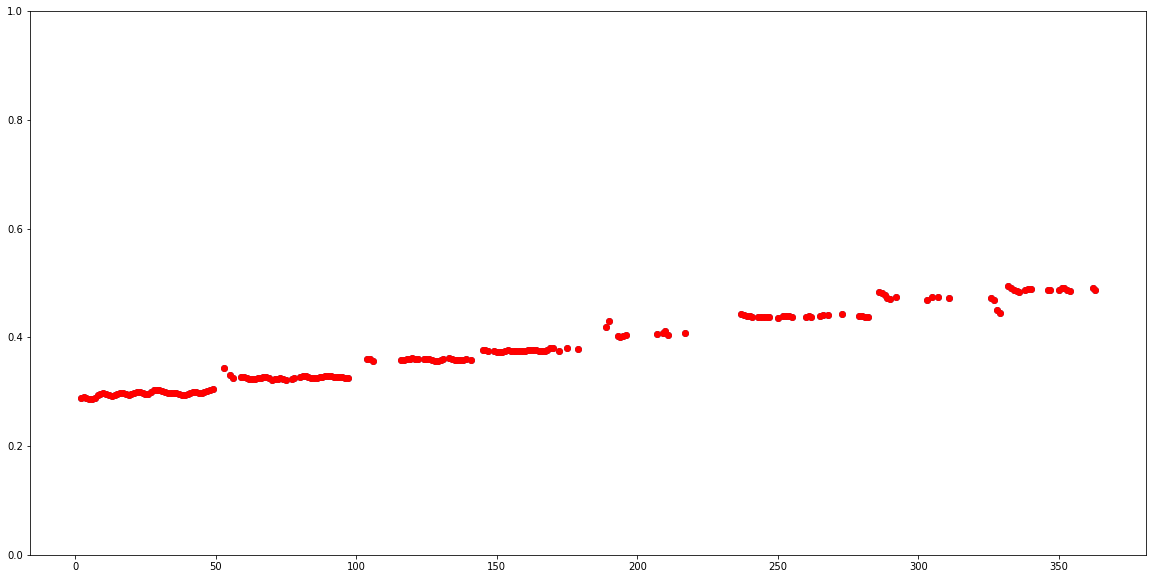 To confirm that the model is working correctly, let’s convert pitch from the [0.0, 1.0] range to absolute values in Hz. To do this conversion we can use the function present in the Colab notebook:
def output2hz(pitch_output):
  # Constants taken from https://tfhub.dev/google/spice/2
  PT_OFFSET = 25.58
  PT_SLOPE = 63.07
  FMIN = 10.0;
  BINS_PER_OCTAVE = 12.0;
  cqt_bin = pitch_output * PT_SLOPE + PT_OFFSET;
  return FMIN * 2.0 ** (1.0 * cqt_bin / BINS_PER_OCTAVE)

confident_pitch_values_hz = [ output2hz(p) for p in confident_pitch_outputs_y ]
If we plot these values over the spectrogram we can see how well the predictions match the dominant pitch, that can be seen as the stronger lines in the spectrogram: 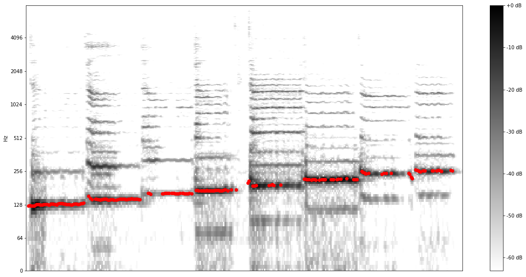 Success! We managed to extract the relevant pitch from the singer’s voice.
Note that for this particular example, a spectrogram-based heuristic for extracting pitch may have worked as well. In general, ML-based models perform better than hand-crafted signal processing methods in particular when background noise and backing instruments are present in the audio. For a comparison of SPICE with a spectrogram-based algorithm (SWIPE) see here.
Converting to musical notes
To make the pitch information more useful, we can also find the notes that each pitch represents. To do that we will apply some math to convert frequency to notes. One important observation is that, in contrast to the inferred pitch values, the converted notes are quantized as this conversion involves rounding (the function hz2offset in the notebook, uses some math for which you can find a good explanation here). In addition, we also need to group the predictions together in time, to obtain longer sustained notes instead of a sequence of equal ones. This temporal quantization is not easy, and our notebook just implements some heuristics which won’t produce perfect scores in general. It does work for sequences of notes with equal durations though, as in our example.
We start by adding rests (no singing intervals) based on the predictions that had low confidence. The next step is more challenging. When a person sings freely, the melody may have an offset to the absolute pitch values that notes can represent. Hence, to convert predictions to notes, one needs to correct for this possible offset.
After calculating the offsets and trying different speeds (how many predictions make an eighth) we end up with these rendered notes:  We can also export the converted notes to a MIDI file using music21:
converted_audio_file_as_midi = converted_audio_file[:-4] + '.mid'
fp = sc.write('midi', fp=converted_audio_file_as_midi)
What’s next?
With TensorFlow Hub you can easily find great models, like SPICE and many others, to help you solve your machine learning challenges. Keep exploring the model, play with the colab and maybe try building something similar to FreddieMeter, but with your favorite singer!
We are eager to know what you can come up with. Share your ideas with us on social media adding the #TFHub to your post.
Acknowledgements
This blog post is based on work by Beat Gfeller, Christian Frank, Dominik Roblek, Matt Sharifi, Marco Tagliasacchi and Mihajlo Velimirović on SPICE: Self-Supervised Pitch Estimation. Thanks also to Polong Lin for reviewing and suggesting great ideas and to Jaesung Chung for supporting the creation of the TF Lite version of the model.Read More
2019 Amazon Research Awards recipients announcement
Earlier this year, Amazon notified grant applicants who were recipients of the 2019 Amazon Research Awards.Read More
Michael J. Black awarded CVPR “test of time” honor
Black, a distinguished Amazon scholar, has been awarded the Longuet-Higgins Prize. Award recognizes paper that has made a significant impact in computer vision research field.Read More
Detecting and visualizing telecom network outages from tweets with Amazon Comprehend
In today’s world, social media has become a place where customers share their experiences with services that they consume. Every telecom provider wants to have the ability to understand their customer pain points as soon as possible and to do this carriers frequently establish a social media team within their NOC (network operation center). This team manually reviews social media messages, such as tweets, trying to identify patterns of customer complaints or issues that might suggest that there is a specific problem in the carrier’s network .
Unhappy customers are more likely to change provider, so operators look to improve their customers’ experience and proactively approach dissatisfied customers who are reporting issues with their services .
Of course, social media operates at a vast scale and our telecom customers are telling us that trying to uncover customer issues from social media data manually is extremely challenging.
This post shows how to classify tweets in real time so telecom companies can identify outages and proactively engage with customers by using Amazon Comprehend custom multi-class classification.
Solution overview
Telecom customers not only post about outages on social media, but also comment on the service they get or compare the company to a competitor.
Your company can benefit from targeting those types of tweets separately. One option is customer feedback, in which care agents respond to the customer. For outages, you need to collect information and open a ticket in an external system so an engineer can specify the problem.
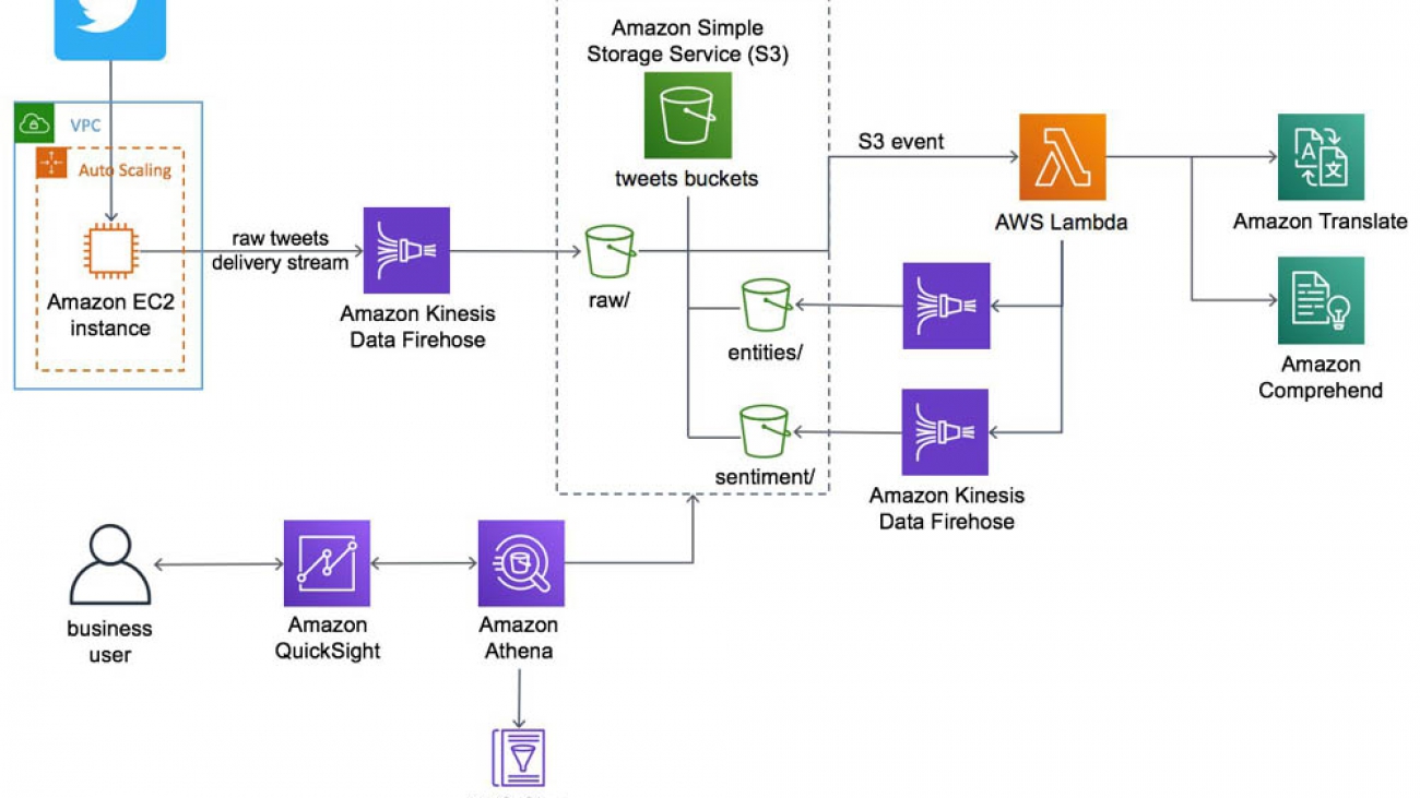
The solution for this post extends the AI-Driven Social Media Dashboard solution. The following diagram illustrates the solution architecture.

AI-Driven Social Media Dashboard Solutions Implementation architecture
This solution deploys an Amazon Elastic Compute Cloud (Amazon EC2) instance running in an Amazon Virtual Private Cloud (Amazon VPC) that ingests tweets from Twitter. An Amazon Kinesis Data Firehose delivery stream loads the streaming tweets into the raw prefix in the solution’s Amazon Simple Storage Service (Amazon S3) bucket. Amazon S3 invokes an AWS Lambda function to analyze the raw tweets using Amazon Translate to translate non-English tweets into English, and Amazon Comprehend to use natural-language-processing (NLP) to perform entity extraction and sentiment analysis.
A second Kinesis Data Firehose delivery stream loads the translated tweets and sentiment values into the sentiment prefix in the Amazon S3 bucket. A third delivery stream loads entities in the entities prefix using in the Amazon S3 bucket.
The solution also deploys a data lake that includes AWS Glue for data transformation, Amazon Athena for data analysis, and Amazon QuickSight for data visualization. AWS Glue Data Catalog contains a logical database which is used to organize the tables for the data on Amazon S3. Athena uses these table definitions to query the data stored on Amazon S3 and return the information to an Amazon QuickSight dashboard.
You can extend this solution by building Amazon Comprehend custom classification to detect outages, customer feedback, and comparisons to competitors.
Creating the dataset
The solution uses raw data from tweets. In the original solution, you deploy an AWS CloudFormation template that defines a comma-delimited list of terms for the solution to monitor. As an example, this post focuses on tweets that contain the word “BT” (BT Group in the UK), but equally this could be any network provider.
To get started, launch the AI-driven Social Media Dashboard solution. On the Specify Stack Details page, replace the default TwitterTermList with your terms. For this example, 'BT','bt'. After you click on Create Stack, wait 15 minutes for the deployment to complete. You will now begin capturing tweets.
For more information about available attributes and data types, see Appendix B: Auto-generated Data Model.
The tweet data is stored in Amazon Simple Storage Service (Amazon S3), which you can query with Amazon Athena. The following screenshot shows an example query.
SELECT id,text FROM "ai_driven_social_media_dashboard"."tweets" limit 10;
Because you captured every tweet that contains the keyword BT or bt, you have a lot of tweets that aren’t referring to British Telecom; for example, tweets that misspell the word “but.”
Additionally, the tweets in your dataset are global, but for this post, you want to focus on the United Kingdom, so the tweets are even more likely to refer to British Telecom (and therefore your dataset is more accurate). You can modify this solution for use cases in other countries, for example, defining the keyword as KPN and narrowing the dataset to focus only on the Netherlands.
In the existing solution, the coordinates and geo types look relevant, but those usually aren’t populated—tweets don’t include the poster’s location by default due to privacy requirements, unless the user allows it.
The user type contains relevant user data that comes from the user profile. You can use the location data from the user profile to narrow down tweets to your target country or region.
To look at the user type, you can use the Athena CREATE TABLE AS SELECT (CTAS) query. For more information, see Creating a Table from Query Results (CTAS). The following screenshot shows the Create table from query option in the Create drop-down menu.
SELECT text,user.location from tweets
You can create a table that consists of the tweet text and the user location, which gives you the ability to look only at tweets that originated in the UK. The following screenshot shows the query results.
SELECT * FROM "ai_driven_social_media_dashboard"."location_text_02"
WHERE location like '%UK%' or location like '%England%' or location like '%Scotland%' or location like '%Wales%'
Now that you have a dataset with your target location and tweet keywords, you can train your custom classifier.
Amazon Comprehend custom classification
You train your model in multi-class mode. For this post, you label three different classes:
- Outage – People who are experiencing or reporting an outage in their provider network
- Customer feedback – Feedback regarding the service they have received from the provider
- Competition – Tweets about the competition and the provider itself
You can export the dataset from Athena and train it to use the custom classifier.
You first look at the dataset and start labeling the different tweets. Because you have a large number of tweets, it can take manual effort and perhaps several hours to review the data and label it. We recommend that you train the model with at least 50 documents per label.
In the dataset, customers reported an outage, which resulted in 71 documents with the outage label. Competition and customer feedback had under 50 labels.
After you gather sufficient data, you can always improve your accuracy by training a new model.
The following screenshot shows some of the entries in the final training CSV file.

As a future enhancement to remove the manual effort of labeling tweets, you can automate the process with Amazon SageMaker Ground Truth. Ground Truth offers easy access to labelers through Amazon Mechanical Turk and provides built-in workflows and interfaces for common labeling tasks.
When the labeling work is complete, upload the CSV file to your S3 bucket.

Now that the training data is in Amazon S3, you can train your custom classifier. Complete the following steps:
- On the Amazon Comprehend console, choose Custom classification.
- Choose Train classifier.

- For Name, enter a name for your classifier; for example,
TweetsBT. - For Classifier mode, select Using multi-class mode.
- For S3 location, enter the location of your CSV file.

- Choose Train classifier.
The status of the classifier changes from Submitted to Training. When the job is finished, the status changes to Trained.
After you train the custom classifier, you can analyze documents in either asynchronous or synchronous operations. You can analyze a large number of documents at the same time by using the asynchronous operation. The resulting analysis returns in a separate file. When you use the synchronous operation, you can only analyze a single document, but you can get results in real time.
For this use case, you want to analyze tweets in real time. When a tweet lands in Amazon S3 via Amazon Kinesis Data Firehose, it triggers an AWS Lambda function. The function triggers the custom classifier endpoint to run an analysis on the tweet and determine if it’s in regards to an outage, customer feedback, or referring to a competitor.
Testing the training data
After you train the model, Amazon Comprehend uses approximately 10% of the training documents to test the custom classifier model. Testing the model provides you with metrics that you can use to determine if the model is trained well enough for your purposes. These metrics are displayed in the Classifier performance section of the Classifier details page on the Amazon Comprehend console. See the following screenshot.

They’re also returned in the Metrics fields returned by the DescribeDocumentClassifier operation.
Creating an endpoint
To create an endpoint, complete the following steps:
- On the Amazon Comprehend console, choose Custom classification.
- From the Actions drop-down menu, choose Create endpoint.

- For Endpoint name, enter a name; for example,
BTtweetsEndpoint. - For Inference units¸ enter the number to assign to an endpoint.
Each unit represents a throughput of 100 characters per second for up to two documents per second. You can assign up to 10 inference units per endpoint. This post assigns 1.
- Choose Create endpoint.

When the endpoint is ready, the status changes to Ready.

Triggering the endpoint and customizing the existing Lambda function
You can use the existing Lambda function from the original solution and extend it to do the following:
- Trigger the Amazon Comprehend custom classifier endpoint per tweet
- Determine which class has the highest confidence score
- Create an additional Firehose delivery stream so the results land back in Amazon S3
For more information about the original Lambda function, see the GitHub repo.
To make the necessary changes to the function, complete the following steps:
- On the Lambda console, select the function that contains the string Tweet-SocialMediaAnalyticsLambda.

Before you start adding code, make sure you understand how the function reads the tweets coming in, calls the Amazon Comprehend API, and stores the responses on a Firehose delivery stream so it writes the data to Amazon S3.
- Call the custom classifier endpoint (see the following code example).
The first two calls use the API on the tweet text to detect sentiment and entities; those both come out-of-the-box with the officinal solution.
The following code uses the ClassifyDocument API:
 sentiment_response = comprehend.detect_sentiment(
                    Text=comprehend_text,
                    LanguageCode='en'
                )
            #print(sentiment_response)

            entities_response = comprehend.detect_entities(
                    Text=comprehend_text,
                    LanguageCode='en'
                )

            #we will create a 'custom_response' using the ClassifyDocument API call
            custom_response = comprehend.classify_document(
                     #point to the relevant Custom classifier endpoint ARN
                     EndpointArn= "arn:aws:comprehend:us-east-1:12xxxxxxx91:document-classifier-endpoint/BTtweets-endpoint",
                     #this is where we use comprehend_text which is the original tweet text
                     Text=comprehend_text

                )
The following code is the returned result:
{"File": "all_tweets.csv", "Line": "23", "Classes": [{"Name": "outage", "Score": 0.9985}, {"Name": "Competition", "Score": 0.0005}, {"Name": "Customer feedback", "Score": 0.0005}]}You now need to iterate over to the array, which contains the classes and confidence scores. For more information, see DocumentClass.
Because you’re using the multi-class approach, you can pick the class with the highest score and add some simple code that iterates over the array and takes the biggest score and class.
You also take tweet[‘id’] because you can join it with the other tables that the solution generates to relate the results to the original tweet.
- Enter the following code:
score=0
        for classs in custom_response['Classes']:
         if score<classs['Score']:
             score=classs['Score']
             custom_record = {

                'tweetid': tweet['id'],
                'classname':classs['Name'],
                'classscore':classs['Score']
             }
After you create the custom_record, you can decide if you want to define a certain threshold for your class score (the level of confidence for the results you want to store in Amazon S3). For this use case, you choose to only define classes with a confidence score of at least 70%.
To put the result on a Firehose delivery stream (which you need to create in advance), use the PutRecord API. See the following code:
if custom_record['classscore']>0.7:
         print('we are in')
         response = firehose.put_record(
                        DeliveryStreamName=os.environ['CUSTOM_STREAM'],
                        Record={
                            'Data': json.dumps(custom_record) + 'n'
                        }
                    )
You now have a dataset in Amazon S3 based on your Amazon Comprehend custom classifier output.
Exploring the output
You can now explore the output from your custom classifier in Athena. Complete the following steps:
- On the Athena console, run a
SELECTquery to see the following:- tweetid – You can use this to join the original tweet table to get the tweet text and additional attributes.
- classname – This is the class that the custom classifier identified the tweet as with the highest level of confidence.
- classscore – This is the level of confidence.
- Stream partitions – These help you know the time when the data was written to Amazon S3:
Partition_0(month)Partition_1(day)Partition_2(hour)
The following screenshot shows your query results.
SELECT * FROM "ai_driven_social_media_dashboard"."custom2020" where classscore>0.7 limit 10;

- Join your table using the
tweetidwith the following:- The original tweet table to get the actual tweet text.
- A sentiment table that Amazon Comprehend generated in the original solution.
The following screenshot shows your results. One of the tweets contains negative feedback, and other tweets identify potential outages.
SELECT classname,classscore,tweets.text,sentiment FROM "ai_driven_social_media_dashboard"."custom2020"
left outer join tweets on custom2020.tweetid=tweets.id
left outer join tweet_sentiments on custom2020.tweetid=tweet_sentiments.tweetid
where classscore>0.7
limit 10;
Preparing the data for visualization
To prepare the data for visualization, first create a timestamp field by concatenating the partition fields.
You can use timestamp field for various visualizations, such as outages in a certain period or customer feedback on a specific day. To do so, use AWS Glue notebooks and write a piece of code in PySpark.
You can use the PySpark code to not only prepare your data but also transform the data from CSV to Apache Parquet format. For more information, see the GitHub repo.
You should now have a new dataset that contains a timestamp field in Parquet format, which is more efficient and cost-effective to query.
For this use case, you can determine the outages reported on a map using geospacial charts in Amazon QuickSight. To get the location of the tweet, you can use the following:
- Longitude and latitude coordinates in the original
tweetsdataset. Unfortunately, coordinates aren’t usually present due to privacy defaults. - Amazon Comprehend
entitydataset, which can identify locations as entities within the tweet text.
For this use case, you can create a new dataset combining the tweets, custom2020 (your new dataset based on the custom classifier output, and tweetsEntities datasets.
The following screenshot shows the query results, which returned tweets with locations that also identify outages.
SELECT distinct classname,final,text,entity FROM "ai_driven_social_media_dashb
oard"."custom2020"."quicksight_with_lat_lang"
where type='LOCATION' and classname='outage'
order by final asc 
You have successfully identified outages in a specific window and determined their location.
To get the geolocation of a specific location, you could choose from a variety of publicly available datasets to upload to Amazon S3 and join with your data. This post uses the World Cities Database, which has a free option. You can join it with your existing data to get the location coordinates.
Visualizing outage locations in Amazon QuickSight
To visualize your outage locations in Amazon QuickSight, complete the following steps:
- To add the dataset you created in Athena, on the Amazon QuickSight console, choose Manage data.
- Choose New dataset.
- Choose Athena.
- Select your database or table.

- Choose Save & Visualize.
- Under Visual types, choose the Points on map
- Drag the lng and lat fields to the field wells.
The following screenshot shows the outages on a UK map.

To see the text of a specific tweet, hover over one of the dots on the map.

You have many different options when analyzing your data and can further enhance this solution. For example, you can enrich your dataset with potential contributors and drill down on a specific outage location for more details.
Conclusion
We have now the ability to detect outages which customers are reporting upon, we can also leverage the solution to look on customer feedback and competition. We are now able to identify key trends on the social media at scale. In the blog post we have showed an example which is relevant for telecom companies, but this solution can be customized and leveraged by every company that has customers using the social media.
In the near feature, we would like to extend this solution, and create an end to end flow , where the customer reporting an outage ,will automatically receive a reply in tweeter from an Amazon Lex chat bot, which can ask for more information from the customer who complained via a secured channel and send this info to a call center agent via an integration with Amazon Connect or create a ticket in an external ticket system for an engineer to work on the problem .
Give the solution a try, see if you can extend it further, and share your feedback and questions in the comments.
About the Author
 Guy Ben-Baruch is a Senior solution architect in the news & communications team in AWS UKIR. Since Guy joined AWS in March 2016, he has worked closely with enterprise customers, focusing on the telecom vertical, supporting their digital transformation and their cloud adoption. Outside of work, Guy likes doing BBQ and playing football with his kids in the park when the British weather allows it.
Amazon Polly launches a child US English NTTS voice
Amazon Polly turns text into lifelike speech, allowing you to create voice-enabled applications. We’re excited to announce the general availability of a new US English child voice—Kevin. Kevin’s voice was developed using the latest Neural Text-to-Speech (NTTS) technology, making it sound natural and human-like. This voice imitates the voice of a male child. Have a listen to the Kevin voice:
Kevin sample 1
| Listen now Voiced by Amazon Polly |
Kevin sample 2
| Listen now Voiced by Amazon Polly |
Amazon Polly has 14 neural voices to choose from:
- US English (en-US): Ivy, Joey, Justin, Kendra, Kevin, Kimberly, Joanna, Matthew, Salli
- British English (en-GB): Amy, Brian, Emma
- Brazilian Portuguese (pt-BR): Camila
- US Spanish (es-US): Lupe
Neural voices are supported in the following Regions:
- US East (N. Virginia)
- US West (Oregon)
- Asia Pacific (Sydney)
- EU (Ireland)
For the full list of text-to-speech voices, see Voices in Amazon Polly.
Our customers are using Amazon Polly voices to build new categories of speech-enabled products, including (but not limited to) voicing news content, games, eLearning platforms, telephony applications, accessibility applications, and Internet of Things (IoT). Amazon Polly voices are high quality, cost-effective, and ensure fast responses, which makes it a viable option for low-latency use cases. Amazon Polly also supports SSML tags, which give you additional control over speech output.
For more information, see What Is Amazon Polly? and log in to the Amazon Polly console to try it out!
About the Author
 Ankit Dhawan is a Senior Product Manager for Amazon Polly, technology enthusiast, and huge Liverpool FC fan. When not working on delighting our customers, you will find him exploring the Pacific Northwest with his wife and dog. He is an eternal optimist, and loves reading biographies and playing poker. You can indulge him in a conversation on technology, entrepreneurship, or soccer any time of the day.