Watch the fireside chat featuring Charlie Bell, senior vice president of Amazon Web Services.Read More
Bringing the predictive power of artificial intelligence to health care
An important aspect of treating patients with conditions like diabetes and heart disease is helping them stay healthy outside of the hospital — before they to return to the doctor’s office with further complications.
But reaching the most vulnerable patients at the right time often has more to do with probabilities than clinical assessments. Artificial intelligence (AI) has the potential to help clinicians tackle these types of problems, by analyzing large datasets to identify the patients that would benefit most from preventative measures. However, leveraging AI has often required health care organizations to hire their own data scientists or settle for one-size-fits-all solutions that aren’t optimized for their patients.
Now the startup ClosedLoop.ai is helping health care organizations tap into the power of AI with a flexible analytics solution that lets hospitals quickly plug their data into machine learning models and get actionable results.
The platform is being used to help hospitals determine which patients are most likely to miss appointments, acquire infections like sepsis, benefit from periodic check ups, and more. Health insurers, in turn, are using ClosedLoop to make population-level predictions around things like patient readmissions and the onset or progression of chronic diseases.
“We built a health care data science platform that can take in whatever data an organization has, quickly build models that are specific to [their patients], and deploy those models,” says ClosedLoop co-founder and Chief Technology Officer Dave DeCaprio ’94. “Being able to take somebody’s data the way it lives in their system and convert that into a model that can be readily used is still a problem that requires a lot of [health care] domain knowledge, and that’s a lot of what we bring to the table.”
In light of the Covid-19 pandemic, ClosedLoop has also created a model that helps organizations identify the most vulnerable people in their region and prepare for patient surges. The open source tool, called the C-19 Index, has been used to connect high-risk patients with local resources and helped health care systems create risk scores for tens of millions of people overall.
The index is just the latest way that ClosedLoop is accelerating the health care industry’s adoption of AI to improve patient health, a goal DeCaprio has worked toward for the better part of his career.
Designing a strategy
After working as a software engineer for several private companies through the internet boom of the early 2000s, DeCaprio was looking to make a career change when he came across a project focused on genome annotation at the Broad Institute of MIT and Harvard.
The project was DeCaprio’s first professional exposure to the power of artificial intelligence. It blossomed into a six year stint at the Broad, after which he continued exploring the intersection of big data and health care.
“After a year in health care, I realized it was going to be really hard to do anything else,” DeCaprio says. “I’m not going to be able to get excited about selling ads on the internet or anything like that. Once you start dealing with human health, that other stuff just feels insignificant.”
In the course of his work, DeCaprio began noticing problems with the ways machine learning and other statistical techniques were making their way into health care, notably in the fact that predictive models were being applied without regard for hospitals’ patient populations.
“Someone would say, ‘I know how to predict diabetes’ or ‘I know how to predict readmissions,’ and they’d sell a model,” DeCaprio says. “I knew that wasn’t going to work, because the reason readmissions happen in a low-income population of New York City is very different from the reason readmissions happen in a retirement community in Florida. The important thing wasn’t to build one magic model but to build a system that can quickly take somebody’s data and train a model that’s specific for their problems.”
With that approach in mind, DeCaprio joined forces with former co-worker and serial entrepreneur Andrew Eye, and started ClosedLoop in 2017. The startup’s first project involved creating models that predicted patient health outcomes for the Medical Home Network (MHN), a not-for-profit hospital collaboration focused on improving care for Medicaid recipients in Chicago.
As the founders created their modeling platform, they had to address many of the most common obstacles that have slowed health care’s adoption of AI solutions.
Often the first problems startups run into is making their algorithms work with each health care system’s data. Hospitals vary in the type of data they collect on patients and the way they store that information in their system. Hospitals even store the same types of data in vastly different ways.
DeCaprio credits his team’s knowledge of the health care space with helping them craft a solution that allows customers to upload raw data sets into ClosedLoop’s platform and create things like patient risk scores with a few clicks.
Another limitation of AI in health care has been the difficulty of understanding how models get to results. With ClosedLoop’s models, users can see the biggest factors contributing to each prediction, giving them more confidence in each output.
Overall, to become ingrained in customer’s operations, the founders knew their analytics platform needed to give simple, actionable insights. That has translated into a system that generates lists, risk scores, and rankings that care managers can use when deciding which interventions are most urgent for which patients.
“When someone walks into the hospital, it’s already too late [to avoid costly treatments] in many cases,” DeCaprio says. “Most of your best opportunities to lower the cost of care come by keeping them out of the hospital in the first place.”
Customers like health insurers also use ClosedLoop’s platform to predict broader trends in disease risk, emergency room over-utilization, and fraud.
Stepping up for Covid-19
In March, ClosedLoop began exploring ways its platform could help hospitals prepare for and respond to Covid-19. The efforts culminated in a company hackathon over the weekend of March 16. By Monday, ClosedLoop had an open source model on GitHub that assigned Covid-19 risk scores to Medicare patients. By that Friday, it had been used to make predictions on more than 2 million patients.
Today, the model works with all patients, not just those on Medicare, and it has been used to assess the vulnerability of communities around the country. Care organizations have used the model to project patient surges and help individuals at the highest risk understand what they can do to prevent infection.
“Some of it is just reaching out to people who are socially isolated to see if there’s something they can do,” DeCaprio says. “Someone who is 85 years old and shut in may not know there’s a community based organization that will deliver them groceries.”
For DeCaprio, bringing the predictive power of AI to health care has been a rewarding, if humbling, experience.
“The magnitude of the problems are so large that no matter what impact you have, you don’t feel like you’ve moved the needle enough,” he says. “At the same time, every time an organization says, ‘This is the primary tool our care managers have been using to figure out who to reach out to,’ it feels great.”
Detecting fraud in heterogeneous networks using Amazon SageMaker and Deep Graph Library
Fraudulent users and malicious accounts can result in billions of dollars in lost revenue annually for businesses. Although many businesses use rule-based filters to prevent malicious activity in their systems, these filters are often brittle and may not capture the full range of malicious behavior.
However, some solutions, such as graph techniques, are especially suited for detecting fraudsters and malicious users. Fraudsters can evolve their behavior to fool rule-based systems or simple feature-based models, but it’s difficult to fake the graph structure and relationships between users and other entities captured in transaction or interaction logs. Graph neural networks (GNNs) combine information from the graph structure with attributes of users or transactions to learn meaningful representations that can distinguish malicious users and events from legitimate ones.
This post shows how to use Amazon SageMaker and Deep Graph Library (DGL) to train GNN models and detect malicious users or fraudulent transactions. Businesses looking for a fully-managed AWS AI service for fraud detection can also use Amazon Fraud Detector, which makes it easy to identify potentially fraudulent online activities, such as the creation of fake accounts or online payment fraud.
In this blog post, we focus on the data preprocessing and model training with Amazon SageMaker. To train the GNN model, you must first construct a heterogeneous graph using information from transaction tables or access logs. A heterogeneous graph is one that contains different types of nodes and edges. In the case where nodes represent users or transactions, the nodes can have several kinds of distinct relationships with other users and possibly other entities, such as device identifiers, institutions, applications, IP addresses and so on.
Some examples of use cases that fit under this include:
- A financial network where users transact with other users and specific financial institutions or applications
- A gaming network where users interact with other users but also with distinct games or devices
- A social network where users can have different types of links to other users
The following diagram illustrates a heterogeneous financial transaction network.

GNNs can incorporate user features like demographic information or transaction features like activity frequency. In other words, you can enrich the heterogeneous graph representation with features for nodes and edges as metadata. After the node and relations in the heterogeneous graph are established, with their associated features, you can train a GNN model to learn to classify different nodes as malicious or legitimate, using both the node or edge features as well as the graph structure. The model training is set up in a semi-supervised manner—you have a subset of nodes in the graph already labeled as fraudulent or legitimate. You use this labeled subset as a training signal to learn the parameters of the GNN. The trained GNN model can then predict the labels for the remaining unlabeled nodes in the graph.
Architecture
To get started, you can use the full solution architecture that uses Amazon SageMaker to run the processing jobs and training jobs. You can trigger the Amazon SageMaker jobs automatically with AWS Lambda functions that respond to Amazon Simple Storage Service (Amazon S3) put events, or manually by running cells in an example Amazon SageMaker notebook. The following diagram is a visual depiction of the architecture.

The full implementation is available on the GitHub repo with an AWS CloudFormation template that launches the architecture in your AWS account.
Data preprocessing for fraud detection with GNNs
In this section, we show how to preprocess an example dataset and identify the relations that will make up the heterogeneous graph.
Dataset
For this use case, we use the IEEE-CIS fraud dataset to benchmark the modeling approach. This is an anonymized dataset that contains 500 thousand transactions between users. The dataset has two main tables:
- Transactions table – Contains information about transactions or interactions between users
- Identity table – Contains information about access logs, device, and network information for users performing transactions
You use a subset of these transactions with their labels as a supervision signal for the model training. For the transactions in the test dataset, their labels are masked during training. The task is to predict which masked transactions are fraudulent and which are not.
The following code example gets the data and uploads it to an S3 bucket that Amazon SageMaker uses to access the dataset during preprocessing and training (run this in a Jupyter notebook cell):
# Replace with an S3 location or local path to point to your own dataset
raw_data_location = 's3://sagemaker-solutions-us-west-2/Fraud-detection-in-financial-networks/data'

bucket = 'SAGEMAKER_S3_BUCKET'
prefix = 'dgl'
input_data = 's3://{}/{}/raw-data'.format(bucket, prefix)

!aws s3 cp --recursive $raw_data_location $input_data

# Set S3 locations to store processed data for training and post-training results and artifacts respectively
train_data = 's3://{}/{}/processed-data'.format(bucket, prefix)
train_output = 's3://{}/{}/output'.format(bucket, prefix)
Despite the efforts of fraudsters to mask their behavior, fraudulent or malicious activities often have telltale signs like high out-degree or activity aggregation in the graph structure. The following sections show how to perform feature extraction and graph construction to allow the GNN models to take advantage of these patterns to predict fraud.
Feature extraction
Feature extraction consists of performing numerical encoding on categorical features and some transformation of numerical columns. For example, the transaction amounts are logarithmically transformed to indicate the relative magnitude of the amounts, and categorical attributes can be converted to numerical form by performing one hot encoding. For each transaction, the feature vector contains attributes from the transaction tables with information about the time delta between previous transactions, name and addresses matches, and match counts.
Constructing the graph
To construct the full interaction graph, split the relational information in the data into edge lists for each relation type. Each edge list is a bipartite graph between transaction nodes and other entity types. These entity types each constitute an identifying attribute about the transaction. For example, you can have an entity type for the kind of card (debit or credit) used in the transaction, the IP address of the device the transaction was completed with, and the device ID or operating system of the device used. The entity types used for graph construction consist of all the attributes in the identity table and a subset of attributes in the transactions table, like credit card information or email domain. The heterogeneous graph is constructed with the set of per relation type edge lists and the feature matrix for the nodes.
Using Amazon SageMaker Processing
You can execute the data preprocessing and feature extraction step using Amazon SageMaker Processing. Amazon SageMaker Processing is a feature of Amazon SageMaker that lets you run preprocessing and postprocessing workloads on fully managed infrastructure. For more information, see Process Data and Evaluate Models.
First define a container for the Amazon SageMaker Processing job to use. This container should contain all the dependencies that the data preprocessing script requires. Because the data preprocessing here only depends on the pandas library, you can have a minimal Dockerfile to define the container. See the following code:
FROM python:3.7-slim-buster

RUN pip3 install pandas==0.24.2
ENV PYTHONUNBUFFERED=TRUE

ENTRYPOINT ["python3"]
You can build the container and push the built container to an Amazon Elastic Container Registry (Amazon ECR) repository by entering the following of code:
import boto3

region = boto3.session.Session().region_name
account_id = boto3.client('sts').get_caller_identity().get('Account')
ecr_repository = 'sagemaker-preprocessing-container'
ecr_repository_uri = '{}.dkr.ecr.{}.amazonaws.com/{}:latest'.format(account_id, region, ecr_repository)

!bash data-preprocessing/container/build_and_push.sh $ecr_repository docker
When the data preprocessing container is ready, you can create an Amazon SageMaker ScriptProcessor that sets up a Processing job environment using the preprocessing container. You can then use the ScriptProcessor to run a Python script, which has the data preprocessing implementation, in the environment defined by the container. The Processing job terminates when the Python script execution is complete and the preprocessed data has been saved back to Amazon S3. This process is completely managed by Amazon SageMaker. When running the ScriptProcessor, you have the option of passing in arguments to the data preprocessing script. Specify what columns in the transaction table should be considered as identity columns and what columns are categorical features. All other columns are assumed to be numerical features. See the following code:
from sagemaker.processing import ScriptProcessor, ProcessingInput, ProcessingOutput

script_processor = ScriptProcessor(command=['python3'],
                                   image_uri=ecr_repository_uri,
                                   role=role,
                                   instance_count=1,
                                   instance_type='ml.r5.24xlarge')

script_processor.run(code='data-preprocessing/graph_data_preprocessor.py',
                     inputs=[ProcessingInput(source=input_data,
                                             destination='/opt/ml/processing/input')],
                     outputs=[ProcessingOutput(destination=train_data,
                                               source='/opt/ml/processing/output')],
                     arguments=['--id-cols', 'card1,card2,card3,card4,card5,card6,ProductCD,addr1,addr2,P_emaildomain,R_emaildomain',
                                '--cat-cols',' M1,M2,M3,M4,M5,M6,M7,M8,M9'])
The following code example shows the outputs of the Amazon SageMaker Processing job stored in Amazon S3:
from os import path
from sagemaker.s3 import S3Downloader
processed_files = S3Downloader.list(train_data)
print("===== Processed Files =====")
print('n'.join(processed_files))Output:

===== Processed Files =====
s3://graph-fraud-detection/dgl/processed-data/features.csv
s3://graph-fraud-detection/dgl/processed-data/relation_DeviceInfo_edgelist.csv
s3://graph-fraud-detection/dgl/processed-data/relation_DeviceType_edgelist.csv
s3://graph-fraud-detection/dgl/processed-data/relation_P_emaildomain_edgelist.csv
s3://graph-fraud-detection/dgl/processed-data/relation_ProductCD_edgelist.csv
s3://graph-fraud-detection/dgl/processed-data/relation_R_emaildomain_edgelist.csv
s3://graph-fraud-detection/dgl/processed-data/relation_TransactionID_edgelist.csv
s3://graph-fraud-detection/dgl/processed-data/relation_addr1_edgelist.csv
s3://graph-fraud-detection/dgl/processed-data/relation_addr2_edgelist.csv
s3://graph-fraud-detection/dgl/processed-data/relation_card1_edgelist.csv
s3://graph-fraud-detection/dgl/processed-data/relation_card2_edgelist.csv
s3://graph-fraud-detection/dgl/processed-data/relation_card3_edgelist.csv
s3://graph-fraud-detection/dgl/processed-data/relation_card4_edgelist.csv
s3://graph-fraud-detection/dgl/processed-data/relation_card5_edgelist.csv
s3://graph-fraud-detection/dgl/processed-data/relation_card6_edgelist.csv
s3://graph-fraud-detection/dgl/processed-data/relation_id_01_edgelist.csv
s3://graph-fraud-detection/dgl/processed-data/relation_id_02_edgelist.csv
s3://graph-fraud-detection/dgl/processed-data/relation_id_03_edgelist.csv
s3://graph-fraud-detection/dgl/processed-data/relation_id_04_edgelist.csv
s3://graph-fraud-detection/dgl/processed-data/relation_id_05_edgelist.csv
s3://graph-fraud-detection/dgl/processed-data/relation_id_06_edgelist.csv
s3://graph-fraud-detection/dgl/processed-data/relation_id_07_edgelist.csv
s3://graph-fraud-detection/dgl/processed-data/relation_id_08_edgelist.csv
s3://graph-fraud-detection/dgl/processed-data/relation_id_09_edgelist.csv
s3://graph-fraud-detection/dgl/processed-data/relation_id_10_edgelist.csv
s3://graph-fraud-detection/dgl/processed-data/relation_id_11_edgelist.csv
s3://graph-fraud-detection/dgl/processed-data/relation_id_12_edgelist.csv
s3://graph-fraud-detection/dgl/processed-data/relation_id_13_edgelist.csv
s3://graph-fraud-detection/dgl/processed-data/relation_id_14_edgelist.csv
s3://graph-fraud-detection/dgl/processed-data/relation_id_15_edgelist.csv
s3://graph-fraud-detection/dgl/processed-data/relation_id_16_edgelist.csv
s3://graph-fraud-detection/dgl/processed-data/relation_id_17_edgelist.csv
s3://graph-fraud-detection/dgl/processed-data/relation_id_18_edgelist.csv
s3://graph-fraud-detection/dgl/processed-data/relation_id_19_edgelist.csv
s3://graph-fraud-detection/dgl/processed-data/relation_id_20_edgelist.csv
s3://graph-fraud-detection/dgl/processed-data/relation_id_21_edgelist.csv
s3://graph-fraud-detection/dgl/processed-data/relation_id_22_edgelist.csv
s3://graph-fraud-detection/dgl/processed-data/relation_id_23_edgelist.csv
s3://graph-fraud-detection/dgl/processed-data/relation_id_24_edgelist.csv
s3://graph-fraud-detection/dgl/processed-data/relation_id_25_edgelist.csv
s3://graph-fraud-detection/dgl/processed-data/relation_id_26_edgelist.csv
s3://graph-fraud-detection/dgl/processed-data/relation_id_27_edgelist.csv
s3://graph-fraud-detection/dgl/processed-data/relation_id_28_edgelist.csv
s3://graph-fraud-detection/dgl/processed-data/relation_id_29_edgelist.csv
s3://graph-fraud-detection/dgl/processed-data/relation_id_30_edgelist.csv
s3://graph-fraud-detection/dgl/processed-data/relation_id_31_edgelist.csv
s3://graph-fraud-detection/dgl/processed-data/relation_id_32_edgelist.csv
s3://graph-fraud-detection/dgl/processed-data/relation_id_33_edgelist.csv
s3://graph-fraud-detection/dgl/processed-data/relation_id_34_edgelist.csv
s3://graph-fraud-detection/dgl/processed-data/relation_id_35_edgelist.csv
s3://graph-fraud-detection/dgl/processed-data/relation_id_36_edgelist.csv
s3://graph-fraud-detection/dgl/processed-data/relation_id_37_edgelist.csv
s3://graph-fraud-detection/dgl/processed-data/relation_id_38_edgelist.csv
s3://graph-fraud-detection/dgl/processed-data/tags.csv
s3://graph-fraud-detection/dgl/processed-data/test.csv
All the relation edgelist files represent the different kinds of edges used to construct the heterogenous graph during training. Features.csv contains the final transformed features of the transaction nodes, and tags.csv contains the labels of the nodes used as the training supervision signal. Test.csv contains the TransactionID data to use as a test dataset to evaluate the performance of the model. The labels for these nodes are masked during training.
GNN model training
Now you can use Deep Graph Library (DGL) to create the graph and define a GNN model, and use Amazon SageMaker to launch the infrastructure to train the GNN. Specifically, a relational graph convolutional neural network model can be used to learn embeddings for the nodes in the heterogeneous graph, and a fully connected layer for the final node classification.
Hyperparameters
To train the GNN, you need to define a few hyperparameters that are fixed before the training process, such as the kind of graph you’re constructing, the class of GNN models you’re using, the network architecture, and the optimizer and optimization parameters. See the following code:
edges = ",".join(map(lambda x: x.split("/")[-1], [file for file in processed_files if "relation" in file]))
params = {'nodes' : 'features.csv',
          'edges': 'relation*.csv',
          'labels': 'tags.csv',
          'model': 'rgcn',
          'num-gpus': 1,
          'batch-size': 10000,
          'embedding-size': 64,
          'n-neighbors': 1000,
          'n-layers': 2,
          'n-epochs': 10,
          'optimizer': 'adam',
          'lr': 1e-2
        }
The preceding code shows a few of the hyperparameters. For more information about all the hyperparameters and their default values, see estimator_fns.py in the GitHub repo.
Model training with Amazon SageMaker
With the hyperparameters defined, you can now kick off the training job. The training job uses DGL, with MXNet as the backend deep learning framework, to define and train the GNN. Amazon SageMaker makes it easy to train GNN models with the framework estimators, which have the deep learning framework environments already set up. For more information about training GNNs with DGL on Amazon SageMaker, see Train a Deep Graph Network.
You can now create an Amazon SageMaker MXNet estimator and pass in the model training script, hyperparameters, and the number and type of training instances you want. You can then call fit on the estimator and pass in the training data location in Amazon S3. See the following code:
from sagemaker.mxnet import MXNet

estimator = MXNet(entry_point='train_dgl_mxnet_entry_point.py',
                  source_dir='dgl-fraud-detection',
                  role=role,
                  train_instance_count=1,
                  train_instance_type='ml.p2.xlarge',
                  framework_version="1.6.0",
                  py_version='py3',
                  hyperparameters=params,
                  output_path=train_output,
                  code_location=train_output,
                  sagemaker_session=sess)

estimator.fit({'train': train_data})
Results
After training the GNN, the model learns to distinguish legitimate transactions from fraudulent ones. The training job produces a pred.csv file, which contains the model’s predictions for the transactions in test.csv. The ROC curve depicts the relationship between the true positive rate and the false positive rate at various thresholds, and the Area Under the Curve (AUC) can be used as an evaluation metric. The following graph shows that the GNN model we trained outperforms both fully connected feed forward networks and gradient boosted trees that use the features but don’t fully take advantage of the graph structure.

Conclusion
In this post, we showed how to construct a heterogeneous graph from user transactions and activity and use that graph and other collected features to train a GNN model to predict which transactions are fraudulent. This post also showed how to use DGL and Amazon SageMaker to define and train a GNN that achieves high performance on this task. For more information about the full implementation of the project and other GNN models for the task, see the GitHub repo.
Additionally, we showed how to perform data processing to extract useful features and relations from raw transaction data logs using Amazon SageMaker Processing. You can get started with the project by deploying the provided CloudFormation template and passing in your own dataset to detect malicious users and fraudulent transactions in your data.
About the Author
 Soji Adeshina is a Machine Learning Developer who works on developing deep learning based solutions for AWS customers. Currently, he’s working on graph learning with applications in financial services and advertising but he also has a background in computer vision and recommender systems. In his spare time, he likes to cook and read philosophical texts.
Creating a digital twin of the Earth with computer vision
20tree.ai is on a mission to help protect the Earth’s forests by providing data-driven and actionable planet intelligence.Read More
How some of AWS’s most innovative customers are using computer vision technologies
From counting fish to identifying touchdowns, AWS customers are utilizing computer vision and pattern recognition technologies to improve business processes and customer experiences.Read More

Improving Speech Representations and Personalized Models Using Self-Supervision
Posted by Joel Shor, Software Engineer and Oran Lang, Software Engineer, Google Research, Israel
There are many tasks within speech processing that are easier to solve by having large amounts of data. For example automatic speech recognition (ASR) translates spoken audio into text. In contrast, “non-semantic” tasks focus on the aspects of human speech other than its meaning, encompassing “paralinguistic” tasks, like speech emotion recognition, as well as other kinds of tasks, such as speaker identification, language identification, and certain kinds of voice-based medical diagnoses. In training systems to accomplish these tasks, one common approach is to utilize the largest datasets possible to help ensure good results. However, machine learning techniques that directly rely on massive datasets are often less successful when trained on small datasets.
One way to bridge the performance gap between large and small datasets is to train a representation model on a large dataset, then transfer it to a setting with less data. Representations can improve performance in two ways: they can make it possible to train small models by transforming high-dimensional data (like images and audio) to a lower dimension, and the representation model can also be used as pre-training. In addition, if the representation model is small enough to be run or trained on-device, it can improve performance in a privacy-preserving way by giving users the benefits of a personalized model where the raw data never leaves their device. While representation learning is commonly used in the text domain (e.g. BERT and ALBERT) and in the images domain (e.g. Inception layers and SimCLR), such approaches are underutilized in the speech domain.
 |
| Bottom:A large speech dataset is used to train a model, which is then rolled out to other environments. Top Left: On-device personalization — personalized, on-device models combine security and privacy. Top Middle: Small model on embeddings — general-use representations transform high-dimensional, few-example datasets to a lower dimension without sacrificing accuracy; smaller models train faster and are regularized. Top Right: Full model fine-tuning — large datasets can use the embedding model as pre-training to improve performance |
Unambiguously improving generally-useful representations, for non-semantic speech tasks in particular, is difficult without a standard benchmark to compare “speech representation usefulness.” While the T5 framework systematically evaluates text embeddings and the Visual Task Adaptation Benchmark (VTAB) standardizes image embedding evaluation, both leading to progress in representation learning in those respective fields, there has been no such benchmark for non-semantic speech embeddings.
In “Towards Learning a Universal Non-Semantic Representation of Speech“, we make three contributions to representation learning for speech-related applications. First, we present a NOn-Semantic Speech (NOSS) benchmark for comparing speech representations, which includes diverse datasets and benchmark tasks, such as speech emotion recognition, language identification, and speaker identification. These datasets are available in the “audio” section of TensorFlow Datasets. Second, we create and open-source TRIpLet Loss network (TRILL), a new model that is small enough to be executed and fine-tuned on-device, while still outperforming other representations. Third, we perform a large-scale study comparing different representations, and open-source the code used to compute the performance on new representations.
A New Benchmark for Speech Embeddings
For a benchmark to usefully guide model development, it must contain tasks that ought to have similar solutions and exclude those that are significantly different. Previous work either dealt with the variety of possible speech-based tasks independently, or lumped semantic and non-semantic tasks together. Our work improves performance on non-semantic speech tasks, in part, by focusing on neural network architectures that perform well specifically on this subset of speech tasks.
The tasks were selected for the NOSS benchmark on the basis of their 1) diversity — they need to cover a range of use-cases; 2) complexity — they should be challenging; and 3) availability, with particular emphasis on those tasks that are open-source. We combined six datasets of different sizes and tasks.
 |
| Datasets for downstream benchmark tasks. *VoxCeleb results in our study were computed using a subset of the dataset that was filtered according to internal policy. |
We also introduce three additional intra-speaker tasks to test performance in the personalization scenario. In some datasets with k speakers, we can create k different tasks consisting of training and testing on just a single speaker. Overall performance is averaged across speakers. These three additional intra-speaker tasks measure the ability of an embedding to adapt to a particular speaker, as would be necessary for personalized, on-device models, which are becoming more important as computation moves to smart phones and the internet of things.
To help enable researchers to compare speech embeddings, we’ve added the six datasets in our benchmark to TensorFlow Datasets (in the “audio” section) and open sourced the evaluation framework.
TRILL: A New State of the Art in Non-semantic Speech Classification
Learning an embedding from one dataset and applying it to other tasks is not as common in speech as in other modalities. However, transfer learning, the more general technique of using data from one task to help another (not necessarily with embeddings), has some compelling applications, such as personalizing speech recognizers and voice imitation text-to-speech from few samples. There have been many previously proposed representations of speech, but most of these have been trained on a smaller and less diverse data, have been tested primarily on speech recognition, or both.
To create a data-derived representation of speech that was useful across environments and tasks, we started with AudioSet, a large and diverse dataset that includes about 2500 hours of speech. We then trained an embedding model on a simple, self-supervised criteria derived from previous work on metric learning — embeddings from the same audio should be closer in embedding space than embeddings from different audio. Like BERT and the other text embeddings, the self-supervised loss function doesn’t require labels and only relies on the structure of the data itself. This form of self-supervision is the most appropriate for non-semantic speech, since non-semantic phenomena are more stable in time than ASR and other sub-second speech characteristics. This simple, self-supervised criteria captures a large number of acoustic properties that are leveraged in downstream tasks.
 |
| TRILL loss: Embeddings from the same audio are closer in embedding space than embeddings from different audio. |
TRILL architecture is based on MobileNet, making it fast enough to run on mobile devices. To achieve high accuracy on this small architecture, we distilled the embedding from a larger ResNet50 model without performance degradation.
Benchmark Results
We compared the performance of TRILL against other deep learning representations that are not focused on speech recognition and were trained on similarly diverse datasets. In addition, we compared TRILL to the popular OpenSMILE feature extractor, which uses pre-deep learning techniques (e.g., a fourier transform coefficients, “pitch tracking” using a time-series of pitch measurements, etc.), and randomly initialized networks, which have been shown to be strong baselines. To aggregate the performance across tasks that have different performance characteristics, we first train a small number of simple models, for a given task and embedding. The best result is chosen. Then, to understand the effect that a particular embedding has across all tasks, we calculate a linear regression on the observed accuracies, with both the model and task as the explanatory variables. The effect a model has on the accuracy is the coefficient associated with the model in the regression. For a given task, when changing from one model to another, the resulting change in accuracy is expected to be the difference in y-values in the figure below.
 |
| Effect of model on accuracy. |
TRILL outperforms the other representations in our study. Factors that contribute to TRILL’s success are the diversity of the training dataset, the large context window of the network, and the generality of the TRILL training loss that broadly preserves acoustic characteristics instead of prematurely focusing on certain aspects. Note that representations from intermediate network layers are often more generally useful. The intermediate representations are larger, have finer temporal granularity, and in the case of the classification networks they retain more general information that isn’t as specific to the classes on which they were trained.
Another benefit of a generally-useful model is that it can be used to initialize a model on a new task. When the sample size of a new task is small, fine-tuning an existing model may lead to better results than training the model from scratch. We achieved a new state-of-the-art result on three out of six benchmark tasks using this technique, despite doing no dataset-specific hyperparameter tuning.
To compare our new representation, we also tested it on the mask sub-challenge of the Interspeech 2020 Computational Paralinguistics Challenge (ComParE). In this challenge, models must predict whether a speaker is wearing a mask, which would affect their speech. The mask effects are sometimes subtle, and audio clips are only one second long. A linear model on TRILL outperformed the best baseline model, which was a fusion of many models on different kinds of features including traditional spectral and deep-learned features.
Summary
The code to evaluate NOSS is available on GitHub, the datasets are on TensorFlow Datasets, and the TRILL models are available on AI Hub.
The NOn-Semantic Speech benchmark helps researchers create speech embeddings that are useful in a wide range of contexts, including for personalization and small-dataset problems. We provide the TRILL model to the research community as a baseline embedding to surpass.
Acknowledgements
The core team behind this work includes Joel Shor, Aren Jansen, Ronnie Maor, Oran Lang, Omry Tuval, Felix de Chaumont Quitry, Marco Tagliasacchi, Ira Shavitt, Dotan Emanuel, and Yinnon Haviv. We’d also like to thank Avinatan Hassidim and Yossi Matias for technical guidance.

MIT and Toyota release innovative dataset to accelerate autonomous driving research
The following was issued as a joint release from the MIT AgeLab and Toyota Collaborative Safety Research Center.
How can we train self-driving vehicles to have a deeper awareness of the world around them? Can computers learn from past experiences to recognize future patterns that can help them safely navigate new and unpredictable situations?
These are some of the questions researchers from the AgeLab at the MIT Center for Transportation and Logistics and the Toyota Collaborative Safety Research Center (CSRC) are trying to answer by sharing an innovative new open dataset called DriveSeg.
Through the release of DriveSeg, MIT and Toyota are working to advance research in autonomous driving systems that, much like human perception, perceive the driving environment as a continuous flow of visual information.
“In sharing this dataset, we hope to encourage researchers, the industry, and other innovators to develop new insight and direction into temporal AI modeling that enables the next generation of assisted driving and automotive safety technologies,” says Bryan Reimer, principal researcher. “Our longstanding working relationship with Toyota CSRC has enabled our research efforts to impact future safety technologies.”
“Predictive power is an important part of human intelligence,” says Rini Sherony, Toyota CSRC’s senior principal engineer. “Whenever we drive, we are always tracking the movements of the environment around us to identify potential risks and make safer decisions. By sharing this dataset, we hope to accelerate research into autonomous driving systems and advanced safety features that are more attuned to the complexity of the environment around them.”
To date, self-driving data made available to the research community have primarily consisted of troves of static, single images that can be used to identify and track common objects found in and around the road, such as bicycles, pedestrians, or traffic lights, through the use of “bounding boxes.” By contrast, DriveSeg contains more precise, pixel-level representations of many of these same common road objects, but through the lens of a continuous video driving scene. This type of full-scene segmentation can be particularly helpful for identifying more amorphous objects — such as road construction and vegetation — that do not always have such defined and uniform shapes.
According to Sherony, video-based driving scene perception provides a flow of data that more closely resembles dynamic, real-world driving situations. It also allows researchers to explore data patterns as they play out over time, which could lead to advances in machine learning, scene understanding, and behavioral prediction.
DriveSeg is available for free and can be used by researchers and the academic community for non-commercial purposes at the links below. The data is comprised of two parts. DriveSeg (manual) is 2 minutes and 47 seconds of high-resolution video captured during a daytime trip around the busy streets of Cambridge, Massachusetts. The video’s 5,000 frames are densely annotated manually with per-pixel human labels of 12 classes of road objects.
DriveSeg (Semi-auto) is 20,100 video frames (67 10-second video clips) drawn from MIT Advanced Vehicle Technologies (AVT) Consortium data. DriveSeg (Semi-auto) is labeled with the same pixel-wise semantic annotation as DriveSeg (manual), except annotations were completed through a novel semiautomatic annotation approach developed by MIT. This approach leverages both manual and computational efforts to coarsely annotate data more efficiently at a lower cost than manual annotation. This dataset was created to assess the feasibility of annotating a wide range of real-world driving scenarios and assess the potential of training vehicle perception systems on pixel labels created through AI-based labeling systems.
To learn more about the technical specifications and permitted use-cases for the data, visit the DriveSeg dataset page.
MIT-Takeda program launches
In February, researchers from MIT and Takeda Pharmaceuticals joined together to celebrate the official launch of the MIT-Takeda Program. The MIT-Takeda Program aims to fuel the development and application of artificial intelligence (AI) capabilities to benefit human health and drug development. Centered within the Abdul Latif Jameel Clinic for Machine Learning in Health (Jameel Clinic), the program brings together the MIT School of Engineering and Takeda Pharmaceuticals, to combine knowledge and address challenges of mutual interest.
Following a competitive proposal process, nine inaugural research projects were selected. The program’s flagship research projects include principal investigators from departments and labs spanning the School of Engineering and the Institute. Research includes diagnosis of diseases, prediction of treatment response, development of novel biomarkers, process control and improvement, drug discovery, and clinical trial optimization.
“We were truly impressed by the creativity and breadth of the proposals we received,” says Anantha P. Chandrakasan, dean of the School of Engineering, Vannevar Bush Professor of Electrical Engineering and Computer Science, and co-chair of the MIT-Takeda Program Steering Committee.
Engaging with researchers and industry experts from Takeda, each project team will bring together different disciplines, merging theory and practical implementation, while combining algorithm and platform innovations.
“This is an incredible opportunity to merge the cross-disciplinary and cross-functional expertise of both MIT and Takeda researchers,” says Chandrakasan. “This particular collaboration between academia and industry is of great significance as our world faces enormous challenges pertaining to human health. I look forward to witnessing the evolution of the program and the impact its research aims to have on our society.”
“The shared enthusiasm and combined efforts of researchers from across MIT and Takeda have the opportunity to shape the future of health care,” says Anne Heatherington, senior vice president and head of Data Sciences Institute (DSI) at Takeda, and co-chair of the MIT-Takeda Program Steering Committee. “Together we are building capabilities and addressing challenges through interrogation of multiple data types that we have not been able to solve with the power of humans alone that have the potential to benefit both patients and the greater community.”
The following are the inaugural projects of the MIT-Takeda Program. Included are the MIT teams collaborating with Takeda researchers, who are leveraging AI to positively impact human health.
“AI-enabled, automated inspection of lyophilized products in sterile pharmaceutical manufacturing”: Duane Boning, the Clarence J. LeBel Professor of Electrical Engineering and faculty co-director of the Leaders for Global Operations program; Luca Daniel, professor of electrical engineering and computer science; Sanjay Sarma, the Fred Fort Flowers and Daniel Fort Flowers Professor of Mechanical Engineering and vice president for open learning; and Brian Subirana, research scientist and director MIT Auto-ID Laboratory within the Department of Mechanical Engineering.
“Automating adverse effect assessments and scientific literature review”: Regina Barzilay, the Delta Electronics Professor of Electrical Engineering and Computer Science and Jameel Clinic faculty co-lead; Tommi Jaakkola, the Thomas Siebel Professor of Electrical Engineering and Computer Science and the Institute for Data, Systems, and Society; and Jacob Andreas, assistant professor of electrical engineering and computer science.
“Automated analysis of speech and language deficits for frontotemporal dementia”: James Glass, senior research scientist in the MIT Computer Science and Artificial Intelligence Laboratory; Sanjay Sarma, the Fred Fort Flowers and Daniel Fort Flowers Professor of Mechanical Engineering and vice president for open learning; and Brian Subirana, research scientist and director of the MIT Auto-ID Laboratory within the Department of Mechanical Engineering.
“Discovering human-microbiome protein interactions with continuous distributed representation”: Jim Collins, the Termeer Professor of Medical Engineering and Science in MIT’s Institute for Medical Engineering and Science and Department of Biological Engineering, Jameel Clinic faculty co-lead, and MIT-Takeda Program faculty lead; and Timothy Lu, associate professor of electrical engineering and computer science and of biological engineering.
“Machine learning for early diagnosis, progression risk estimation, and identification of non-responders to conventional therapy for inflammatory bowel disease”: Peter Szolovits, professor of computer science and engineering, and David Sontag, associate professor of electrical engineering and computer science.
“Machine learning for image-based liver phenotyping and drug discovery”: Polina Golland, professor of electrical engineering and computer science; Brian W. Anthony, principal research scientist in the Department of Mechanical Engineering; and Peter Szolovits, professor of computer science and engineering.
“Predictive in silico models for cell culture process development for biologics manufacturing”: Connor W. Coley, assistant professor of chemical engineering, and J. Christopher Love, the Raymond A. (1921) and Helen E. St. Laurent Professor of Chemical Engineering.
“Automated data quality monitoring for clinical trial oversight via probabilistic programming”: Vikash Mansinghka, principal research scientist in the Department of Brain and Cognitive Sciences; Tamara Broderick, associate professor of electrical engineering and computer science; David Sontag, associate professor of electrical engineering and computer science; Ulrich Schaechtle, research scientist in the Department of Brain and Cognitive Sciences; and Veronica Weiner, director of special projects for the MIT Probabilistic Computing Project.
“Time series analysis from video data for optimizing and controlling unit operations in production and manufacturing”: Allan S. Myerson, professor of chemical engineering; George Barbastathis, professor of mechanical engineering; Richard Braatz, the Edwin R. Gilliland Professor of Chemical Engineering; and Bernhardt Trout, the Raymond F. Baddour, ScD, (1949) Professor of Chemical Engineering.
“The flagship research projects of the MIT-Takeda Program offer real promise to the ways we can impact human health,” says Jim Collins. “We are delighted to have the opportunity to collaborate with Takeda researchers on advances that leverage AI and aim to shape health care around the globe.”

Using Selective Attention in Reinforcement Learning Agents
Posted by Yujin Tang, Research Software Engineer and David Ha, Staff Research Scientist, Google Research, Tokyo
Inattentional blindness is the psychological phenomenon that causes one to miss things in plain sight, and is a consequence of the selective attention that enables you to remain focused on important parts of the world without distraction from irrelevant details. It is believed that this selective attention mechanism enables people to condense broad sensory information into a form that is compact enough to be used for future decision making. While this may seem to be a limitation, such “bottlenecks” observed in nature can also inspire the design of machine learning systems that hope to mimic the success and efficiency of biological organisms. For example, while most methods presented in the deep reinforcement learning (RL) literature allow an agent to access the entire visual input, and even incorporating modules for predicting future sequences of visual inputs, perhaps reducing an agent’s access to its visual inputs via an attention constraint could be beneficial to an agent’s performance?
In our recent GECCO 2020 paper, “Neuroevolution of Self-Interpretable Agents” (AttentionAgent), we investigate the properties of such agents that employ a self-attention bottleneck. We show that not only are they able to solve challenging vision-based tasks from pixel inputs with 1000x fewer learnable parameters compared to conventional methods, they are also better at generalization to unseen modifications of their tasks, simply due to its ability to “not see details” that can confuse it. Furthermore, looking at where the agent is focusing its attention provides visual interpretability to its decision making process. The following diagram illustrates how the agent learned to deal with its attention bottleneck:
 |
| AttentionAgent learned to attend to task critical regions in its visual inputs. In a car driving task (CarRacing, top row), the agent mostly attends to the road borders, but shifts its focus to the turns before it changes heading directions. In a fireball dodging game (DoomTakeCover, bottom row), the agent focuses on fireballs and enemy monsters. Left: Visual inputs to the agent. Center: Agent’s attention overlaid on the visual inputs, the white patches indicate where the agent focuses its attention. Right: Visual cues based on which the agent makes decisions. |
Agent with Artificial Attention
While there have been several works that explore how constraints such as sparsity may play a role in actually shaping the abilities of reinforcement learning agents, AttentionAgent takes inspiration from concepts related to inattentional blindness — when the brain is involved in effort-demanding tasks, it assigns most of its attention capacity only to task-relevant elements and is temporarily blind to other signals. To achieve this, we segment the input image into several patches and then rely on a modified self-attention architecture to simulate voting between patches to elect a subset to be considered important. The patches of interest are elected at each time step and, once determined, AttentionAgent makes decisions solely on these patches, ignoring the rest.
In addition to extracting key factors from visual inputs, the ability to contextualize these factors as they change in time is just as crucial. For example, a batter in the game of baseball must use visual signals to continuously keep track of the baseball’s location in order to predict its position and be able to hit it. In AttentionAgent, a long short-term memory (LSTM) model accepts information from the important patches and generates an action at each time step. LSTM keeps track of the changes in the input sequence, and can thus utilize the information to track how critical factors evolve over time.
It is conventional to optimize a neural network with backpropagation. However, because AttentionAgent contains non-differentiable operations for the generation of important patches, like sorting and slicing, it is not straightforward to apply such techniques for training. We therefore turn to derivative-free optimization algorithms to overcome this difficulty.
 |
| Overview of our method and illustration of data processing flow in AttentionAgent. Top: Input transformation — A sliding window segments an input image into smaller patches, and then “flattens” them for future processing. Middle: Patch election — The modified self-attention module holds votes between patches to generate a patch importance vector. Bottom: Action generation — AttentionAgent picks the patches of the highest importance, extracts corresponding features and makes decisions based on them. |
Generalization to Unseen Modifications of the Environment
We demonstrate that Attention Agent learned to attend to a variety of regions in the input images. Visualization of the important patches provides a peek into how the agent is making decisions, illustrating that most selections make sense and are consistent with human intuition, and is a powerful tool for analyzing and debugging an agent in development. Furthermore, since the agent learned to ignore information non-critical to the core task, it can generalize to tasks where small environmental modifications are applied.
Here, we show that restricting the agent’s decision-making controller’s access to important patches only while ignoring the rest of the scene can result in better generalization, simply due to how the agent is restricted from “seeing things” that can confuse it. Our agent is trained to survive in the VizDoom TakeCover environment only, but it can also survive in unseen settings with higher walls, different floor textures, or when confronted with a distracting sign.
 |
| DoomTakeCover Generalization: The AttentionAgent is trained in the environment with no modifications (left). It is able to adapt to changes in the environment, such as a higher wall (middle, left), a different floor texture (middle, right), or floating text (right). |
When one learns to drive during a sunny day, one also can transfer those skills (to some extent) to driving at night, on a rainy day, in a different car, or in the presence of bird droppings on the windshield. AttentionAgent is not only able to solve CarRacing-v0, it can also achieve similar performance in unseen conditions, such as brighter or darker scenery, or having its vision modified by artifacts such as side bars or background blobs, while requiring 1000x fewer parameters than conventional methods that fail to generalize.
 |
| CarRacing Generalization: No modification (left); color perturbation (middle, left); vertical bars on left and right (middle, right); added red blob (right). |
Limitations and Future Work
While AttentionAgent is able to cope with various modifications of the environment, there are limitations to this approach, and much more work to be done to further enhance the generalization capabilities of the agent. For example, AttentionAgent does not generalize to cases where dramatic background changes are involved. The agent trained on the original car racing environment with the green grass background fails to generalize when the background is replaced with distracting YouTube videos. When we take this one step further and replace the background with pure uniform noise, we observe that the agent’s attention module breaks down and attends only to random patches of noise, rather than to the road-related patches. If we train an agent from scratch in the noisy background environment, it manages to get around the track, although the performance is mediocre. Interestingly, the agent still attends only to the noise, rather than to the road, it appears to have learned to drive by estimating where the lane is based on the number of selected patches on the left and right of the screen.
 |
| AttentionAgent fails to generalize to drastically modified environments. Left: The background suddenly becomes a cat (Creative Commons video). Middle: The background suddenly becomes an arcade game (Creative Commons video). Right: AttentionAgent learned to drive on pure noise background by avoiding noise patches. |
The simplistic method we use to extract information from important patches may be inadequate for more complicated tasks. How we can learn more meaningful features, and perhaps even extract symbolic information from the visual input will be an exciting future direction. In addition to open sourcing the code to the research community, we have also released CarRacingExtension, a suite of car racing tasks that involve various environmental modifications, as testbeds and benchmark for ML researchers who are interested in agent generalizations.
Acknowledgements
This research was conducted by Yujin Tang, Duong Nguyen, and David Ha. We would like to thank Yingtao Tian, Lana Sinapayen, Shixin Luo, Krzysztof Choromanski, Sherjil Ozair, Ben Poole, Kai Arulkumaran, Eric Jang, Brian Cheung, Kory Mathewson, Ankur Handa, and Jeff Dean for valuable discussions.

Accelerating AI performance on 3rd Gen Intel® Xeon® Scalable processors with TensorFlow and Bfloat16
A guest post by Niranjan Hasabnis, Mohammad Ashraf Bhuiyan, Wei Wang, AG Ramesh at Intel The recent growth of Deep Learning has driven the development of more complex models that require significantly more compute and memory capabilities. Several low precision numeric formats have been proposed to address the problem. Google’s bfloat16 and the FP16: IEEE half-precision format are two of the most widely used sixteen bit formats. Mixed precision training and inference using low precision formats have been developed to reduce compute and bandwidth requirements.
Bfloat16, originally developed by Google and used in TPUs, uses one bit for sign, eight for exponent, and seven for mantissa. Due to the greater dynamic range of bfloat16 compared to FP16, bfloat16 can be used to represent gradients directly without the need for loss scaling. In addition, it has been shown that mixed precision training using bfloat16 can achieve the same state-of-the-art (SOTA) results across several models using the same number of iterations as FP32 and with no changes to hyper-parameters.
The recently launched 3rd Gen Intel® Xeon® Scalable processor (codenamed Cooper Lake), featuring Intel® Deep Learning Boost, is the first general-purpose x86 CPU to support the bfloat16 format. Specifically, three new bfloat16 instructions are added as a part of the AVX512_BF16 extension within Intel Deep Learning Boost: VCVTNE2PS2BF16, VCVTNEPS2BF16, and VDPBF16PS. The first two instructions allow converting to and from bfloat16 data type, while the last one performs a dot product of bfloat16 pairs. Further details can be found in the hardware numerics document published by Intel.
Intel has worked with the TensorFlow development team to enhance TensorFlow to include bfloat16 data support for CPUs. We are happy to announce that these features are now available in the Intel-optimized buildof TensorFlow on github.com. Developers can use the latest Intel build of TensorFlow to execute their current FP32 models using bfloat16 on 3rd Gen Intel Xeon Scalable processors with just a few code changes.
Using bfloat16 with Intel-optimized TensorFlow.
Existing TensorFlow 1 FP32 models (or TensorFlow 2 models using v1 compat mode) can be easily ported to use the bfloat16 data type to run on Intel-optimized TensorFlow. This can be done by enabling a graph rewrite pass (AutoMixedPrecisionMkl). The rewrite optimization pass will automatically convert certain operations to bfloat16 while keeping some in FP32 for numerical stability. In addition, models can also be manually converted by following instructions provided by Google for running on the TPU. However, such manual porting requires a good understanding of the model and can prove to be cumbersome and error prone.
TensorFlow 2 has a Keras mixed precision API that allows model developers to use mixed precision for training Keras models on GPUs and TPUs. We are currently working on supporting this API in Intel optimized TensorFlow for 3rd Gen Intel Xeon Scalable processors. This feature will be available in TensorFlow master branch later this year. Once available, we recommend users use the Keras API over the grappler pass, as the Keras API is more flexible and supports Eager mode.
Performance improvements.
We investigated the performance improvement of mixed precision training and inference with bfloat16 on 3 models – ResNet50v1.5, BERT-Large (SQuAD), and SSD-ResNet34. ResNet50v1.5 is a widely tested image classification model that has been included in MLPerf for benchmarking different hardware on vision workloads. BERT-Large (SQuAD) is a fine-tuning task that focuses on reading comprehension and aims to answer questions given a text/document. SSD-ResNet34 is an object detection model that uses ResNet34 as a backbone model.
The bfloat16 models were benchmarked on a 4 socket system with 3rd Gen Intel Xeon Scalable Processors with 28 cores* and compared with FP32 performance of a 4 socket system with 28 core 2nd Gen Intel Xeon Scalable Processors.
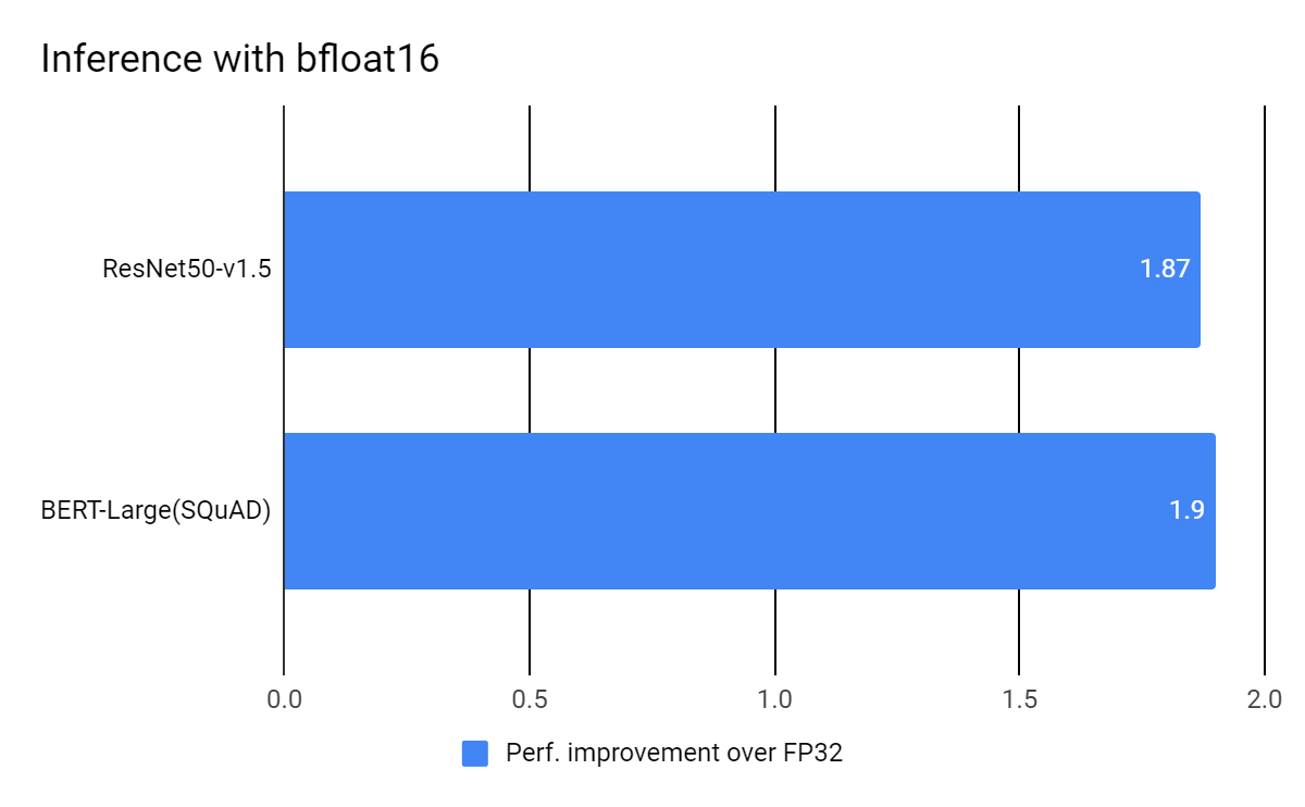
As shown in the charts above, training the models with mixed precision on a 3rd Gen Intel Xeon Scalable Processors with bfloat16 was 1.7x to 1.9x faster than FP32 precision on a 2nd Gen Intel Xeon Scalable Processors. Similarly, for inference, using bfloat16 precision resulted in a 1.87x to 1.9x performance increase.
Accuracy and time to train
In addition to performance measurements, we performed full convergence tests for the three deep learning models on two multi socket 3rd Gen Intel Xeon Scalable processor based systems*. For BERT-Large (SQuAD) and SSD-ResNet34, 4 socket 28 core systems were used. For ResNet50v1.5, we used an 8-socket 28 core system of 3rd Gen Intel Xeon Scalable processors. The models were first trained with FP32, and exactly the same hyper-parameters (learning rate etc.) and batch sizes were used to train the model with mixed precision.  The results above show that the models from three different use cases (image classification, language modeling, and object detection) are all able to reach SOTA accuracy using the same number of epochs. For ResNet50v1.5, the standard MLPerf threshold of 75.9% top-1 accuracy was used and both bfloat16 and FP32 reached the target accuracy in 84th epochs (evaluation every 4 epochs with eval offset of 0). For BERT-Large (SQuAD) fine-tuning task, both Bfloat16 and FP32 used two epochs. SSD-ResNet34, trained in 60 epochs. With the improved run time performance, the total time to train with bfloat16 was 1.7x to 1.9x better than the training time in FP32.
Intel-optimized Community build of TensorFlow
The Intel-optimized build of TensorFlow now supports Intel® Deep Learning Boost’s new bfloat16 capability for mixed precision training and low precision inference in the TensorFlow GitHub master branch. More information on the Intel build is available here. The models mentioned in this blog and scripts to run the models in bfloat16 and FP32 mode are available through the Model Zoo for Intel Architecture (v1.6.1 or later), which you can download and try from here. [Note: To run a bfloat16 model, you will need a Intel Xeon Scalable processor (Skylake) or later generation Intel Xeon Processor. However, to get the best performance of bfloat16 models, you will need a 3rd Gen Intel Xeon Scalable processor.]
Conclusion
As deep learning models get larger and more complicated, the combination of the latest 3rd Gen Intel Xeon Scalable processors with Intel Deep Learning Boost’s new bfloat16 format can achieve a performance increase of up to 1.7x to 1.9x over FP32 performance on 2nd Gen Intel® Xeon® Scalable Processors, without any loss of accuracy. We have enhanced the Intel -optimized build of TensorFlow so developers can easily port their models to use mixed precision training and inference with bfloat16. In addition, we have shown that the automatically-converted bfloat16 model does not need any additional tuning of hyperparameters to converge; you canuse the same set of hyperparameters that you used to train the FP32 models.
Acknowledgements
The results presented in this blog is the work of many people including the Intel TensorFlow and oneDNN teams and our collaborators in Google’s TensorFlow team.
From Intel – Jojimon Varghese , Xiaoming Cui, Md Faijul Amin, Niroop Ammbashankar, Mahmoud Abuzaina, Sharada Shiddibhavi, Chuanqi Wang, Yiqiang Li, Yang Sheng, Guizi Li, Teng Lu, Roma Dubstov, Tatyana Primak, Evarist Fomenko, Igor Safonov, Abhiram Krishnan, Shamima Najnin, Rajesh Poornachandran, Rajendrakumar Chinnaiyan.
From Google – Reed Wanderman-Milne, Penporn Koanantakool, Rasmus Larsen, Thiru Palaniswamy, Pankaj Kanwar.
*For configuration details see www.intel.com/3rd-gen-xeon-configs.
Notices and Disclaimers
Intel’s compilers may or may not optimize to the same degree for non-Intel microprocessors for optimizations that are not unique to Intel microprocessors. These optimizations include SSE2, SSE3, and SSSE3 instruction sets and other optimizations. Intel does not guarantee the availability, functionality, or effectiveness of any optimization on microprocessors not manufactured by Intel. Microprocessor-dependent optimizations in this product are intended for use with Intel microprocessors. Certain optimizations not specific to Intel microarchitecture are reserved for Intel microprocessors. Please refer to the applicable product User and Reference Guides for more information regarding the specific instruction sets covered by this notice.
Read More