Monthly Archives: October 2020

As the volume of unstructured data such as text and voice continues to grow, businesses are increasingly looking for ways to incorporate this data into their time series predictive modeling workflows. One example use case is transcribing calls from call centers to forecast call handle times and improve call volume forecasting. In the retail or media industry, companies are interested in using related information about products or content to forecast popularity of existing or new products or content from unstructured information such as product type, description, audience reviews, or social media feeds. However, combining this unstructured data with time series is challenging because most traditional time series models require numerical inputs for forecasting. In this post, we describe how you can combine Amazon SageMaker with Amazon Forecast to include unstructured text data into your time series use cases.

Solution overview

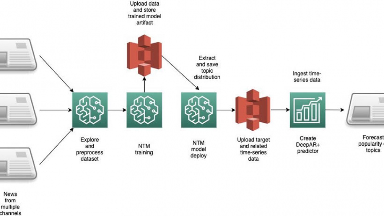
For our use case, we predict the popularity of news articles based on their topics looking forward over a 15 day horizon. You first download and preprocess the data and then run the NTM algorithm to generate topic vectors. After generating the topic vectors, you save them and use these vectors as a related time series to create the forecast.

The following diagram illustrates the architecture of this solution.

AWS services

Forecast is a fully managed service that uses machine learning (ML) to generate highly accurate forecasts without requiring any prior ML experience. Forecast is applicable in a wide variety of use cases, including energy demand forecasting, estimating product demand, workforce planning, and computing cloud infrastructure usage.

With Forecast, there are no servers to provision or ML models to build manually. Additionally, you only pay for what you use, and there is no minimum fee or upfront commitment. To use Forecast, you only need to provide historical data for what you want to forecast, and, optionally, any related data that you believe may impact your forecasts. This related data may include time-varying data (such as price, events, and weather) and categorical data (such as color, genre, or region). The service automatically trains and deploys ML models based on your data and provides you with a custom API to retrieve forecasts.

Amazon SageMaker is a fully managed service that provides every developer and data scientist with the ability to build, train, and deploy ML models quickly. The Neural Topic Model (NTM) algorithm is an unsupervised learning algorithm that can organize a collection of documents into topics that contain word groupings based on their statistical distribution. For example, documents that contain frequent occurrences of words such as “bike,” “car,” “train,” “mileage,” and “speed” are likely to share a topic on “transportation.” You can use topic modeling to classify or summarize documents based on the topics detected. You can also use it to retrieve information and recommend content based on topic similarities.

The derived topics that NTM learns are characterized as a latent representation because they are inferred from the observed word distributions in the collection. The semantics of topics are usually inferred by examining the top ranking words they contain. Because the method is unsupervised, only the number of topics, not the topics themselves, are pre-specified. In addition, the topics aren’t guaranteed to align with how a human might naturally categorize documents. NTM is one of the built-in algorithms you can train and deploy using Amazon SageMaker.

Prerequisites

To follow along with this post, you must create the following:

• An AWS Identity and Access Management (IAM role)
• An Amazon SageMaker notebook instance
• An Amazon Simple Storage Service (Amazon S3) bucket

To create the aforementioned resources and clone the forecast-samples GitHub repo into the notebook instance, launch the following AWS CloudFormation stack:

In the Parameters section, enter unique names for your S3 bucket and notebook and leave all other settings at their default.

When the CloudFormation script is complete, you can view the created resources on the Resources tab of the stack.

Navigate to Sagemaker and open the notebook instance created from the CloudFormation template. Open Jupyter and continue to the /notebooks/blog_materials/Time_Series_Forecasting_with_Unstructured_Data_and_Amazon_SageMaker_Neural_Topic_Model/ folder and start working your way through the notebooks.

Creating the resources manually

For the sake of completeness, we explain in detail the steps necessary to create the resources that the CloudFormation script creates automatically.

1. Create an IAM role that can do the following:
   1. Has permission to access Forecast and Amazon S3 to store the training and test datasets.
   2. Has an attached trust policy to give Amazon SageMaker permission to assume the role.
   3. Allows Forecast to access Amazon S3 to pull the stored datasets into Forecast.

For more information, see Set Up Permissions for Amazon Forecast.

2. Create an Amazon SageMaker notebook instance.
3. Attach the IAM role you created for Amazon SageMaker to this notebook instance.
4. Create an S3 bucket to store the outputs of your human workflow.
5. Copy the ARN of the bucket to use in the accompanying Jupyter notebook.

 This project consists of three notebooks, available in the GitHub repo. They cover the following:

• Preprocessing the dataset
• NTM with Amazon SageMaker
• Using Amazon Forecast to predict the topic’s popularity on various social media platforms going forward

Training and deploying the forecast

In the first notebook, 1_preprocess.ipynb, you download the New Popularity in Multiple Social Media Platforms dataset from the University of California Irvine (UCI) Machine Learning Repository using the requests library [1]. The following screenshot shows a sample of the dataset, where we have anonymized the topic names without loss of generality. It consists of news articles and their popularity on various social channels.

Because we’re focused on predictions based on the Headline and Title columns, we drop the Source and IDLink columns. We examine the current state of the data with a simple histogram plot. The following plot depicts the popularity of a subset of articles on Facebook.

The following plot depicts the popularity of a subset of articles on GooglePlus.

The distributions are heavily skewed towards a very small number of views; however, there are a few outlier articles that have an extremely high popularity.

Preprocessing the data

You may notice the popularity of the articles is extremely skewed. To convert this into a usable time series for ML, we need to convert the PublishDate column, which is read in as a string type, to a datetime type using the Pandas to_datetime method:

df['PublishDate'] = pd.to_datetime(df['PublishDate'], infer_datetime_format=True)

We then group by topic and save the preprocessed.csv to be used by the next notebook, 2_NTM.ipynb. In the directory /data, you should see a file called NewsRatingsdataset.csv. You can now move to the next notebook, where you build a neural topic model to extract topic vectors from the processed dataset.

Before creating the topic model, it’s helpful to explore the data some more. In the following code, we plot the daily time series for the popularity of a given topic across the three social media channels, as well as a daily time series for the sentiment of a topic based on news article titles and headlines:

topic = 1 # Change this to any of [0, 1, 2, 3]
subdf = df[(df['Topic']==topic)&(df['PublishDate']>START_DATE)]
subdf = subdf.reset_index().set_index('PublishDate')
subdf.index = pd.to_datetime(subdf.index)
subdf.head()
subdf[["LinkedIn", 'GooglePlus', 'Facebook']].resample("1D").mean().dropna().plot(figsize=(15, 4))
subdf[["SentimentTitle", 'SentimentHeadline']].resample("1D").mean().dropna().plot(figsize=(15, 4))

The following are the plots for the topic Topic_1.

The dataset still needs a bit more cleaning before it’s ready for the NTM algorithm to use. Not much data exists before October 13, 2015, so you can drop the data before that date and reset the indexes accordingly. Moreover, some of the headlines and ratings contain missing values, denoted by NaN and -1, respectively. You can use regex to find and replace those headlines with empty strings and convert these ratings to zeros. There is a difference in scale for the popularity of a topic on Facebook vs. LinkedIn vs. GooglePlus. For this post, you focus on forecasting popularity on Facebook only.

Topic modeling

Now you use the built-in NTM algorithm on Amazon SageMaker to extract topics from the news headlines. When preparing a corpus of documents for NTM, you must clean and standardize the data by converting the text to lower case, remove stop words, remove any numeric characters that may not be meaningful to your corpus, and tokenize the document’s text.

We use the Natural Language Toolkit and sklearn Python libraries to convert the headlines into tokens and create vectors of the token’s counts. Also, we drop the Title column in the dataframe, but store the titles in a separate dataframe. This is because the Headline column contains similar information as the Title column, but the headlines are longer and more descriptive, and we want to use the titles later on as a validation set for our NTM during training.

Lastly, we type cast the vectors into a sparse array in order to reduce the amount of memory utilization, because the bag-of-words matrix can quickly become quite large and memory intensive. For more information, see the notebook or Build a semantic content recommendation system with Amazon SageMaker.

Training an NTM

To extract text vectors, you convert each headline into a 20 (NUM_TOPICS)-dimensional topic vector. This can be viewed as an effective lower-dimensional embedding of all the text in the corpus into some predefined topics. Each topic has a representation as a vector, and related topics have a related vector representation. This topic is a derived topic and is not to be confused with the original Topic field in the raw dataset. Assuming that there is some correlation between topics from one day to the next (for example, the top topics don’t change very frequently on a daily basis), you can represent all the text in the dataset as a collection of 20 topics.

You then set the training dataset and trained model artifact location in Amazon S3 and upload the data. To train the model, you can use one or more instances (specified by the parameter train_instance_count) and choose a strategy to either fully replicate the data on each instance or use ShardedByS3Key, which only puts certain data shards on each instance. This speeds up training at the cost of each instance only seeing a fraction of the data.

To reduce overfitting, it’s helpful to introduce a validation dataset in addition to the training dataset. The hyperparameter num_patience_epochs controls the early stopping behavior, which makes sure the training is stopped if the change in the loss is less than the specified tolerance (set by tolerance) consistently for num_patience_epochs. The epochs hyperparameter specifies the total number of epochs to run the job. For this post, we chose hyperparameters to balance the tradeoff between accuracy and training time:

%time
from sagemaker.session import s3_input

sess = sagemaker.Session()
ntm = sagemaker.estimator.Estimator(container,
                                    role, 
                                    train_instance_count=1, 
                                    train_instance_type='ml.c4.xlarge',
                                    output_path=output_path,
                                    sagemaker_session=sess)
ntm.set_hyperparameters(num_topics=NUM_TOPICS, feature_dim=vocab_size, mini_batch_size=128, 
                        epochs=100, num_patience_epochs=5, tolerance=0.001)
s3_train = s3_input(s3_train_data, distribution='FullyReplicated') 
ntm.fit({'train': s3_train})

To further improve the model performance, you can take advantage of hyperparameter tuning in Amazon SageMaker.

Deploying and testing the model

To generate the feature vectors for the headlines, you first deploy the model and run inferences on the entire training dataset to obtain the topic vectors. An alternative option is to run a batch transform job.

To ensure that the topic model works as expected, we show the extracted topic vectors from the titles, and check if the topic distribution of the title is similar to that of the corresponding headline. Remember that the model hasn’t seen the titles before. As a measure of similarity, we compute the cosine similarity for a random title and associated headline. A high cosine similarity indicates that titles and headlines have a similar representation in this low-dimensional embedding space.

You can also use a cosine similarity of the title-headline as a feature: well-written titles that correlate well with the actual headline may obtain a higher popularity score. You could use this to check if titles and headlines represent the content of the document accurately, but we don’t explore this further in this notebook [2].

Finally, you store the results of the headlines mapped across the extracted NUM_TOPICS (20) back into a dataframe and save the dataframe as preprocessed_data.csv in data/ for use in subsequent notebooks.

The following code tests the vector similarity:

ntm_predictor = ntm.deploy(initial_instance_count=1, instance_type='ml.m4.xlarge')
topic_data = np.array(topic_vectors.tocsr()[:10].todense())
topic_vecs = []
for index in range(10):
    results = ntm_predictor.predict(topic_data[index])
    predictions = np.array([prediction['topic_weights'] for prediction in results['predictions']])
    topic_vecs.append(predictions)
from sklearn.metrics.pairwise import cosine_similarity
comparisonvec = []
for i, idx in enumerate(range(10)):
    comparisonvec.append([df.Headline[idx], title_column[idx], cosine_similarity(topic_vecs[i], [pred_array_cc[idx]])[0][0]])
pd.DataFrame(comparisonvec, columns=['Headline', 'Title', 'CosineSimilarity'])

The following screenshot shows the output.

Visualizing headlines

Another way to visualize the results is to plot a T-SNE graph. T-SNE uses a nonlinear embedding model by attempting to check if the nearest neighbor joint probability distribution in the high-dimensional space (for this use case, NUM_TOPICS) matches the equivalent lower-dimensional (2) joint distribution by minimizing a loss known as the Kullback-Leibler divergence [3]. Essentially, this is a dimensionality reduction technique that can map high-dimensional vectors to a lower-dimensional space.

Computing the T-SNE can take quite some time, especially for large datasets, so we shuffle the dataset and extract only 10,000 headline embeddings for the T-SNE plot. For more information about the advantages and pitfalls of using T-SNE in topic modeling, see How to Use t-SNE Effectively.

The following T-SNE plot shows a few large topics (indicated by the similar color clusters—red green, purple, blue, and brown), which is consistent with the dataset containing four primary topics. But by expanding the dimensionality of the topic vectors to NUM_TOPICS = 20, we allow the NTM model to capture additional semantic information between the headlines than is captured by a single topic token.

With our topic modeling complete and our data saved, you can now delete the endpoint to avoid incurring any charges.

Forecasting topic popularity

Now you run the third and final notebook, where you use the Forecast DeepAR+ algorithm to forecast the popularity of the topics. First, you establish a Forecast session using the Forecast SDK. It’s very important the region of your bucket is in the same region as the session.

After this step, you read in preprocessed_data.csv into a dataframe for some additional preprocessing. Drop the Headline column and replace the index of the dataframe with the publish date of the news article. You do this so you can easily aggregate the data on a daily basis. The following screenshot shows your results.

Creating the target and related time series

For this post, you want to forecast the Facebook ratings for each of the four topics in the Topic column of the dataset. In Forecast, we need to define a target time series that consists of the item ID, timestamp, and the value we want to forecast.

Additionally, as of this writing, you can provide a related time series, which can include up to 13 dynamic features, which in our use case are the SentimentHeadline and the topic vectors. Because we can only choose 13 features in Forecast, we choose 10 out of the 20 topic vectors to illustrate building the Forecast model. Currently, the CNN-QR, DeepAR+ algorithm (which we use in this post), and Prophet algorithm support related time series.

As before, we start forecasting from 2015-11-01 and end our training data at 2016-06-21. Using this, we forecast for 15 days into the future. The following screenshot shows our target time series.

The following screenshot shows our related time series.

Upload the datasets to the S3 bucket.

Defining the dataset schemas and dataset group to ingest into Forecast

Forecast has several predefined domains that come with predefined schemas for data ingestion. Because we’re interested in web traffic, you can choose the WEB_TRAFFIC domain. For more information about dataset domains, see Predefined Dataset Domains and Dataset Types.

This provides a predefined schema and attribute types for the attributes you include in the target and related time series. The WEB_TRAFFIC domain doesn’t have item metadata; only target and related time series data is allowed.

Define the schema for the target time series with the following code:

# Set the dataset name to a new unique value. If it already exists, go to the Forecast console and delete any existing
# dataset ARNs and datasets.

datasetName = 'webtraffic_forecast_NLP'

schema ={
   "Attributes":[
      {
         "AttributeName":"item_id",
         "AttributeType":"string"
      },    
       {
         "AttributeName":"timestamp",
         "AttributeType":"timestamp"
      },
      {
         "AttributeName":"value",
         "AttributeType":"float"
      }      
   ]
}

try:
    response = forecast.create_dataset(
                    Domain="WEB_TRAFFIC",
                    DatasetType='TARGET_TIME_SERIES',
                    DatasetName=datasetName,
                    DataFrequency=DATASET_FREQUENCY, 
                    Schema = schema
                   )
    datasetArn = response['DatasetArn']
    print('Success')
except Exception as e:
    print(e)
    datasetArn = 'arn:aws:forecast:{}:{}:dataset/{}'.format(REGION_NAME, ACCOUNT_NUM, datasetName)

Define the schema for the related time series with the following code:

# Set the dataset name to a new unique value. If it already exists, go to the Forecast console and delete any existing
# dataset ARNs and datasets.

datasetName = 'webtraffic_forecast_related_NLP'
schema ={
   "Attributes":[{
         "AttributeName":"item_id",
         "AttributeType":"string"
      }, 
       {
         "AttributeName":"timestamp",
         "AttributeType":"timestamp"
      },
       {
         "AttributeName":"SentimentHeadline",
         "AttributeType":"float"
      }]
    + 
      [{
         "AttributeName":"Headline_{}".format(x),
         "AttributeType":"float"
      } for x in range(10)] 
}

try:
    response=forecast.create_dataset(
                    Domain="WEB_TRAFFIC",
                    DatasetType='RELATED_TIME_SERIES',
                    DatasetName=datasetName,
                    DataFrequency=DATASET_FREQUENCY, 
                    Schema = schema
                   )
    related_datasetArn = response['DatasetArn']
    print('Success')
except Exception as e:
    print(e)
    related_datasetArn = 'arn:aws:forecast:{}:{}:dataset/{}'.format(REGION_NAME, ACCOUNT_NUM, datasetName)

Before ingesting any data into Forecast, we need to combine the target and related time series into a dataset group:

datasetGroupName = 'webtraffic_forecast_NLPgroup'
    
#try:
create_dataset_group_response = forecast.create_dataset_group(DatasetGroupName=datasetGroupName,
                                                              Domain="WEB_TRAFFIC",
                                                              DatasetArns= [datasetArn, related_datasetArn]
                                                             )
datasetGroupArn = create_dataset_group_response['DatasetGroupArn']
except Exception as e:
    datasetGroupArn = 'arn:aws:forecast:{}:{}:dataset-group/{}'.format(REGION_NAME, ACCOUNT_NUM, datasetGroupName)

Ingesting the target and related time series data from Amazon S3

Next you import the target and related data previously stored in AmazonS3 to create a Forecast dataset. You provide the location of the training data in Amazon S3 and the ARN of the dataset placeholder you created.

Ingest the target and related time series with the following code:

s3DataPath = 's3://{}/{}/target_time_series.csv'.format(bucket, prefix)
datasetImportJobName = 'forecast_DSIMPORT_JOB_TARGET'

try:
    ds_import_job_response=forecast.create_dataset_import_job(DatasetImportJobName=datasetImportJobName,
                                                          DatasetArn=datasetArn,
                                                          DataSource= {
                                                              "S3Config" : {
                                                                 "Path":s3DataPath,
                                                                 "RoleArn": role_arn
                                                              } 
                                                          },
                                                          TimestampFormat=TIMESTAMP_FORMAT
                                                         )
    ds_import_job_arn=ds_import_job_response['DatasetImportJobArn']
    target_ds_import_job_arn = copy.copy(ds_import_job_arn) #used to delete the resource during cleanup
except Exception as e:
    print(e)
    ds_import_job_arn='arn:aws:forecast:{}:{}:dataset-import-job/{}/{}'.format(REGION_NAME, ACCOUNT_NUM, datasetArn, datasetImportJobName)
s3DataPath = 's3://{}/{}/related_time_series.csv'.format(bucket, prefix)
datasetImportJobName = 'forecast_DSIMPORT_JOB_RELATED'
try:
    ds_import_job_response=forecast.create_dataset_import_job(DatasetImportJobName=datasetImportJobName,
                                                          DatasetArn=related_datasetArn,
                                                          DataSource= {
                                                              "S3Config" : {
                                                                 "Path":s3DataPath,
                                                                 "RoleArn": role_arn
                                                              } 
                                                          },
                                                          TimestampFormat=TIMESTAMP_FORMAT
                                                         )
    ds_import_job_arn=ds_import_job_response['DatasetImportJobArn']
    related_ds_import_job_arn = copy.copy(ds_import_job_arn) #used to delete the resource during cleanup
except Exception as e:
    print(e)
    ds_import_job_arn='arn:aws:forecast:{}:{}:dataset-import-job/{}/{}'.format(REGION_NAME, ACCOUNT_NUM, related_datasetArn, datasetImportJobName)

Creating the predictor

The Forecast DeepAR+ algorithm is a supervised learning algorithm for forecasting scalar (one-dimensional) time series using recurrent neural networks (RNNs). Classic forecasting methods, such as ARIMA or exponential smoothing (ETS), fit a single model to each individual time series. In contrast, DeepAR+ creates a global model (one model for all the time series) with the potential benefit of learning across time series.

The DeepAR+ model is particularly useful when working with a large collection (over thousands) of target time series, in which certain time series have a limited amount of information. For example, as a generalization of this use case, global models such as DeepAR+ can use the information from related topics with strong statistical signals to predict the popularity of new topics with little historical data. Importantly, DeepAR+ also allows you to include related information such as the topic vectors in a related time series.

To create the predictor, use the following code:

try:
    create_predictor_response=forecast.create_predictor(PredictorName=predictorName, 
                                                  ForecastHorizon=forecastHorizon,
                                                  AlgorithmArn=algorithmArn,
                                                  PerformAutoML=False, # change to true if want to perform AutoML
                                                  PerformHPO=False, # change to true to perform HPO
                                                  EvaluationParameters= {"NumberOfBacktestWindows": 1, 
                                                                         "BackTestWindowOffset": 15}, 
                                                  InputDataConfig= {"DatasetGroupArn": datasetGroupArn},
                                                  FeaturizationConfig= {"ForecastFrequency": "D", 
                                                                        }
                                                 )
    predictorArn=create_predictor_response['PredictorArn']
except Exception as e:
    predictorArn = 'arn:aws:forecast:{}:{}:predictor/{}'.format(REGION_NAME, ACCOUNT_NUM, predictorName)

When you call the create_predictor() method, it takes several minutes to complete.

Backtesting is a method of testing an ML model trained on and designed to predict time series data. Due to the sequential nature of time series data, training and test data can’t be randomized. Moreover, the most recent time series data is generally considered the most relevant for testing purposes. Therefore, backtesting uses the most recent windows that were unseen by the model during training to test the model and collect metrics. Amazon Forecast lets you choose up to five windows for backtesting. For more information, see Evaluating Predictor Accuracy.

For this post, we evaluate the DeepAR+ model for both the MAPE error, which is a common error metric in time series forecasting, and the root mean square error (RMSE), which penalizes larger deviations even more. The RMSE is an average deviation from the forecasted value and actual value in the same units as the dependent variable (in this use case, topic popularity on Facebook).

Creating and querying the forecast

When you’re satisfied with the accuracy metrics from your trained Forecast model, it’s time to generate a forecast. You can do this by creating a forecast for each item in the target time series used to train the predictor. Query the results to find out the popularity of the different topics in the original dataset.

The following is the result for Topic 0.

The following is the result for Topic 1.

The following is the result for Topic 2.

The following is the result for Topic 3.

Forecast accuracy

As an example, the RMSE for Topic 1 is 22.047559071991657. Although the actual range of popularity values in the ground truth set over the date range of the forecast is quite large [3:331], this RMSE does not in and of itself indicate if the model is production ready or not. The RMSE metric is simply an additional data point that should be used in the evaluation of the efficacy of your model.

Cleaning up

To avoid incurring future charges, delete each Forecast component. Also delete any other resources used in the notebook such as the Amazon SageMaker NTM endpoint, any S3 buckets used for storing data, and finally the Amazon SageMaker notebooks.

Conclusion

In this post, you learned how to build a forecasting model using unstructured raw text data. You also learned how to train a topic model and use the generated topic vectors as related time series for Forecast. Although this post is intended to demonstrate how you can combine these models together, you can improve the model accuracy by training on much larger datasets by having many more topics than in this dataset, using the same methodology.  Amazon Forecast also supports other deep learning models for time series forecasting such as CNN-Qr. To read more about how you can build an end-to-end operational workflow with Amazon Forecast and AWS StepFunctions, see here.

References

About the Authors

David Ehrlich is a Machine Learning Specialist at Amazon Web Services. He is passionate about helping customers unlock the true potential of their data. In his spare time, he enjoys exploring the different neighborhoods in New York City, going to comedy clubs, and traveling.

Stefan Natu is a Sr. Machine Learning Specialist at Amazon Web Services. He is focused on helping financial services customers build end-to-end machine learning solutions on AWS. In his spare time, he enjoys reading machine learning blogs, playing the guitar, and exploring the food scene in New York City.

Read More

Amazon Fraud Detector is a fully managed service that makes it easy to identify potentially fraudulent online activities, such as the creation of fake accounts or online payment fraud. Unlike general-purpose machine learning (ML) packages, Amazon Fraud Detector is designed specifically to detect fraud. Amazon Fraud Detector combines your data, the latest in ML science, and more than 20 years of fraud detection experience from Amazon.com and AWS to build ML models tailor-made to detect fraud in your business.

This post walks you through how to use Amazon Fraud Detector with Amazon Simple Storage Service (Amazon S3) and AWS Lambda to perform a batch of fraud predictions on event records (such as account registrations and transactions) in a CSV file. This architecture enables you to trigger a batch of predictions automatically upon uploading your CSV file to Amazon S3 and retrieve the fraud prediction results in a newly generated CSV also stored in Amazon S3.

Solution overview

Amazon Fraud Detector can perform low-latency fraud predictions, enabling your company to dynamically adjust the customer experience in your applications based on real-time fraud risk detection. But suppose you want to generate fraud predictions for a batch of events after the fact; perhaps you don’t need a low-latency response and want to evaluate events on an hourly or daily schedule. How do you accomplish this using Amazon Fraud Detector? One approach is to use an Amazon S3 event notification to trigger a Lambda function that processes a CSV file of events stored in Amazon S3 when the file is uploaded to an input S3 bucket. The function runs each event through Amazon Fraud Detector to generate predictions using a detector (ML model and rules) and uploads the prediction results to an S3 output bucket. The following diagram illustrates this architecture.

To create this Lambda-based batch prediction system, you complete the following high-level steps:

1. Create and publish a detector version containing a fraud detection model and rules, or simply a ruleset.
2. Create two S3 buckets. The first bucket is used to land your CSV file, and the second bucket is where your Lambda function writes the prediction results to.
3. Create an AWS Identity and Access Management (IAM) role to use as the execution role in the Lambda function.
4. Create a Lambda function that reads in a CSV file from Amazon S3, calls the Amazon Fraud Detector get_event_prediction function for each record in the CSV file, and writes a CSV file to Amazon S3.
5. Add an Amazon S3 event trigger to invoke your Lambda function whenever a new CSV file is uploaded to the S3 bucket.
6. Create a sample CSV file of event records to test the batch prediction process.
7. Test the end-to-end process by uploading your sample CSV file to your input S3 bucket and reviewing prediction results in the newly generated CSV file in your output S3 bucket.

Creating and publishing a detector

You can create and publish a detector version using the Amazon Fraud Detector console or via the APIs. For console instructions, see Get started (console) or Amazon Fraud Detector is now Generally Available. After you complete this step, note the following items, which you need in later steps:

• AWS Region you created the detector in
• Detector name and version
• Name of the entity type and event type used by your detector
• List of variables for the entity type used in your detector

The following screenshot shows the detail view of a detector version.

The following screenshot shows the detail view of an event type.

Creating the input and output S3 buckets

Create the following S3 buckets on the Amazon S3 console:

• fraud-detector-input – Where you upload the CSV file containing events for batch predictions
• fraud-detector-output – Where the Lambda function writes the prediction results file

Make sure you create your buckets in the same Region as your detector. For more information, see How do I create an S3 Bucket?

Creating the IAM role

To create the execution role in IAM that gives your Lambda function permission to access the AWS resources required for this solution, complete the following steps:

1. On the IAM console, choose Roles.
2. Choose Create role.
3. Select Lambda.
4. Choose Next.
5. Attach the following policies:
   • AWSLambdaBasicExecutionRole – Provides the Lambda function with write permissions to Amazon CloudWatch Logs.
   • AWSXRayDaemonWriteAccess – Allows the AWS X-Ray daemon to relay raw trace data and retrieve sampling data to be used by X-Ray.
   • AmazonFraudDetectorFullAccessPolicy – Provides permissions to create resources and generate fraud predictions in Amazon Fraud Detector.
   • AmazonS3FullAccess – Provides the Lambda function permissions to read and write objects in Amazon S3. This policy provides broad Amazon S3 access; as a best practice, consider reducing the scope of this policy to the S3 buckets required for this example, or use an inline policy such as the following:

{
    "Version": "2012-10-17",
    "Statement": [
        {
            "Sid": "VisualEditor0",
            "Effect": "Allow",
            "Action": [
                "s3:PutObject",
                "s3:GetObject"
            ],
            "Resource": [
                "arn:aws:s3:::fraud-detector-input/*",
                "arn:aws:s3:::fraud-detector-output/*"
            ]
        }
    ]
}

6. Choose Next.
7. Enter a name for your role (for example, lambda-s3-role).
8. Choose Create role.

Creating the Lambda function

Now let’s create our Lambda function on the Lambda console.

1. On the Lambda console, choose Create function.
2. For Function name, enter a name (for example, afd-batch-function).
3. For Runtime, choose Python 3.8.
4. For Execution role, select Use an existing role.
5. For Existing role, choose the role you created.

6. Choose Create function

Next, we walk through sections of the code used in the Lambda function. This code goes into the Function code section of your Lambda function. The full Lambda function code is available in the next section.

Packages

import json
import csv
import boto3

Defaults

# -- make a connection to fraud detector -- 
client = boto3.client("frauddetector")
# -- S3 bucket to write scored data to -- 
S3_BUCKET_OUT = "fraud-detector-output"
# -- specify event, entity, and detector  -- 
ENTITY_TYPE    = "customer"
EVENT_TYPE     = "new_account_registration_full_details"
DETECTOR_NAME  = "new_account_detector"
DETECTOR_VER   = "3"

We have entered the values from the detector we created and the output S3 bucket. Replace these default values with the values you used when creating your output S3 bucket and Amazon Fraud Detector resources.

Functions

We use a few helper functions along with the main lambda_handler() function:

• get_event_variables(EVENT_TYPE) – Returns a list of the variables for the event type. We map these to the input file positions.
• prep_record(record_map, event_map, line) – Returns a record containing just the data required by the detector.
• get_score(event, record) – Returns the fraud prediction risk scores and rule outcomes from the Amazon Fraud Detector get_event_predictionfunction. The get_score function uses two extra helper functions to format model scores (prep_scores) and rule outcomes (prep_outcomes).

Finally, the lambda_handler(event, context) drives the whole process. See the following example code:

get_event_variables(EVENT_TYPE)
def get_event_variables(EVENT_TYPE):
    """ return list of event variables 
    """
    response = client.get_event_types(name=EVENT_TYPE)
    event_variables = []

    for v in response['eventTypes'][0]['eventVariables']:
        event_variables.append(v)
    return event_variables
prep_record(record_map, event_map, line)
def prep_record(record_map, event_map, line):
    """ structure the record for scoring 
    """
    record = {}
    for key in record_map.keys():
        record[key] = line[record_map[key]]
        
    event = {}
    for key in event_map.keys():
        event[key] = line[event_map[key]]
    return record, event

prep_scores(model_scores)
def prep_scores(model_scores):
    """ return list of models and scores
    """
    detector_models = []
    for m in model_scores:
        detector_models.append(m['scores'])
    return detector_models

prep_outcomes(rule_results)
def prep_outcomes(rule_results):
    """ return list of rules and outcomes 
    """
    detector_outcomes = []
    for rule in rule_results:
        rule_outcomes ={}
        rule_outcomes[rule['ruleId']] = rule['outcomes']
        detector_outcomes.append(rule_outcomes)
    return detector_outcomes 

def get_score(event, record):
def get_score(event, record):
    """ return the score to the function
    """
    pred_rec = {}
    
    try:
        pred = client.get_event_prediction(detectorId=DETECTOR_NAME, 
                                       detectorVersionId=DETECTOR_VER,
                                       eventId = event['EVENT_ID'],
                                       eventTypeName = EVENT_TYPE,
                                       eventTimestamp = event['EVENT_TIMESTAMP'], 
                                       entities = [{'entityType': ENTITY_TYPE, 'entityId':event['ENTITY_ID']}],
                                       eventVariables=  record) 
                                       
        pred_rec["score"]   = prep_scores(pred['modelScores'])
        pred_rec["outcomes"]= prep_outcomes(pred['ruleResults'])

    except: 
        pred_rec["score"]   = [-999]
        pred_rec["outcomes"]= ["error"]
    
    return pred_rec

The following is the full code for the Lambda function:

import boto3 
import csv
import json

# -- make a connection to fraud detector -- 
client = boto3.client("frauddetector")

# -- S3 bucket to write batch predictions out to -- 
S3_BUCKET_OUT = "fraud-detector-output"

# -- specify event, entity, and detector  -- 
ENTITY_TYPE    = "customer"
EVENT_TYPE     = "new_account_registration_full_details"
DETECTOR_NAME  = "new_account_detector"
DETECTOR_VER   = "3"

def get_event_variables(EVENT_TYPE):
    """ return list of event variables 
    """
    response = client.get_event_types(name=EVENT_TYPE)
    event_variables = []

    for v in response['eventTypes'][0]['eventVariables']:
        event_variables.append(v)
    return event_variables

def prep_record(record_map, event_map, line):
    """ structure the record for scoring 
    """
    record = {}
    for key in record_map.keys():
        record[key] = line[record_map[key]]
        
    event = {}
    for key in event_map.keys():
        event[key] = line[event_map[key]]
    return record, event

def prep_scores(model_scores):
    """ return list of models and scores
    """
    detector_models = []
    for m in model_scores:
        detector_models.append(m['scores'])
    return detector_models

def prep_outcomes(rule_results):
    """return list of rules and outcomes
    """
    detector_outcomes = []
    for rule in rule_results:
        rule_outcomes = {}
        rule_outcomes[rule['ruleId']] = rule['outcomes']
        detector_outcomes.append(rule_outcomes)
    return detector_outcomes

def get_score(event, record):
    """ return the score to the function
    """
    pred_rec = {}
    
    try:
        pred = client.get_event_prediction(detectorId=DETECTOR_NAME, 
                                       detectorVersionId=DETECTOR_VER,
                                       eventId = event['EVENT_ID'],
                                       eventTypeName = EVENT_TYPE,
                                       eventTimestamp = event['EVENT_TIMESTAMP'], 
                                       entities = [{'entityType': ENTITY_TYPE, 'entityId':event['ENTITY_ID']}],
                                       eventVariables=  record) 
                                       
        pred_rec["score"]   = prep_scores(pred['modelScores'])
        pred_rec["outcomes"]= prep_outcomes(pred['ruleResults'])

    except: 
        pred_rec["score"]   = [-999]
        pred_rec["outcomes"]= ["error"]
    
    return pred_rec

def lambda_handler(event, context):
    """ the lambda event handler triggers the process. 
    """
    S3_BUCKET_IN = event['Records'][0]['s3']['bucket']['name']
    S3_FILE      = event['Records'][0]['s3']['object']['key']
    S3_OUT_FILE  = "batch_{0}".format(S3_FILE)
    
    
    # -- open a temp file to write predictions to. 
    f = open("/tmp/csv_file.csv", "w+")
    temp_csv_file = csv.writer(f) 
    
    # -- get the input file -- 
    s3    = boto3.resource('s3')
    obj   = s3.Object(S3_BUCKET_IN, S3_FILE)
    data  = obj.get()['Body'].read().decode('utf-8').splitlines()
    lines = csv.reader(data)
    
    # -- get the file header -- 
    file_variables = next(lines)
    
    # -- write the file header to temporary file -- 
    temp_csv_file.writerow(file_variables + ["MODEL_SCORES", "DETECTOR_OUTCOMES"])
    
    # -- get list of event variables -- 
    event_variables = get_event_variables(EVENT_TYPE)
    
    # -- map event variables to file structure -- 
    record_map = {}
    for var in event_variables:
        record_map[var] = file_variables.index(var)
    
    # -- map event fields to file structure --
    event_map = {}
    for var in ['ENTITY_ID', 'EVENT_ID', 'EVENT_TIMESTAMP']:
        event_map[var] = file_variables.index(var)
    
   # -- for each record in the file, prep it, score it, write it to temp. 
    for i,line in enumerate(lines):
        record, event       = prep_record(record_map, event_map, line)
        record_pred         = get_score(event, record)
        #print(list(record_pred.values()))
        temp_csv_file.writerow(line + list(record_pred.values()))
    
    
    # -- close the temp file and upload it to your OUTPUT bucket    
    f.close()
    s3_client = boto3.client('s3')
    s3_client.upload_file('/tmp/csv_file.csv', S3_BUCKET_OUT, "batch_pred_results_" + S3_FILE  )
    
    return {
        'statusCode': 200,
        'body': json.dumps('Batch Complete!')
    }

After you add the code to your Lambda function, choose Deploy to save.

Configuring your Lambda settings and creating the Amazon S3 trigger

The batch prediction processes require memory and time to process, so we need to change the Lambda function’s default memory allocation and maximum run time.

1. On the Lambda console, locate your function.
2. On the function detail page, under Basic settings, choose Edit.
3. For Memory, choose 2048 MB.
4. For Timeout, enter 15 min.
5. Choose Save.

A 15-minute timeout allows the function to process up to roughly 4,000 predictions per batch, so you should keep this in mind as you consider your CSV file creation and upload strategy.

You can now make it so that this Lambda function triggers when a CSV file is uploaded to your input S3 bucket.

6. At the top of the Lambda function detail page, in the Designer box, choose Add trigger.
7. Choose S3.
8. For Bucket, choose your input S3 bucket.
9. For Suffix, enter .csv.

A warning about recursive invocation appears. You don’t want to trigger a read and write to the same bucket, which is why you created a second S3 bucket for the output.

10. Select the check-box to acknowledge the recursive invocation warning.
11. Choose Add.

Creating a sample CSV file of event records

We need to create a sample CSV file of event records to test the batch prediction process. In this CSV file, include a column for each variable in your event type schema. In addition, include columns for:

• EVENT_ID – An identifier for the event, such as a transaction number. The field values must satisfy the following regular expression pattern: ^[0-9a-z_-]+$.
• ENTITY_ID – An identifier for the entity performing the event, such as an account number. The field values must also satisfy the following regular expression pattern: ^[0-9a-z_-]+$.
• EVENT_TIMESTAMP – A timestamp, in ISO 8601 format, for when the event occurred.

Column header names must match their corresponding Amazon Fraud Detector variable names exactly.

In your CSV file, each row corresponds to one event that you want to generate a prediction for. The following screenshot shows an example of a test CSV file.

For more information about Amazon Fraud Detector variable data types and formatting, see Create a variable.

Performing a test batch prediction

To test our Lambda function, we simply upload our test file to the fraud-detector-input S3 bucket via the Amazon S3 console. This triggers the Lambda function. We can then check the fraud-detector-output S3 bucket for the results file.

The following screenshot shows that the test CSV file 20_event_test.csv is uploaded to the fraud-detector-input S3 bucket.

When batch prediction is complete, the results CSV file batch_pred_results_20_event_test.csv is uploaded to the fraud-detector-output S3 bucket (see the following screenshot).

The following screenshots show our results CSV file. The new file has two new columns: MODEL_SCORES and DETECTOR_OUTCOMES. MODEL_SCORES contains model names, model details, and prediction scores for any models used in the detector. DETECTOR_OUTCOMES contains all rule results, including any matched rules and their corresponding outcomes.

If the results file doesn’t appear in the output S3 bucket, you can check the CloudWatch log stream to see if the Lambda function ran into any issues. To do this, go to your Lambda function on the Lambda console and choose the Monitoring tab, then choose View logs in CloudWatch. In CloudWatch, choose the log stream covering the time period you uploaded your CSV file.

Conclusion

Congrats! You have successfully performed a batch of fraud predictions. Depending on your use case, you may want to use your prediction results in other AWS services. For example, you can analyze the prediction results in Amazon QuickSight or send results that are high risk to Amazon Augmented AI (Amazon A2I) for a human review of the prediction.

Amazon Fraud Detector has a 2-month free trial that includes 30,000 predictions per month. After that, pricing starts at $0.005 per prediction for rules-only predictions and $0.03 for ML-based predictions. For more information, see Amazon Fraud Detector pricing. For more information about Amazon Fraud Detector, including links to additional blog posts, sample notebooks, user guide, and API documentation, see Amazon Fraud Detector.

The next step is to start dropping files into your S3 bucket! Good luck!

About the Authors

Nick Tostenrude is a Senior Manager of Product in AWS, where he leads the Amazon Fraud Detector service team. Nick joined Amazon nine years ago. He has spent the past four years as part of the AWS Fraud Prevention organization. Prior to AWS, Nick spent five years in Amazon’s Kindle and Devices organizations, leading product teams focused on the Kindle reading experience, accessibility, and K-12 Education.

Mike Ames is a Research Science Manager working on Amazon Fraud Detector. He helps companies use machine learning to combat fraud, waste and abuse. In his spare time, you can find him jamming to 90s metal with an electric mandolin.

Read More

References

[1] Multi-Source Social Feedback of Online News Feeds, N. Moniz and L. Torgo, arXiv:1801.07055 (2018).
[2] Learning to determine the quality of news headlines, Omidvar, A. et al. arXiv:1911.11139.
[3] “Visualizing data using T-SNE”, L., Van der Maaten and G. Hinton, Journal of Machine Learning Research 9 2579-2605 (2008).