PyTorch 1.7 released w/ CUDA 11, New APIs for FFTs, Windows support for Distributed training and more

Today, we’re announcing the availability of PyTorch 1.7, along with updated domain libraries. The PyTorch 1.7 release includes a number of new APIs including support for NumPy-Compatible FFT operations, profiling tools and major updates to both distributed data parallel (DDP) and remote procedure call (RPC) based distributed training. In addition, several features moved to stable including custom C++ Classes, the memory profiler, extensions via custom tensor-like objects, user async functions in RPC and a number of other features in torch.distributed such as Per-RPC timeout, DDP dynamic bucketing and RRef helper.

A few of the highlights include:

  • CUDA 11 is now officially supported with binaries available at PyTorch.org
  • Updates and additions to profiling and performance for RPC, TorchScript and Stack traces in the autograd profiler
  • (Beta) Support for NumPy compatible Fast Fourier transforms (FFT) via torch.fft
  • (Prototype) Support for Nvidia A100 generation GPUs and native TF32 format
  • (Prototype) Distributed training on Windows now supported
  • torchvision
    • (Stable) Transforms now support Tensor inputs, batch computation, GPU, and TorchScript
    • (Stable) Native image I/O for JPEG and PNG formats
    • (Beta) New Video Reader API
  • torchaudio
    • (Stable) Added support for speech rec (wav2letter), text to speech (WaveRNN) and source separation (ConvTasNet)

To reiterate, starting PyTorch 1.6, features are now classified as stable, beta and prototype. You can see the detailed announcement here. Note that the prototype features listed in this blog are available as part of this release.

Find the full release notes here.

Front End APIs

[Beta] NumPy Compatible torch.fft module

FFT-related functionality is commonly used in a variety of scientific fields like signal processing. While PyTorch has historically supported a few FFT-related functions, the 1.7 release adds a new torch.fft module that implements FFT-related functions with the same API as NumPy.

This new module must be imported to be used in the 1.7 release, since its name conflicts with the historic (and now deprecated) torch.fft function.

Example usage:

>>> import torch.fft
>>> t = torch.arange(4)
>>> t
tensor([0, 1, 2, 3])

>>> torch.fft.fft(t)
tensor([ 6.+0.j, -2.+2.j, -2.+0.j, -2.-2.j])

>>> t = tensor([0.+1.j, 2.+3.j, 4.+5.j, 6.+7.j])
>>> torch.fft.fft(t)
tensor([12.+16.j, -8.+0.j, -4.-4.j,  0.-8.j])

[Beta] C++ Support for Transformer NN Modules

Since PyTorch 1.5, we’ve continued to maintain parity between the python and C++ frontend APIs. This update allows developers to use the nn.transformer module abstraction from the C++ Frontend. And moreover, developers no longer need to save a module from python/JIT and load into C++ as it can now be used it in C++ directly.

[Beta] torch.set_deterministic

Reproducibility (bit-for-bit determinism) may help identify errors when debugging or testing a program. To facilitate reproducibility, PyTorch 1.7 adds the torch.set_deterministic(bool) function that can direct PyTorch operators to select deterministic algorithms when available, and to throw a runtime error if an operation may result in nondeterministic behavior. By default, the flag this function controls is false and there is no change in behavior, meaning PyTorch may implement its operations nondeterministically by default.

More precisely, when this flag is true:

  • Operations known to not have a deterministic implementation throw a runtime error;
  • Operations with deterministic variants use those variants (usually with a performance penalty versus the non-deterministic version); and
  • torch.backends.cudnn.deterministic = True is set.

Note that this is necessary, but not sufficient, for determinism within a single run of a PyTorch program. Other sources of randomness like random number generators, unknown operations, or asynchronous or distributed computation may still cause nondeterministic behavior.

See the documentation for torch.set_deterministic(bool) for the list of affected operations.

Performance & Profiling

[Beta] Stack traces added to profiler

Users can now see not only operator name/inputs in the profiler output table but also where the operator is in the code. The workflow requires very little change to take advantage of this capability. The user uses the autograd profiler as before but with optional new parameters: with_stack and group_by_stack_n. Caution: regular profiling runs should not use this feature as it adds significant overhead.

Distributed Training & RPC

[Stable] TorchElastic now bundled into PyTorch docker image

Torchelastic offers a strict superset of the current torch.distributed.launch CLI with the added features for fault-tolerance and elasticity. If the user is not be interested in fault-tolerance, they can get the exact functionality/behavior parity by setting max_restarts=0 with the added convenience of auto-assigned RANK and MASTER_ADDR|PORT (versus manually specified in torch.distributed.launch).

By bundling torchelastic in the same docker image as PyTorch, users can start experimenting with TorchElastic right-away without having to separately install torchelastic. In addition to convenience, this work is a nice-to-have when adding support for elastic parameters in the existing Kubeflow’s distributed PyTorch operators.

[Beta] Support for uneven dataset inputs in DDP

PyTorch 1.7 introduces a new context manager to be used in conjunction with models trained using torch.nn.parallel.DistributedDataParallel to enable training with uneven dataset size across different processes. This feature enables greater flexibility when using DDP and prevents the user from having to manually ensure dataset sizes are the same across different process. With this context manager, DDP will handle uneven dataset sizes automatically, which can prevent errors or hangs at the end of training.

[Beta] NCCL Reliability – Async Error/Timeout Handling

In the past, NCCL training runs would hang indefinitely due to stuck collectives, leading to a very unpleasant experience for users. This feature will abort stuck collectives and throw an exception/crash the process if a potential hang is detected. When used with something like torchelastic (which can recover the training process from the last checkpoint), users can have much greater reliability for distributed training. This feature is completely opt-in and sits behind an environment variable that needs to be explicitly set in order to enable this functionality (otherwise users will see the same behavior as before).

[Beta] TorchScript rpc_remote and rpc_sync

torch.distributed.rpc.rpc_async has been available in TorchScript in prior releases. For PyTorch 1.7, this functionality will be extended the remaining two core RPC APIs, torch.distributed.rpc.rpc_sync and torch.distributed.rpc.remote. This will complete the major RPC APIs targeted for support in TorchScript, it allows users to use the existing python RPC APIs within TorchScript (in a script function or script method, which releases the python Global Interpreter Lock) and could possibly improve application performance in multithreaded environment.

[Beta] Distributed optimizer with TorchScript support

PyTorch provides a broad set of optimizers for training algorithms, and these have been used repeatedly as part of the python API. However, users often want to use multithreaded training instead of multiprocess training as it provides better resource utilization and efficiency in the context of large scale distributed training (e.g. Distributed Model Parallel) or any RPC-based training application). Users couldn’t do this with with distributed optimizer before because we need to get rid of the python Global Interpreter Lock (GIL) limitation to achieve this.

In PyTorch 1.7, we are enabling the TorchScript support in distributed optimizer to remove the GIL, and make it possible to run optimizer in multithreaded applications. The new distributed optimizer has the exact same interface as before but it automatically converts optimizers within each worker into TorchScript to make each GIL free. This is done by leveraging a functional optimizer concept and allowing the distributed optimizer to convert the computational portion of the optimizer into TorchScript. This will help use cases like distributed model parallel training and improve performance using multithreading.

Currently, the only optimizer that supports automatic conversion with TorchScript is Adagrad and all other optimizers will still work as before without TorchScript support. We are working on expanding the coverage to all PyTorch optimizers and expect more to come in future releases. The usage to enable TorchScript support is automatic and exactly the same with existing python APIs, here is an example of how to use this:

import torch.distributed.autograd as dist_autograd
import torch.distributed.rpc as rpc
from torch import optim
from torch.distributed.optim import DistributedOptimizer

with dist_autograd.context() as context_id:
  # Forward pass.
  rref1 = rpc.remote("worker1", torch.add, args=(torch.ones(2), 3))
  rref2 = rpc.remote("worker1", torch.add, args=(torch.ones(2), 1))
  loss = rref1.to_here() + rref2.to_here()

  # Backward pass.
  dist_autograd.backward(context_id, [loss.sum()])

  # Optimizer, pass in optim.Adagrad, DistributedOptimizer will
  # automatically convert/compile it to TorchScript (GIL-free)
  dist_optim = DistributedOptimizer(
     optim.Adagrad,
     [rref1, rref2],
     lr=0.05,
  )
  dist_optim.step(context_id)

[Beta] Enhancements to RPC-based Profiling

Support for using the PyTorch profiler in conjunction with the RPC framework was first introduced in PyTorch 1.6. In PyTorch 1.7, the following enhancements have been made:

  • Implemented better support for profiling TorchScript functions over RPC
  • Achieved parity in terms of profiler features that work with RPC
  • Added support for asynchronous RPC functions on the server-side (functions decorated with rpc.functions.async_execution).

Users are now able to use familiar profiling tools such as with torch.autograd.profiler.profile() and with torch.autograd.profiler.record_function, and this works transparently with the RPC framework with full feature support, profiles asynchronous functions, and TorchScript functions.

[Prototype] Windows support for Distributed Training

PyTorch 1.7 brings prototype support for DistributedDataParallel and collective communications on the Windows platform. In this release, the support only covers Gloo-based ProcessGroup and FileStore.

To use this feature across multiple machines, please provide a file from a shared file system in init_process_group.

# initialize the process group
dist.init_process_group(
    "gloo",
    # multi-machine example:
    # init_method = "file://////{machine}/{share_folder}/file"
    init_method="file:///{your local file path}",
    rank=rank,
    world_size=world_size
)

model = DistributedDataParallel(local_model, device_ids=[rank])

Mobile

PyTorch Mobile supports both iOS and Android with binary packages available in Cocoapods and JCenter respectively. You can learn more about PyTorch Mobile here.

[Beta] PyTorch Mobile Caching allocator for performance improvements

On some mobile platforms, such as Pixel, we observed that memory is returned to the system more aggressively. This results in frequent page faults as PyTorch being a functional framework does not maintain state for the operators. Thus outputs are allocated dynamically on each execution of the op, for the most ops. To ameliorate performance penalties due to this, PyTorch 1.7 provides a simple caching allocator for CPU. The allocator caches allocations by tensor sizes and, is currently, available only via the PyTorch C++ API. The caching allocator itself is owned by client and thus the lifetime of the allocator is also maintained by client code. Such a client owned caching allocator can then be used with scoped guard, c10::WithCPUCachingAllocatorGuard, to enable the use of cached allocation within that scope.
Example usage:

#include <c10/mobile/CPUCachingAllocator.h>
.....
c10::CPUCachingAllocator caching_allocator;
  // Owned by client code. Can be a member of some client class so as to tie the
  // the lifetime of caching allocator to that of the class.
.....
{
  c10::optional<c10::WithCPUCachingAllocatorGuard> caching_allocator_guard;
  if (FLAGS_use_caching_allocator) {
    caching_allocator_guard.emplace(&caching_allocator);
  }
  ....
  model.forward(..);
}
...

NOTE: Caching allocator is only available on mobile builds, thus the use of caching allocator outside of mobile builds won’t be effective.

torchvision

[Stable] Transforms now support Tensor inputs, batch computation, GPU, and TorchScript

torchvision transforms are now inherited from nn.Module and can be torchscripted and applied on torch Tensor inputs as well as on PIL images. They also support Tensors with batch dimensions and work seamlessly on CPU/GPU devices:

import torch
import torchvision.transforms as T

# to fix random seed, use torch.manual_seed
# instead of random.seed
torch.manual_seed(12)

transforms = torch.nn.Sequential(
    T.RandomCrop(224),
    T.RandomHorizontalFlip(p=0.3),
    T.ConvertImageDtype(torch.float),
    T.Normalize([0.485, 0.456, 0.406], [0.229, 0.224, 0.225])
)
scripted_transforms = torch.jit.script(transforms)
# Note: we can similarly use T.Compose to define transforms
# transforms = T.Compose([...]) and 
# scripted_transforms = torch.jit.script(torch.nn.Sequential(*transforms.transforms))

tensor_image = torch.randint(0, 256, size=(3, 256, 256), dtype=torch.uint8)
# works directly on Tensors
out_image1 = transforms(tensor_image)
# on the GPU
out_image1_cuda = transforms(tensor_image.cuda())
# with batches
batched_image = torch.randint(0, 256, size=(4, 3, 256, 256), dtype=torch.uint8)
out_image_batched = transforms(batched_image)
# and has torchscript support
out_image2 = scripted_transforms(tensor_image)

These improvements enable the following new features:

  • support for GPU acceleration
  • batched transformations e.g. as needed for videos
  • transform multi-band torch tensor images (with more than 3-4 channels)
  • torchscript transforms together with your model for deployment
    Note: Exceptions for TorchScript support includes Compose, RandomChoice, RandomOrder, Lambda and those applied on PIL images, such as ToPILImage.

[Stable] Native image IO for JPEG and PNG formats

torchvision 0.8.0 introduces native image reading and writing operations for JPEG and PNG formats. Those operators support TorchScript and return CxHxW tensors in uint8 format, and can thus be now part of your model for deployment in C++ environments.

from torchvision.io import read_image

# tensor_image is a CxHxW uint8 Tensor
tensor_image = read_image('path_to_image.jpeg')

# or equivalently
from torchvision.io import read_file, decode_image
# raw_data is a 1d uint8 Tensor with the raw bytes
raw_data = read_file('path_to_image.jpeg')
tensor_image = decode_image(raw_data)

# all operators are torchscriptable and can be
# serialized together with your model torchscript code
scripted_read_image = torch.jit.script(read_image)

[Stable] RetinaNet detection model

This release adds pretrained models for RetinaNet with a ResNet50 backbone from Focal Loss for Dense Object Detection.

[Beta] New Video Reader API

This release introduces a new video reading abstraction, which gives more fine-grained control of iteration over videos. It supports image and audio, and implements an iterator interface so that it is interoperable with other the python libraries such as itertools.

from torchvision.io import VideoReader

# stream indicates if reading from audio or video
reader = VideoReader('path_to_video.mp4', stream='video')
# can change the stream after construction
# via reader.set_current_stream

# to read all frames in a video starting at 2 seconds
for frame in reader.seek(2):
    # frame is a dict with "data" and "pts" metadata
    print(frame["data"], frame["pts"])

# because reader is an iterator you can combine it with
# itertools
from itertools import takewhile, islice
# read 10 frames starting from 2 seconds
for frame in islice(reader.seek(2), 10):
    pass
    
# or to return all frames between 2 and 5 seconds
for frame in takewhile(lambda x: x["pts"] < 5, reader):
    pass

Notes:

  • In order to use the Video Reader API beta, you must compile torchvision from source and have ffmpeg installed in your system.
  • The VideoReader API is currently released as beta and its API may change following user feedback.

torchaudio

With this release, torchaudio is expanding its support for models and end-to-end applications, adding a wav2letter training pipeline and end-to-end text-to-speech and source separation pipelines. Please file an issue on github to provide feedback on them.

[Stable] Speech Recognition

Building on the addition of the wav2letter model for speech recognition in the last release, we’ve now added an example wav2letter training pipeline with the LibriSpeech dataset.

[Stable] Text-to-speech

With the goal of supporting text-to-speech applications, we added a vocoder based on the WaveRNN model, based on the implementation from this repository. The original implementation was introduced in “Efficient Neural Audio Synthesis”. We also provide an example WaveRNN training pipeline that uses the LibriTTS dataset added to torchaudio in this release.

[Stable] Source Separation

With the addition of the ConvTasNet model, based on the paper “Conv-TasNet: Surpassing Ideal Time-Frequency Magnitude Masking for Speech Separation,” torchaudio now also supports source separation. An example ConvTasNet training pipeline is provided with the wsj-mix dataset.

Cheers!

Team PyTorch

Read More

Bringing real-time machine learning-powered insights to rugby using Amazon SageMaker

Bringing real-time machine learning-powered insights to rugby using Amazon SageMaker

The Guinness Six Nations Championship began in 1883 as the Home Nations Championship among England, Ireland, Scotland, and Wales, with the inclusion of France in 1910 and Italy in 2000. It is among the oldest surviving rugby traditions and one of the best-attended sporting events in the world. The COVID-19 outbreak disrupted the end of the 2020 Championship and four games were postponed. The remaining rounds resumed on October 24. With the increasing application of artificial intelligence and machine learning (ML) in sports analytics, AWS and Stats Perform partnered to bring ML-powered, real-time stats to the game of rugby, to enhance fan engagement and provide valuable insights into the game.

This post summarizes the collaborative effort between the Guinness Six Nations Rugby Championship, Stats Perform, and AWS to develop an ML-driven approach with Amazon SageMaker and other AWS services that predicts the probability of a successful penalty kick, computed in real time and broadcast live during the game. AWS infrastructure enables single-digit millisecond latency for kick predictions during inference. The Kick Predictor stat is one of the many new AWS-powered, on-screen dynamic Matchstats that provide fans with a greater understanding of key in-game events, including scrum analysis, play patterns, rucks and tackles, and power game analysis. For more information about other stats developed for rugby using AWS services, see the Six Nations Rugby website.

Rugby is a form of football with a 23-player match day squad. 15 players on each team are on the field, with additional substitutions waiting to get involved in the full-contact sport. The objective of the game is to outscore the opposing team, and one way of scoring is to kick a goal. The ability to kick accurately is one of the most critical elements of rugby, and there are two ways to score with a kick: through a conversion (worth two points) and a penalty (worth three points).

Predicting the likelihood of a successful kick is important because it enhances fan engagement during the game by showing the success probability before the player kicks the ball. There are usually 40–60 seconds of stoppage time while the player sets up for the kick, during which the Kick Predictor stat can appear on-screen to fans. Commentators also have time to predict the outcome, quantify the difficulty of each kick, and compare kickers in similar situations. Moreover, teams may start to use kicking probability models in the future to determine which player should kick given the position of the penalty on the pitch.

Developing an ML solution

To calculate the penalty success probability, the Amazon Machine Learning Solutions Lab used Amazon SageMaker to train, test, and deploy an ML model from historical in-game events data, which calculates the kick predictions from anywhere in the field. The following sections explain the dataset and preprocessing steps, the model training, and model deployment procedures.

Dataset and preprocessing

Stats Perform provided the dataset for training the goal kick model. It contained millions of events from historical rugby matches from 46 leagues from 2007–2019. The raw JSON events data that was collected during live rugby matches was ingested and stored on Amazon Simple Storage Service (Amazon S3). It was then parsed and preprocessed in an Amazon SageMaker notebook instance. After selecting the kick-related events, the training data comprised approximately 67,000 kicks, with approximately 50,000 (75%) successful kicks and 17,000 misses (25%).

The following graph shows a summary of kicks taken during a sample game. The athletes kicked from different angles and various distances.

Rugby experts contributed valuable insights to the data preprocessing, which included detecting and removing anomalies, such as unreasonable kicks. The clean CSV data went back to an S3 bucket for ML training.

The following graph depicts the heatmap of the kicks after preprocessing. The left-side kicks are mirrored. The brighter colors indicated a higher chance of scoring, standardized between 0 to 1.

Feature engineering

To better capture the real-world event, the ML Solutions Lab engineered several features using exploratory data analysis and insights from rugby experts. The features that went into the modeling fell into three main categories:

  • Location-based features – The zone in which the athlete takes the kick and the distance and angle of the kick to the goal. The x-coordinates of the kicks are mirrored along the center of the rugby pitch to eliminate the left or right bias in the model.
  • Player performance features – The mean success rates of the kicker in a given field zone, in the Championship, and in the kicker’s entire career.
  • In-game situational features – The kicker’s team (home or away), the scoring situation before they take the kick, and the period of the game in which they take the kick.

The location-based and player performance features are the most important features in the model.

After feature engineering, the categorical variables were one-hot encoded, and to avoid the bias of the model towards large-value variables, the numerical predictors were standardized. During the model training phase, a player’s historical performance features were pushed to Amazon DynamoDB tables. DynamoDB helped provide single-digit millisecond latency for kick predictions during inference.

Training and deploying models

To explore a wide range of classification algorithms (such as logistic regression, random forests, XGBoost, and neural networks), a 10-fold stratified cross-validation approach was used for model training. After exploring different algorithms, the built-in XGBoost in Amazon SageMaker was used due to its better prediction performance and inference speed. Additionally, its implementation has a smaller memory footprint, better logging, and improved hyperparameter optimization (HPO) compared to the original code base.

HPO, or tuning, is the process of choosing a set of optimal hyperparameters for a learning algorithm, and is a challenging element in any ML problem. HPO in Amazon SageMaker uses an implementation of Bayesian optimization to choose the best hyperparameters for the next training job. Amazon SageMaker HPO automatically launches multiple training jobs with different hyperparameter settings, evaluates the results of those training jobs based on a predefined objective metric, and selects improved hyperparameter settings for future attempts based on previous results.

The following diagram illustrates the model training workflow.

Optimizing hyperparameters in Amazon SageMaker

You can configure training jobs and when the hyperparameter tuning job launches by initializing an estimator, which includes the container image for the algorithm (for this use case, XGBoost), configuration for the output of the training jobs, the values of static algorithm hyperparameters, and the type and number of instances to use for the training jobs. For more information, see Train a Model.

To create the XGBoost estimator for this use case, enter the following code:

import boto3
import sagemaker
from sagemaker.tuner import IntegerParameter, CategoricalParameter, ContinuousParameter, HyperparameterTuner
from sagemaker.amazon.amazon_estimator import get_image_uri
BUCKET = <bucket name>
PREFIX = 'kicker/xgboost/'
region = boto3.Session().region_name
role = sagemaker.get_execution_role()
smclient = boto3.Session().client('sagemaker')
sess = sagemaker.Session()
s3_output_path = ‘s3://{}/{}/output’.format(BUCKET, PREFIX)

container = get_image_uri(region, 'xgboost', repo_version='0.90-1')

xgb = sagemaker.estimator.Estimator(container,
                                    role, 
                                    train_instance_count=4, 
                                    train_instance_type= 'ml.m4.xlarge',
                                    output_path=s3_output_path,
                                    sagemaker_session=sess)

After you create the XGBoost estimator object, set its initial hyperparameter values as shown in the following code:

xgb.set_hyperparameters(eval_metric='auc',
                        objective= 'binary:logistic',
			num_round=200,
                        rate_drop=0.3,
                        max_depth=5,
                        subsample=0.8,
                        gamma=2,
                        eta=0.2,
                        scale_pos_weight=2.85) #For class imbalance weights

# Specifying the objective metric (auc on validation set)
OBJECTIVE_METRIC_NAME = ‘validation:auc’

# specifying the hyper parameters and their ranges
HYPERPARAMETER_RANGES = {'eta': ContinuousParameter(0, 1),
                        'alpha': ContinuousParameter(0, 2),
                        'max_depth': IntegerParameter(1, 10)}

For this post, AUC (area under the ROC curve) is the evaluation metric. This enables the tuning job to measure the performance of the different training jobs. The kick prediction is also a binary classification problem, which is specified in the objective argument as a binary:logistic. There is also a set of XGBoost-specific hyperparameters that you can tune. For more information, see Tune an XGBoost model.

Next, create a HyperparameterTuner object by indicating the XGBoost estimator, the hyperparameter ranges, passing the parameters, the objective metric name and definition, and tuning resource configurations, such as the number of training jobs to run in total and how many training jobs can run in parallel. Amazon SageMaker extracts the metric from Amazon CloudWatch Logs with a regular expression. See the following code:

tuner = HyperparameterTuner(xgb,
                            OBJECTIVE_METRIC_NAME,
                            HYPERPARAMETER_RANGES,
                            max_jobs=20,
                            max_parallel_jobs=4)
s3_input_train = sagemaker.s3_input(s3_data='s3://{}/{}/train'.format(BUCKET, PREFIX), content_type='csv')
s3_input_validation = sagemaker.s3_input(s3_data='s3://{}/{}/validation/'.format(BUCKET, PREFIX), content_type='csv')
tuner.fit({'train': s3_input_train, 'validation':

Finally, launch a hyperparameter tuning job by calling the fit() function. This function takes the paths of the training and validation datasets in the S3 bucket. After you create the hyperparameter tuning job, you can track its progress via the Amazon SageMaker console. The training time depends on the instance type and number of instances you selected during tuning setup.

Deploying the model on Amazon SageMaker

When the training jobs are complete, you can deploy the best performing model. If you’d like to compare models for A/B testing, Amazon SageMaker supports hosting representational state transfer (REST) endpoints for multiple models. To set this up, create an endpoint configuration that describes the distribution of traffic across the models. In addition, the endpoint configuration describes the instance type required for model deployment. The first step is to get the name of the best performing training job and create the model name.

After you create the endpoint configuration, you’re ready to deploy the actual endpoint for serving inference requests. The result is an endpoint that can you can validate and incorporate into production applications. For more information about deploying models, see Deploy the Model to Amazon SageMaker Hosting Services. To create the endpoint configuration and deploy it, enter the following code:

endpoint_name = 'Kicker-XGBoostEndpoint'
xgb_predictor = tuner.deploy(initial_instance_count=1, 
                             instance_type='ml.t2.medium', 
                             endpoint_name=endpoint_name)

After you create the endpoint, you can request a prediction in real time.

Building a RESTful API for real-time model inference

You can create a secure and scalable RESTful API that enables you to request the model prediction based on the input values. It’s easy and convenient to develop different APIs using AWS services.

The following diagram illustrates the model inference workflow.

First, you request the probability of the kick conversion by passing parameters through Amazon API Gateway, such as the location and zone of the kick, kicker ID, league and Championship ID, the game’s period, if the kicker’s team is playing home or away, and the team score status.

The API Gateway passes the values to the AWS Lambda function, which parses the values and requests additional features related to the player’s performance from DynamoDB lookup tables. These include the mean success rates of the kicking player in a given field zone, in the Championship, and in the kicker’s entire career. If the player doesn’t exist in the database, the model uses the average performance in the database in the given kicking location. After the function combines all the values, it standardizes the data and sends it to the Amazon SageMaker model endpoint for prediction.

The model performs the prediction and returns the predicted probability to the Lambda function. The function parses the returned value and sends it back to API Gateway. API Gateway responds with the output prediction. The end-to-end process latency is less than a second.

The following screenshot shows example input and output of the API. The RESTful API also outputs the average success rate of all the players in the given location and zone to get the comparison of the player’s performance with the overall average.

For instructions on creating a RESTful API, see Call an Amazon SageMaker model endpoint using Amazon API Gateway and AWS Lambda.

Bringing design principles into sports analytics

To create the first real-time prediction model for the tournament with a millisecond latency requirement, the ML Solutions Lab team worked backwards to identify areas in which design thinking could save time and resources. The team worked on an end-to-end notebook within an Amazon SageMaker environment, which enabled data access, raw data parsing, data preprocessing and visualization, feature engineering, model training and evaluation, and model deployment in one place. This helped in automating the modeling process.

Moreover, the ML Solutions Lab team implemented a model update iteration for when the model was updated with newly generated data, in which the model parses and processes only the additional data. This brings computational and time efficiencies to the modeling.

In terms of next steps, the Stats Perform AI team has been looking at the next stage of rugby analysis by breaking down the other strategic facets as line-outs, scrums and teams, and continuous phases of play using the fine-grain spatio-temporal data captured. The state-of-the-art feature representations and latent factor modelling (which have been utilized so effectively in Stats Perform’s “Edge” match-analysis and recruitment products in soccer) means that there is plenty of fertile space for innovation that can be explored in rugby.

Conclusion

Six Nations Rugby, Stats Perform, and AWS came together to bring the first real-time prediction model to the 2020 Guinness Six Nations Rugby Championship. The model determined a penalty or conversion kick success probability from anywhere in the field. They used Amazon SageMaker to build, train, and deploy the ML model with variables grouped into three main categories: location-based features, player performance features, and in-game situational features. The Amazon SageMaker endpoint provided prediction results with subsecond latency. The model was used by broadcasters during the live games in the Six Nations 2020 Championship, bringing a new metric to millions of rugby fans.

You can find full, end-to-end examples of creating custom training jobs, training state-of-the-art object detection models, and model deployment on Amazon SageMaker on the AWS Labs GitHub repo. To learn more about the ML Solutions Lab, see Amazon Machine Learning Solutions Lab.


About the Authors

Mehdi Noori is a Data Scientist at the Amazon ML Solutions Lab, where he works with customers across various verticals, and helps them to accelerate their cloud migration journey, and to solve their ML problems using state-of-the-art solutions and technologies.


Tesfagabir Meharizghi is a Data Scientist at the Amazon ML Solutions Lab where he works with customers across different verticals accelerate their use of artificial intelligence and AWS cloud services to solve their business challenges. Outside of work, he enjoys spending time with his family and reading books.


Patrick Lucey is the Chief Scientist at Stats Perform. Patrick started the Artificial Intelligence group at Stats Perform in 2015, with thegroup focusing on both computer vision and predictive modelling capabilities in sport. Previously, he was at Disney Research for 5 years, where he conducted research into automatic sports broadcasting using large amounts of spatiotemporal tracking data. He received his BEng(EE) from USQ and PhD from QUT, Australia in 2003 and 2008 respectively. He was also co-author of the best paper at the 2016 MIT Sloan Sports Analytics Conference and in 2017 & 2018 was co-author of best-paper runner-up at the same conference.


Xavier Ragot is Data Scientist with the Amazon ML Solution Lab team where he helps design creative ML solution to address customers’ business problems in various industries.
Read More

Building an NLU-powered search application with Amazon SageMaker and the Amazon ES KNN feature

Building an NLU-powered search application with Amazon SageMaker and the Amazon ES KNN feature

The rise of semantic search engines has made ecommerce and retail businesses search easier for its consumers. Search engines powered by natural language understanding (NLU) allow you to speak or type into a device using your preferred conversational language rather than finding the right keywords for fetching the best results. You can query using words or sentences in your native language, leaving it to the search engine to deliver the best results.

Amazon SageMaker is a fully managed service that provides every developer and data scientist with the ability to build, train, and deploy machine learning (ML) models quickly. Amazon Elasticsearch Service (Amazon ES) is a fully managed service that makes it easy for you to deploy, secure, and run Elasticsearch cost-effectively at scale. Amazon ES offers KNN search, which can enhance search in use cases such as product recommendations, fraud detection, and image, video, and some specific semantic scenarios like document and query similarity. Alternatively, you can also choose Amazon Kendra, a highly accurate and easy to use enterprise search service that’s powered by machine learning, with no machine learning experience required. In this post, we explain how you can implement an NLU-based product search for certain types of applications using Amazon SageMaker and the Amazon ES k-nearest neighbor (KNN) feature.

In the post Building a visual search application with Amazon SageMaker and Amazon ES, we shared how to build a visual search application using Amazon SageMaker and the Amazon ES KNN’s Euclidean distance metric. Amazon ES now supports open-source Elasticsearch version 7.7 and includes the cosine similarity metric for KNN indexes. Cosine similarity measures the cosine of the angle between two vectors in the same direction, where a smaller cosine angle denotes higher similarity between the vectors. With cosine similarity, you can measure the orientation between two vectors, which makes it the ideal choice for some specific semantic search applications. The highly distributed architecture of Amazon ES enables you to implement an enterprise-grade search engine with enhanced KNN ranking, with high recall and performance.

In this post, you build a very simple search application that demonstrates the potential of using KNN with Amazon ES compared to the traditional Amazon ES ranking method, including a web application for testing the KNN-based search queries in your browser. The application also compares the search results with Elasticsearch match queries to demonstrate the difference between KNN search and full-text search.

Overview of solution

Regular Elasticsearch text-matching search is useful when you want to do text-based search, but KNN-based search is a more natural way to search for something. For example, when you search for a wedding dress using KNN-based search application, it gives you similar results if you type “wedding dress” or “marriage dress.” Implementing this KNN-based search application consists of two phases:

  • KNN reference index – In this phase, you pass a set of corpus documents through a deep learning model to extract their features, or embeddings. Text embeddings are a numerical representation of the corpus. You save those features into a KNN index on Amazon ES. The concept underpinning KNN is that similar data points exist in close proximity in the vector space. As an example, “summer dress” and “summer flowery dress” are both similar, so these text embeddings are collocated, as opposed to “summer dress” vs. “wedding dress.”
  • KNN index query – This is the inference phase of the application. In this phase, you submit a text search query through the deep learning model to extract the features. Then, you use those embeddings to query the reference KNN index. The KNN index returns similar text embeddings from the KNN vector space. For example, if you pass a feature vector of “marriage dress” text, it returns “wedding dress” embeddings as a similar item.

Next, let’s take a closer look at each phase in detail, with the associated AWS architecture.

KNN reference index creation

For this use case, you use dress images and their visual descriptions from the Feidegger dataset. This dataset is a multi-modal corpus that focuses specifically on the domain of fashion items and their visual descriptions in German. The dataset was created as part of ongoing research at Zalando into text-image multi-modality in the area of fashion.

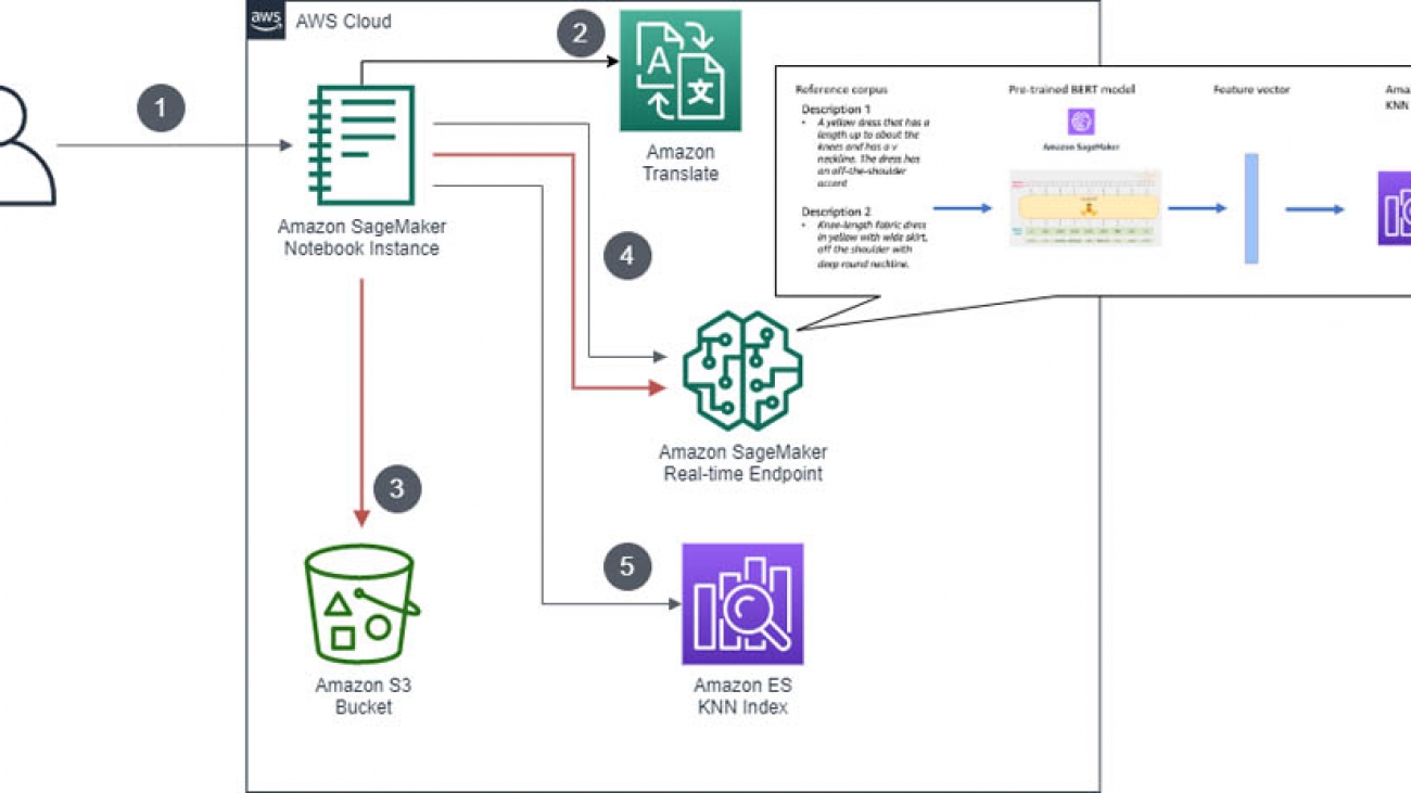
In this step, you translate each dress description from German to English using Amazon Translate. From each English description, you extract the feature vector, which is an n-dimensional vector of numerical features that represent the dress. You use a pre-trained BERT model hosted in Amazon SageMaker to extract 768 feature vectors of each visual description of the dress, and store them as a KNN index in an Amazon ES domain.

The following screenshot illustrates the workflow for creating the KNN index.

The process includes the following steps:

  1. Users interact with a Jupyter notebook on an Amazon SageMaker notebook instance. An Amazon SageMaker notebook instance is an ML compute instance running the Jupyter Notebook app. Amazon SageMaker manages creating the instance and related resources.
  2. Each item description, originally open-sourced in German, is translated to English using Amazon Translate.
  3. A pre-trained BERT model is downloaded, and the model artifact is serialized and stored in Amazon Simple Storage Service (Amazon S3). The model is used to serve from a PyTorch model server on an Amazon SageMaker real-time endpoint.
  4. Translated descriptions are pushed through the SageMaker endpoint to extract fixed-length features (embeddings).
  5. The notebook code writes the text embeddings to the KNN index along with product Amazon S3 URI in an Amazon ES domain.

KNN search from a query text

In this step, you present a search query text string from the application, which passes through the Amazon SageMaker hosted model to extract 768 features. You use these features to query the KNN index in Amazon ES. KNN for Amazon ES lets you search for points in a vector space and find the nearest neighbors for those points by cosine similarity (the default is Euclidean distance). When it finds the nearest neighbors vectors (for example, k = 3 nearest neighbors) for a given query text, it returns the associated Amazon S3 images to the application. The following diagram illustrates the KNN search full-stack application architecture.

The process includes the following steps:

  1. The end-user accesses the web application from their browser or mobile device.
  2. A user-provided search query string is sent to Amazon API Gateway and AWS Lambda.
  3. The Lambda function invokes the Amazon SageMaker real-time endpoint, and the model returns a vector of the search query embeddings. Amazon SageMaker hosting provides a managed HTTPS endpoint for predictions and automatically scales to the performance needed for your application using Application Auto Scaling.
  4. The function passes the search query embedding vector as the search value for a KNN search in the index in the Amazon ES domain. A list of k similar items and their respective Amazon S3 URIs are returned.
  5. The function generates pre-signed Amazon S3 URLs to return back to the client web application, used to display similar items in the browser.

Prerequisites

For this walkthrough, you should have an AWS account with appropriate AWS Identity and Access Management (IAM) permissions to launch the AWS CloudFormation template.

Deploying your solution

You use a CloudFormation stack to deploy the solution. The stack creates all the necessary resources, including the following:

  • An Amazon SageMaker notebook instance to run Python code in a Jupyter notebook
  • An IAM role associated with the notebook instance
  • An Amazon ES domain to store and retrieve sentence embedding vectors into a KNN index
  • Two S3 buckets: one for storing the source fashion images and another for hosting a static website

From the Jupyter notebook, you also deploy the following:

  • An Amazon SageMaker endpoint for getting fixed-length sentence embedding vectors in real time.
  • An AWS Serverless Application Model (AWS SAM) template for a serverless backend using API Gateway and Lambda.
  • A static front-end website hosted on an S3 bucket to demonstrate a real-world, end-to-end ML application. The front-end code uses ReactJS and the AWS Amplify JavaScript library.

To get started, complete the following steps:

  1. Sign in to the AWS Management Console with your IAM user name and password.
  2. Choose Launch Stack and open it in a new tab:

  1. On the Quick create stack page, select the check-box to acknowledge the creation of IAM resources.
  2. Choose Create stack.

  1. Wait for the stack to complete.

You can examine various events from the stack creation process on the Events tab. When the stack creation is complete, you see the status CREATE_COMPLETE.

You can look on the Resources tab to see all the resources the CloudFormation template created.

  1. On the Outputs tab, choose the SageMakerNotebookURL

This hyperlink opens the Jupyter notebook on your Amazon SageMaker notebook instance that you use to complete the rest of the lab.

You should be on the Jupyter notebook landing page.

  1. Choose nlu-based-item-search.ipynb.

Building a KNN index on Amazon ES

For this step, you should be at the beginning of the notebook with the title NLU based Item Search. Follow the steps in the notebook and run each cell in order.

You use a pre-trained BERT model (distilbert-base-nli-stsb-mean-tokens) from sentence-transformers and host it on an Amazon SageMaker PyTorch model server endpoint to generate fixed-length sentence embeddings. The embeddings are saved to the Amazon ES domain created in the CloudFormation stack. For more information, see the markdown cells in the notebook.

Continue when you reach the cell Deploying a full-stack NLU search application in your notebook.

The notebook contains several important cells; we walk you through a few of them.

Download the multi-modal corpus dataset from Feidegger, which contains fashion images and descriptions in German. See the following code:

## Data Preparation

import os 
import shutil
import json
import tqdm
import urllib.request
from tqdm import notebook
from multiprocessing import cpu_count
from tqdm.contrib.concurrent import process_map

images_path = 'data/feidegger/fashion'
filename = 'metadata.json'

my_bucket = s3_resource.Bucket(bucket)

if not os.path.isdir(images_path):
    os.makedirs(images_path)

def download_metadata(url):
    if not os.path.exists(filename):
        urllib.request.urlretrieve(url, filename)
        
#download metadata.json to local notebook
download_metadata('https://raw.githubusercontent.com/zalandoresearch/feidegger/master/data/FEIDEGGER_release_1.1.json')

def generate_image_list(filename):
    metadata = open(filename,'r')
    data = json.load(metadata)
    url_lst = []
    for i in range(len(data)):
        url_lst.append(data[i]['url'])
    return url_lst


def download_image(url):
    urllib.request.urlretrieve(url, images_path + '/' + url.split("/")[-1])
                    
#generate image list            
url_lst = generate_image_list(filename)     

workers = 2 * cpu_count()

#downloading images to local disk
process_map(download_image, url_lst, max_workers=workers)

Upload the dataset to Amazon S3:

# Uploading dataset to S3

files_to_upload = []
dirName = 'data'
for path, subdirs, files in os.walk('./' + dirName):
    path = path.replace("\","/")
    directory_name = path.replace('./',"")
    for file in files:
        files_to_upload.append({
            "filename": os.path.join(path, file),
            "key": directory_name+'/'+file
        })
        

def upload_to_s3(file):
        my_bucket.upload_file(file['filename'], file['key'])
        
#uploading images to s3
process_map(upload_to_s3, files_to_upload, max_workers=workers)

This dataset has product descriptions in German, so you use Amazon Translate for the English translation for each German sentence:

with open(filename) as json_file:
    data = json.load(json_file)

#Define translator function
def translate_txt(data):
    results = {}
    results['filename'] = f's3://{bucket}/data/feidegger/fashion/' + data['url'].split("/")[-1]
    results['descriptions'] = []
    translate = boto3.client(service_name='translate', use_ssl=True)
    for i in data['descriptions']:
        result = translate.translate_text(Text=str(i), 
            SourceLanguageCode="de", TargetLanguageCode="en")
        results['descriptions'].append(result['TranslatedText'])
    return results

Save the sentence transformers model to notebook instance:

!pip install sentence-transformers

#Save the model to disk which we will host at sagemaker
from sentence_transformers import models, SentenceTransformer
saved_model_dir = 'transformer'
if not os.path.isdir(saved_model_dir):
    os.makedirs(saved_model_dir)

model = SentenceTransformer('distilbert-base-nli-stsb-mean-tokens')
model.save(saved_model_dir)

Upload the model artifact (model.tar.gz) to Amazon S3 with the following code:

#zip the model .gz format
import tarfile
export_dir = 'transformer'
with tarfile.open('model.tar.gz', mode='w:gz') as archive:
    archive.add(export_dir, recursive=True)

#Upload the model to S3

inputs = sagemaker_session.upload_data(path='model.tar.gz', key_prefix='model')
inputs

Deploy the model into an Amazon SageMaker PyTorch model server using the Amazon SageMaker Python SDK. See the following code:

from sagemaker.pytorch import PyTorch, PyTorchModel
from sagemaker.predictor import RealTimePredictor
from sagemaker import get_execution_role

class StringPredictor(RealTimePredictor):
    def __init__(self, endpoint_name, sagemaker_session):
        super(StringPredictor, self).__init__(endpoint_name, sagemaker_session, content_type='text/plain')

pytorch_model = PyTorchModel(model_data = inputs, 
                             role=role, 
                             entry_point ='inference.py',
                             source_dir = './code', 
                             framework_version = '1.3.1',
                             predictor_cls=StringPredictor)

predictor = pytorch_model.deploy(instance_type='ml.m5.large', initial_instance_count=3)

Define a cosine similarity Amazon ES KNN index mapping with the following code (to define cosine similarity KNN index mapping, you need Amazon ES 7.7 and above):

#KNN index maping
knn_index = {
    "settings": {
        "index.knn": True,
        "index.knn.space_type": "cosinesimil",
        "analysis": {
          "analyzer": {
            "default": {
              "type": "standard",
              "stopwords": "_english_"
            }
          }
        }
    },
    "mappings": {
        "properties": {
           "zalando_nlu_vector": {
                "type": "knn_vector",
                "dimension": 768
            } 
        }
    }
}

Each product has five visual descriptions, so you combine all five descriptions and get one fixed-length sentence embedding. See the following code:

# For each product, we are concatenating all the 
# product descriptions into a single sentence,
# so that we will have one embedding for each product

def concat_desc(results):
    obj = {
        'filename': results['filename'],
    }
    obj['descriptions'] = ' '.join(results['descriptions'])
    return obj

concat_results = map(concat_desc, results)
concat_results = list(concat_results)
concat_results[0]

Import the sentence embeddings and associated Amazon S3 image URI into the Amazon ES KNN index with the following code. You also load the translated descriptions in full text, so that later you can compare the difference between KNN search and standard match text queries in Elasticsearch.

# defining a function to import the feature vectors corresponds to each S3 URI into Elasticsearch KNN index
# This process will take around ~10 min.

def es_import(concat_result):
    vector = json.loads(predictor.predict(concat_result['descriptions']))
    es.index(index='idx_zalando',
             body={"zalando_nlu_vector": vector,
                   "image": concat_result['filename'],
                   "description": concat_result['descriptions']}
            )
        
workers = 8 * cpu_count()
    
process_map(es_import, concat_results, max_workers=workers)

Building a full-stack KNN search application

Now that you have a working Amazon SageMaker endpoint for extracting text features and a KNN index on Amazon ES, you’re ready to build a real-world, full-stack ML-powered web app. You use an AWS SAM template to deploy a serverless REST API with API Gateway and Lambda. The REST API accepts new search strings, generates the embeddings, and returns similar relevant items to the client. Then you upload a front-end website that interacts with your new REST API to Amazon S3. The front-end code uses Amplify to integrate with your REST API.

  1. In the following cell, prepopulate a CloudFormation template that creates necessary resources such as Lambda and API Gateway for full-stack application:
s3_resource.Object(bucket, 'backend/template.yaml').upload_file('./backend/template.yaml', ExtraArgs={'ACL':'public-read'})


sam_template_url = f'https://{bucket}.s3.amazonaws.com/backend/template.yaml'

# Generate the CloudFormation Quick Create Link

print("Click the URL below to create the backend API for NLU search:n")
print((
    'https://console.aws.amazon.com/cloudformation/home?region=us-east-1#/stacks/create/review'
    f'?templateURL={sam_template_url}'
    '&stackName=nlu-search-api'
    f'&param_BucketName={outputs["s3BucketTraining"]}'
    f'&param_DomainName={outputs["esDomainName"]}'
    f'&param_ElasticSearchURL={outputs["esHostName"]}'
    f'&param_SagemakerEndpoint={predictor.endpoint}'
))

The following screenshot shows the output: a pre-generated CloudFormation template link.

  1. Choose the link.

You are sent to the Quick create stack page.

  1. Select the check-boxes to acknowledge the creation of IAM resources, IAM resources with custom names, and CAPABILITY_AUTO_EXPAND.
  2. Choose Create stack.

When the stack creation is complete, you see the status CREATE_COMPLETE. You can look on the Resources tab to see all the resources the CloudFormation template created.

  1. After the stack is created, proceed through the cells.

The following cell indicates that your full-stack application, including front-end and backend code, are successfully deployed:

print('Click the URL below:n')
print(outputs['S3BucketSecureURL'] + '/index.html')

The following screenshot shows the URL output.

  1. Choose the link.

You are sent to the application page, where you can provide your own search text to find products using both the KNN approach and regular full-text search approaches.

  1. When you’re done testing and experimenting with your KNN search application, run the last two cells at the bottom of the notebook:
# Delete the endpoint
predictor.delete_endpoint()

# Empty S3 Contents
training_bucket_resource = s3_resource.Bucket(bucket)
training_bucket_resource.objects.all().delete()

hosting_bucket_resource = s3_resource.Bucket(outputs['s3BucketHostingBucketName'])
hosting_bucket_resource.objects.all().delete()

These cells end your Amazon SageMaker endpoint and empty your S3 buckets to prepare you for cleaning up your resources.

Cleaning up

To delete the rest of your AWS resources, go to the AWS CloudFormation console and delete the nlu-search-api and nlu-search stacks.

Conclusion

In this post, we showed you how to create a KNN-based search application using Amazon SageMaker and Amazon ES KNN index features. You used a pre-trained BERT model from the sentence-transformers Python library. You can also fine-tune your BERT model using your own dataset. For more information, see Fine-tuning a PyTorch BERT model and deploying it with Amazon Elastic Inference on Amazon SageMaker.

A GPU instance is recommended for most deep learning purposes. In many cases, training new models is faster on GPU instances than CPU instances. You can scale sub-linearly when you have multi-GPU instances or if you use distributed training across many instances with GPUs. However, we used CPU instances for this use case so you can complete the walkthrough under the AWS Free Tier.

For more information about the code sample in the post, see the GitHub repo.


About the Authors

Amit Mukherjee is a Sr. Partner Solutions Architect with a focus on data analytics and AI/ML. He works with AWS partners and customers to provide them with architectural guidance for building highly secure and scalable data analytics platforms and adopting machine learning at a large scale.


Laith Al-Saadoon is a Principal Solutions Architect with a focus on data analytics at AWS. He spends his days obsessing over designing customer architectures to process enormous amounts of data at scale. In his free time, he follows the latest in machine learning and artificial intelligence.
Read More

On Learning Language-Invariant Representations for Universal Machine Translation

On Learning Language-Invariant Representations for Universal Machine Translation

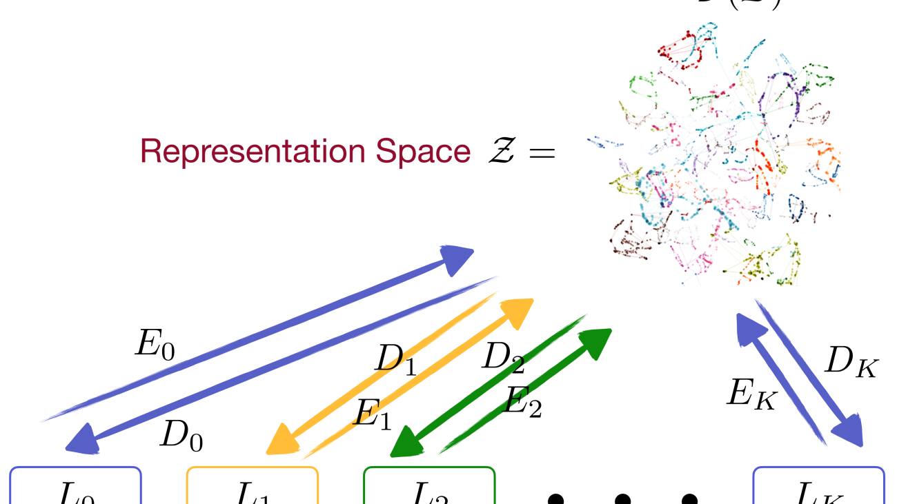
Figure 1: An encoder-decoder generative model of translation pairs, which helps to circumvent the limitation discussed before. There is a global distribution (mathcal{D}) over the representation space (mathcal{Z}), from which sentences of language (L_i) are generated via decoder (D_i). Similarly, sentences could also be encoded via (E_i) to (mathcal{Z}).

Despite the recent improvements in neural machine translation (NMT), training a large NMT model with hundreds of millions of parameters usually requires a collection of parallel corpora at a large scale, on the order of millions or even billions of aligned sentences for supervised training (Arivazhagan et al.). While it might be possible to automatically crawl the web to collect parallel sentences for high-resource language pairs, such as German-English and French-English, it is often infeasible or expensive to manually translate large amounts of sentences for low-resource language pairs, such as Nepali-English, Sinhala-English, etc. To this end, the goal of the so-called multilingual universal machine translation, a.k.a., universal machine translation (UMT), is to learn to translate between any pair of languages using a single system, given pairs of translated documents for some of these languages. The hope is that by learning a shared “semantic space” between multiple source and target languages, the model can leverage language-invariant structure from high-resource translation pairs to transfer to the translation between low-resource language pairs, or even enable zero-shot translation.

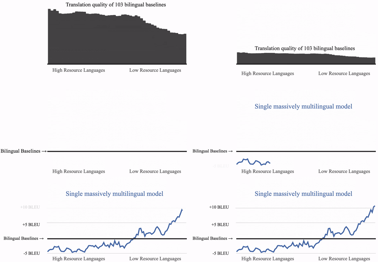
Indeed, training such a single massively multilingual model has gained impressive empirical results, especially in the case of low-resource language pairs (see Fig. 2). However, such success also comes with a cost. From Fig. 2 we observe that the translation quality over high-resource language pairs by using such a single UMT system is worse than the corresponding bilingual baselines.

Figure 2: Translation quality by using a single massively multilingual model against bilingual baselines that are trained for each one of the 103 language pairs. While the translation performances over low resource languages increase, the performances over high resource languages decrease. Our work provides a theoretical explanation for this empirical phenomenon. Figure credit: Exploring Massively Multilingual, Massive Neural Machine Translation.

Is this empirical phenomenon by coincidence? If not, why does it happen? Furthermore, what kind of structural assumptions about languages could help us get over this detrimental effect? In this blog post, based on our recent ICML paper, we take the first step towards understanding universal machine translation by providing answers to the above questions. The key takeaways of this blog post could be summarized as follows:

  • In a completely assumption-free setup, based on a common shared representation, no matter what decoder is used to translate the target languages, it is impossible to avoid making a large translation error on at least one pair of the translation pairs.
  • Under a natural generative model assumption for the data, after seeing aligned sentences for a linear number of language pairs (instead of quadratic!), we can learn encoder/decoders that perform well on any unseen language pair, i.e., zero-shot translation is possible.

An Impossibility Theorem on UMT via Language-Invariant Representations

Suppose we have an unlimited amount of parallel sentences for each pair of languages, with unbounded computational resources. Could we train a single model that performs well on all pairs of translation tasks based on a common representation space? Put it in other words, is there any information-theoretic limit of such systems for the task of UMT? In this paragraph we will show that there is an inherent tradeoff between the translation quality and the degree of representation invariance w.r.t. languages: the better the language invariance, the higher the cost on at least one of the translation pairs. At a high-level, this result holds due to the general data-processing principle: if a representation is invariant to multiple source languages, then any decoder based on this representation will have to generate the same language model on the target language. But on the other hand, the parallel corpora we use to train such a system could have drastically different sentence distributions on the target language, thus leading to a discrepancy (error) between the generated sentence distribution and the ground-truth sentence distribution over the target language.

To keep our discussions simple and transparent, let’s start with a basic Two-to-One setup where there are only two source languages (L_0) and (L_1) and one target language (L). Furthermore, for each source language (L_i, iin{0, 1}), let’s assume that there is a perfect translator (f_{L_ito L}^*) that takes a sentence (or string, sequence) from (L_i) and outputs the corresponding translation in (L). Under this setup, it is easy to see that there exists a perfect translator (f_L^*) in this Two-to-One task: $$f_L^*(x) = sum_{iin{0, 1}}mathbb{I}(xin L_i)cdot f_{L_ito L}^*(x)$$ In words: upon receiving a sentence (x), (f_L^*) simply checks which source language (x) comes from and then call the corresponding ground-truth translator.

To make the idea of language-invariant representations formal, let (g: Sigma^*to mathcal{Z}) be an encoder that takes a sentence (string) from alphabet (Sigma) to a representation in a vector space (mathcal{Z}). We call (g) an (epsilon)-universal language mapping if the distributions of sentence representations from different languages (L_0) and (L_1) are (epsilon)-close to each other. In words, (d(g_sharpmathcal{D}_0, g_sharpmathcal{D}_1)leq epsilon) for some divergence measure (d), where (g_sharpmathcal{D}_i) is the induced distribution of sentence (from (L_i)) representations in the shared space (mathcal{Z}). Subsequently, a multilingual system will train a decoder (h) that takes a sentence representation (z) and outputs the corresponding target translation in language (L). The hope here is that (z) encodes the language-invariant semantic information about the input sentence (either from (L_0) or from (L_1)) based on which to translate to the target language (L).

So far so good, but could we recover the perfect translator (f_L^*) by learning a common, shared representation (Z), i.e., (epsilon) is small? Unfortunately, the answer here is negative if we don’t have any assumption on the parallel corpora we use to train our encoder (g) and decoder (h):

Theorem (informal): Let (g:Sigma^*tomathcal{Z}) be an (epsilon)-universal language mapping. Then for any decoder (h:mathcal{Z}to Sigma_L^*), the following lower bound holds: $$text{Err}_{mathcal{D}_0}^{L_0to L}(hcirc g) + text{Err}_{mathcal{D}_1}^{L_1to L}(hcirc g)geq d(mathcal{D}_0(L), mathcal{D}_1(L))- epsilon.$$

Here the error term (text{Err}_{mathcal{D}_i}^{L_ito L}(hcirc g)) measures the (0-1) translation performance given by the encoder-decoder pair (hcirc g) from (L_i) to (L) over distribution (mathcal{D}_i). The first term (d(mathcal{D}_0(L), mathcal{D}_1(L))) in the lower bound measures the difference of distributions over sentences from the target language in the two parallel corpora, i.e., (L_0-L) and (L_1 – L). For example, in many practical scenarios, it may happen that the parallel corpus of high-resource language pair, e.g., German-English, contains sentences over a diverse domain whereas as a comparison, the parallel corpus of low-resource language pair, e.g., Sinhala-English, only contains target translations from a specific domain, e.g., sports, news, product reviews, etc. In this case, despite the fact that the target is the same language (L), the corresponding sentence distributions from English are quite different between different corpora, leading to a large lower bound. As a result, our theorem, which could be interpreted as a kind of uncertainty principle in UMT, says that no matter what kind of decoder we are going to use, it has to incur a large error on at least one of the translation pairs. It is also worth pointing out that our lower bound is algorithm-independent and it holds even with unbounded computation and data. As a final note, realize that for fixed distributions (mathcal{D}_i, iin{0, 1}), the smaller the (epsilon) (hence the better the language-invariant representations), the larger the lower bound, demonstrating an inherent tradeoff between language-invariance and translation performance in general.

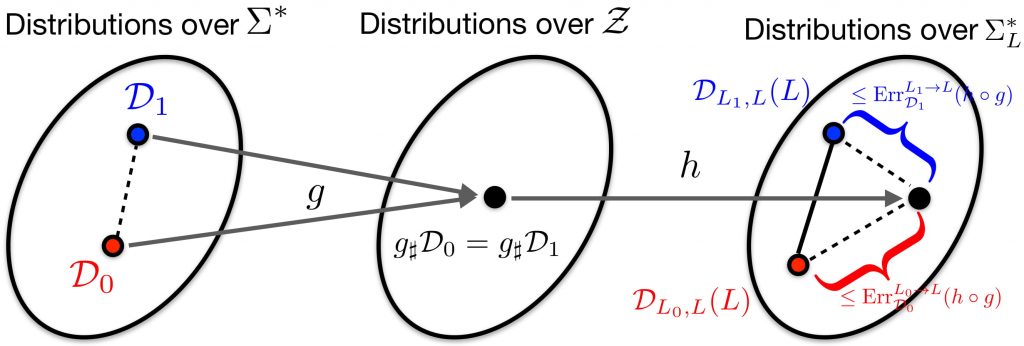
Proof Sketch: Here we provide a proof-by-picture (Fig. 3) in the special case of perfectly language-invariant representations, i.e., (epsilon = 0), to highlight the main idea in our proof of the above impossibility theorem. Please refer to our paper for more detailed proof as well as an extension of the above impossibility theorem in the more general many-to-many translation setting.

Figure 3: Proof by picture: Language-invariant representation (g) induces the same feature distribution over (mathcal{Z}), which leads to the same output distribution over the target language (Sigma_L^*). However, the parallel corpora of the two translation tasks in general have different marginal distributions over the target language, hence a triangle inequality over the output distributions gives the desired lower bound.

How can we Bypass this Limitation?

One way is to allow the decoder (h) to have access to the input sentences (besides the language-invariant representations) during the decoding process — e.g. via an attention mechanism on the input level. Technically, such information flow from input sentences during decoding would break the Markov structure of “input-representation-output” in Fig. 3, which is an essential ingredient in the proof of our theorem. Intuitively, in this case both language-invariant (hence language-independent) and language-dependent information would be used.

Another way would be to assume extra structure on the distributions of our corpora (mathcal{D}_{i}), i.e., by assuming some natural generative process capturing the distribution of the parallel corpora that are used for training. Since languages share a lot of semantic and syntactic characteristics, this would make a lot of sense — and intuitively, this is what universal translation approaches are banking on. In the next paragraph, we will do exactly this — we will show that under a suitable generative model, not only will there be a language-invariant representation, but it will be learnable using corpora from a very small (linear) number of pairs of language.

A Generative Model for UMT: A Linear Number of Translation Pairs Suffices!

In this section we will discuss a generative model, under which not only will there be a language-invariant representation, but it will be learnable using corpora from a very small (linear) number of pairs of language. Note that there are a quadratic number of translation pairs in our universe, hence our result shows that under this generative model zero-shot translation is actually possible.

To start with, what kind of generative model is suitable for the task of UMT? Ideally, we would like to have a feature space where vectors correspond to the semantic encoding of sentences from different languages. One could also understand it as a sort of “meaning” space. Then, language-dependent decoders would take these semantic vectors and decode them as the observable sentences. Figure 1 illustrates the generative process of our model, where we assume there is a common distribution (mathcal{D}) over the feature space (mathcal{Z}), from which parallel sentences are sampled and generated.

For ease of presentation, let’s first assume that each encoder-decoder pair ((E_i, D_i)) consists of deterministic mappings (see our paper on extensions with randomized encoders/decoders). The first question to ask is: how does this generative model assumption circumvent our previous lower bound in the last paragraph? We can easily observe that under the encoder-decoder generative assumption in Figure 1, the first term in our lower bound, (d(mathcal{D}_0(L), mathcal{D}_1(L))), gracefully reduces to 0, hence even if we try to learn perfectly language-invariant representations ((epsilon = 0)), there will be no loss of translation accuracy using universal language mapping. Perhaps what’s more interesting is that, under proper assumptions on the structure of (mathcal{F}), the class of encoders and decoders we learn from, by using the traditional empirical risk minimization (ERM) framework to learn the language-dependent encoders and decoders on a small number of language pairs, we could expect the learned encoders/decoders to well generalize on unseen language pairs as well! Informally,

Theorem (informal): Let (H) be a connected graph where each node (L_i) corresponds to a language and each edge ((L_i, L_j)) means that the learner has been trained on language pair (L_i) and (L_j), with empirical translation error (epsilon_{i,j}) and corpus of size (Omega(1 / epsilon_{i,j}^2 cdot log C(mathcal{F}))). Then with high probability, for any pair of language (L) and (L’) that are connected by a path (L = L_0, L_1, ldots, L_m = L’) in (H), its population level translation error is upper bounded by (O(sum_{k=0}^{m-1}epsilon_{k,k+1})).

In the theorem above, (C(mathcal{F})) is some complexity measure of the class (mathcal{F}). If we slightly simplify the theorem above by defining (epsilon := max_{(L_i, L_j)in H}epsilon_{i,j}) and realizing that the path length (m) is upper bounded by the diameter of the graph (H), (text{diam}(H)), we immediately obtain the following intuitive result:

For any pair of languages (L, L’) (the parallel corpus between (L) and (L’) may not necessarily appear in our training corpora), the translation error between (L) and (L’) is upper bounded by (O(text{diam}(H) cdot epsilon)).

The above corollary says that graphs (H) that do not have long paths are preferable. For example, (H) could be a star graph, where a central (high-resource) language acts as a pivot node. The proof of the theorem above essentially boils down to two steps: first, we use an epsilon-net argument to show that the learned encoders/decoders generalize on a pair of language that appears in our training corpora, and then by using the connectivity of the graph (H), we apply a chain of triangle-like inequalities to bound the error along the path connecting any pair of languages.

Some Concluding Thoughts

The prospect of building a single system for universal machine translation is appealing. Compared with building a quadratic number of bilingual translators, such a single system is easier to train, build, deploy, and maintain. More importantly, this could potentially allow the system to transfer some common knowledge in translation from high-resource languages to low-resource ones. However, such promise often comes with a price, which calls for proper assumptions on the generative process of the parallel corpora used for training. Our paper takes a first step towards better understanding the tradeoff in this regard and proposes a simple setup that allows for zero-shot translation. On the other hand, there are still some gaps between theory and practice. For example, it would be interesting to see whether the BLEU score, a metric used in the empirical evaluation of translation quality, bears a similar kind of lower bound. Also, could we further extend our generative modeling of sentences so that there are more hierarchical structures in the semantic space (mathcal{Z})? Empirically, it would be interesting to implement the above generative model on synthetic data to see the actual performance of zero-shot translation under the model assumption. These challenging problems (and more) will require collaborative efforts from a wide range of research communities and we hope our initial efforts could inspire more efforts in bridging the gap.

Reference

  1. Massively Multilingual Neural Machine Translation in the Wild: Findings and Challenges, Arivazhagan et al., https://arxiv.org/abs/1907.05019.
  2. Investigating Multilingual NMT Representations at Scale, Kudugunta et al., EMNLP 2019, https://arxiv.org/abs/1909.02197.
  3. On Learning Language-Invariant Representations for Universal Machine Translation, Zhao et al., ICML 2020, https://arxiv.org/abs/2008.04510.
  4. The Source-Target Domain Mismatch Problem in Machine Translation, Shen et al., https://arxiv.org/abs/1909.13151.
  5. How multilingual is Multilingual BERT? Pires et al., ACL 2019, https://arxiv.org/abs/1906.01502.

DISCLAIMER: All opinions expressed in this post are those of the author and do not represent the views of CMU.

Read More

Arcanum makes Hungarian heritage accessible with Amazon Rekognition

Arcanum makes Hungarian heritage accessible with Amazon Rekognition

Arcanum specializes in digitizing Hungarian language content, including newspapers, books, maps, and art. With over 30 years of experience, Arcanum serves more than 30,000 global subscribers with access to Hungarian culture, history, and heritage.

Amazon Rekognition Solutions Architects worked with Arcanum to add highly scalable image analysis to Hungaricana, a free service provided by Arcanum, which enables you to search and explore Hungarian cultural heritage, including 600,000 faces over 500,000 images. For example, you can find historical works by author Mór Jókai or photos on topics like weddings. The Arcanum team chose Amazon Rekognition to free valuable staff from time and cost-intensive manual labeling, and improved label accuracy to make 200,000 previously unsearchable images (approximately 40% of image inventory), available to users.

Amazon Rekognition makes it easy to add image and video analysis to your applications using highly scalable machine learning (ML) technology that requires no previous ML expertise to use. Amazon Rekognition also provides highly accurate facial recognition and facial search capabilities to detect, analyze, and compare faces.

Arcanum uses this facial recognition feature in their image database services to help you find particular people in Arcanum’s articles. This post discusses their challenges and why they chose Amazon Rekognition as their solution.

Automated image labeling challenges

Arcanum dedicated a team of three people to start tagging and labeling content for Hungaricana. The team quickly learned that they would need to invest more than 3 months of time-consuming and repetitive human labor to provide accurate search capabilities to their customers. Considering the size of the team and scope of the existing project, Arcanum needed a better solution that would automate image and object labelling at scale.

Automated image labeling solutions

To speed up and automate image labeling, Arcanum turned to Amazon Rekognition to enable users to search photos by keywords (for example, type of historic event, place name, or a person relevant to Hungarian history).

For the Hungaricana project, preprocessing all the images was challenging. Arcanum ran a TensorFlow face search across all 28 million pages on a machine with 8 GPUs in their own offices to extract only faces from images.

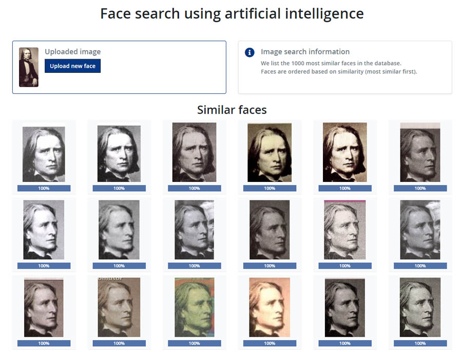
The following screenshot shows what an extract looks like (image provided by Arcanum Database Ltd).

The images containing only faces are sent to Amazon Rekognition, invoking the IndexFaces operation to add a face to the collection. For each face that is detected in the specified face collection, Amazon Rekognition extracts facial features into a feature vector and stores it in an Amazon Aurora database. Amazon Rekognition uses feature vectors when it performs face match and search operations using the SearchFaces and SearchFacesByImage operations.

The image preprocessing helped create a very efficient and cost-effective way to index faces. The following diagram summarizes the preprocessing workflow.

As for the web application, the workflow starts with a Hungaricana user making a face search request. The following diagram illustrates the application workflow.

The workflow includes the following steps:

  1. The user requests a facial match by uploading the image. The web request is automatically distributed by the Elastic Load Balancer to the webserver fleet.
  2. Amazon Elastic Compute Cloud (Amazon EC2) powers application servers that handle the user request.
  3. The uploaded image is stored in Amazon Simple Storage Service (Amazon S3).
  4. Amazon Rekognition indexes the face and runs SearchFaces to look for a face similar to the new face ID.
  5. The output of the search face by image operation is stored in Amazon ElastiCache, a fully managed in-memory data store.
  6. The metadata of the indexed faces are stored in an Aurora relational database built for the cloud.
  7. The resulting face thumbnails are served to the customer via the fast content-delivery network (CDN) service Amazon CloudFront.

Experimenting and live testing Hungaricana

During our test of Hungaricana, the application performed extremely well. The searches not only correctly identified people, but also provided links to all publications and sources in Arcanum’s privately owned database where found faces are present. For example, the following screenshot shows the result of the famous composer and pianist Franz Liszt.

The application provided 42 pages of 6×4 results. The results are capped to 1,000. The 100% scores are the confidence scores returned by Amazon Rekognition and are rounded up to whole numbers.

The application of Hungaricana has always promptly, and with a high degree of certainty, presented results and links to all corresponding publications.

Business results

By introducing Amazon Rekognition into their workflow, Arcanum enabled a better customer experience, including building family trees, searching for historical figures, and researching historical places and events.

The concept of face searching using artificial intelligence certainly isn’t new. But Hungaricana uses it in a very creative, unique way.

Amazon Rekognition allowed Arcanum to realize three distinct advantages:

  • Time savings – The time to market speed increased dramatically. Now, instead of spending several months of intense manual labor to label all the images, the company can do this job in a few days. Before, basic labeling on 150,000 images took months for three people to complete.
  • Cost savings – Arcanum saved around $15,000 on the Hungaricana project. Before using Amazon Rekognition, there was no automation, so a human workforce had to scan all the images. Now, employees can shift their focus to other high-value tasks.
  • Improved accuracy – Users now have a much better experience regarding hit rates. Since Arcanum started using Amazon Rekognition, the number of hits has doubled. Before, out of 500,000 images, about 200,000 weren’t searchable. But with Amazon Rekognition, search is now possible for all 500,000 images.

 “Amazon Rekognition made Hungarian culture, history, and heritage more accessible to the world,” says Előd Biszak, Arcanum CEO. “It has made research a lot easier for customers building family trees, searching for historical figures, and researching historical places and events. We cannot wait to see what the future of artificial intelligence has to offer to enrich our content further.”

Conclusion

In this post, you learned how to add highly scalable face and image analysis to an enterprise-level image gallery to improve label accuracy, reduce costs, and save time.

You can test Amazon Rekognition features such as facial analysis, face comparison, or celebrity recognition on images specific to your use case on the Amazon Rekognition console.

For video presentations and tutorials, see Getting Started with Amazon Rekognition. For more information about Amazon Rekognition, see Amazon Rekognition Documentation.


About the Authors

Siniša Mikašinović is a Senior Solutions Architect at AWS Luxembourg, covering Central and Eastern Europe—a region full of opportunities, talented and innovative developers, ISVs, and startups. He helps customers adopt AWS services as well as acquire new skills, learn best practices, and succeed globally with the power of AWS. His areas of expertise are Game Tech and Microsoft on AWS. Siniša is a PowerShell enthusiast, a gamer, and a father of a small and very loud boy. He flies under the flags of Croatia and Serbia.


Cameron Peron is Senior Marketing Manager for AWS Amazon Rekognition and the AWS AI/ML community. He evangelizes how AI/ML innovation solves complex challenges facing community, enterprise, and startups alike. Out of the office, he enjoys staying active with kettlebell-sport, spending time with his family and friends, and is an avid fan of Euro-league basketball.

Read More