Rethinking Attention with Performers

Rethinking Attention with Performers

Posted by Krzysztof Choromanski and Lucy Colwell, Research Scientists, Google Research

Transformer models have achieved state-of-the-art results across a diverse range of domains, including natural language, conversation, images, and even music. The core block of every Transformer architecture is the attention module, which computes similarity scores for all pairs of positions in an input sequence. This however, scales poorly with the length of the input sequence, requiring quadratic computation time to produce all similarity scores, as well as quadratic memory size to construct a matrix to store these scores.

For applications where long-range attention is needed, several fast and more space-efficient proxies have been proposed such as memory caching techniques, but a far more common way is to rely on sparse attention. Sparse attention reduces computation time and the memory requirements of the attention mechanism by computing a limited selection of similarity scores from a sequence rather than all possible pairs, resulting in a sparse matrix rather than a full matrix. These sparse entries may be manually proposed, found via optimization methods, learned, or even randomized, as demonstrated by such methods as Sparse Transformers, Longformers, Routing Transformers, Reformers, and Big Bird. Since sparse matrices can also be represented by graphs and edges, sparsification methods are also motivated by the graph neural network literature, with specific relationships to attention outlined in Graph Attention Networks. Such sparsity-based architectures usually require additional layers to implicitly produce a full attention mechanism.

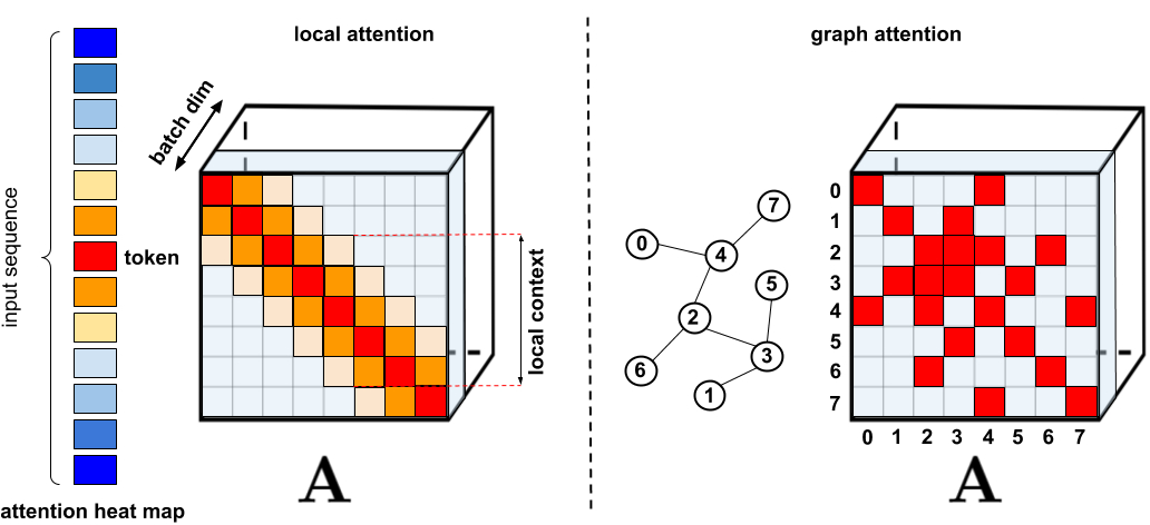
Standard sparsification techniques. Left: Example of a sparsity pattern, where tokens attend only to other nearby tokens. Right: In Graph Attention Networks, tokens attend only to their neighbors in the graph, which should have higher relevance than other nodes. See Efficient Transformers: A Survey for a comprehensive categorization of various methods.

Unfortunately, sparse attention methods can still suffer from a number of limitations. (1) They require efficient sparse-matrix multiplication operations, which are not available on all accelerators; (2) they usually do not provide rigorous theoretical guarantees for their representation power; (3) they are optimized primarily for Transformer models and generative pre-training; and (4) they usually stack more attention layers to compensate for sparse representations, making them difficult to use with other pre-trained models, thus requiring retraining and significant energy consumption. In addition to these shortcomings, sparse attention mechanisms are often still not sufficient to address the full range of problems to which regular attention methods are applied, such as Pointer Networks. There are also some operations that cannot be sparsified, such as the commonly used softmax operation, which normalizes similarity scores in the attention mechanism and is used heavily in industry-scale recommender systems.

To resolve these issues, we introduce the Performer, a Transformer architecture with attention mechanisms that scale linearly, thus enabling faster training while allowing the model to process longer lengths, as required for certain image datasets such as ImageNet64 and text datasets such as PG-19. The Performer uses an efficient (linear) generalized attention framework, which allows a broad class of attention mechanisms based on different similarity measures (kernels). The framework is implemented by our novel Fast Attention Via Positive Orthogonal Random Features (FAVOR+) algorithm, which provides scalable low-variance and unbiased estimation of attention mechanisms that can be expressed by random feature map decompositions (in particular, regular softmax-attention). We obtain strong accuracy guarantees for this method while preserving linear space and time complexity, which can also be applied to standalone softmax operations.

Generalized Attention
In the original attention mechanism, the query and key inputs, corresponding respectively to rows and columns of a matrix, are multiplied together and passed through a softmax operation to form an attention matrix, which stores the similarity scores. Note that in this method, one cannot decompose the query-key product back into its original query and key components after passing it into the nonlinear softmax operation. However, it is possible to decompose the attention matrix back to a product of random nonlinear functions of the original queries and keys, otherwise known as random features, which allows one to encode the similarity information in a more efficient manner.

LHS: The standard attention matrix, which contains all similarity scores for every pair of entries, formed by a softmax operation on the query and keys, denoted by q and k. RHS: The standard attention matrix can be approximated via lower-rank randomized matrices Q′ and K′ with rows encoding potentially randomized nonlinear functions of the original queries/keys. For the regular softmax-attention, the transformation is very compact and involves an exponential function as well as random Gaussian projections.

Regular softmax-attention can be seen as a special case with these nonlinear functions defined by exponential functions and Gaussian projections. Note that we can also reason inversely, by implementing more general nonlinear functions first, implicitly defining other types of similarity measures, or kernels, on the query-key product. We frame this as generalized attention, based on earlier work in kernel methods. Although for most kernels, closed-form formulae do not exist, our mechanism can still be applied since it does not rely on them.

To the best of our knowledge, we are the first to show that any attention matrix can be effectively approximated in downstream Transformer-applications using random features. The novel mechanism enabling this is the use of positive random features, i.e., positive-valued nonlinear functions of the original queries and keys, which prove to be crucial for avoiding instabilities during training and provide more accurate approximation of the regular softmax attention mechanism.

Towards FAVOR: Fast Attention via Matrix Associativity
The decomposition described above allows one to store the implicit attention matrix with linear, rather than quadratic, memory complexity. One can also obtain a linear time attention mechanism using this decomposition. While the original attention mechanism multiplies the stored attention matrix with the value input to obtain the final result, after decomposing the attention matrix, one can rearrange matrix multiplications to approximate the result of the regular attention mechanism, without explicitly constructing the quadratic-sized attention matrix. This ultimately leads to FAVOR+.

Left: Standard attention module computation, where the final desired result is computed by performing a matrix multiplication with the attention matrix A and value tensor V. Right: By decoupling matrices Q′ and K′ used in lower rank decomposition of A and conducting matrix multiplications in the order indicated by dashed-boxes, we obtain a linear attention mechanism, never explicitly constructing A or its approximation.

The above analysis is relevant for so-called bidirectional attention, i.e., non-causal attention where there is no notion of past and future. For unidirectional (causal) attention, where tokens do not attend to other tokens appearing later in the input sequence, we slightly modify the approach to use prefix-sum computations, which only store running totals of matrix computations rather than storing an explicit lower-triangular regular attention matrix.

Left: Standard unidirectional attention requires masking the attention matrix to obtain its lower-triangular part. Right: Unbiased approximation on the LHS can be obtained via a prefix-sum mechanism, where the prefix-sum of the outer-products of random feature maps for keys and value vectors is built on the fly and left-multiplied by query random feature vector to obtain the new row in the resulting matrix.

Properties
We first benchmark the space- and time-complexity of the Performer and show that the attention speedups and memory reductions are empirically nearly optimal, i.e., very close to simply not using an attention mechanism at all in the model.

Bidirectional timing for the regular Transformer model in log-log plot with time (T) and length (L). Lines end at the limit of GPU memory. The black line (X) denotes the maximum possible memory compression and speedups when using a “dummy” attention block, which essentially bypasses attention calculations and demonstrates the maximum possible efficiency of the model. The Performer model is nearly able to reach this optimal performance in the attention component.

We further show that the Performer, using our unbiased softmax approximation, is backwards compatible with pretrained Transformer models after a bit of fine-tuning, which could potentially lower energy costs by improving inference speed, without having to fully retrain pre-existing models.

Using the One Billion Word Benchmark (LM1B) dataset, we transferred the original pre-trained Transformer weights to the Performer model, which produces an initial non-zero 0.07 accuracy (dotted orange line). Once fine-tuned however, the Performer quickly recovers accuracy in a small fraction of the original number of gradient steps.

Example Application: Protein Modeling
Proteins are large molecules with complex 3D structures and specific functions that are essential to life. Like words, proteins are specified as linear sequences where each character is one of 20 amino acid building blocks. Applying Transformers to large unlabeled corpora of protein sequences (e.g. UniRef) yields models that can be used to make accurate predictions about the folded, functional macromolecule. Performer-ReLU (which uses ReLU-based attention, an instance of generalized attention that is different from softmax) performs strongly at modeling protein sequence data, while Performer-Softmax matches the performance of the Transformer, as predicted by our theoretical results.

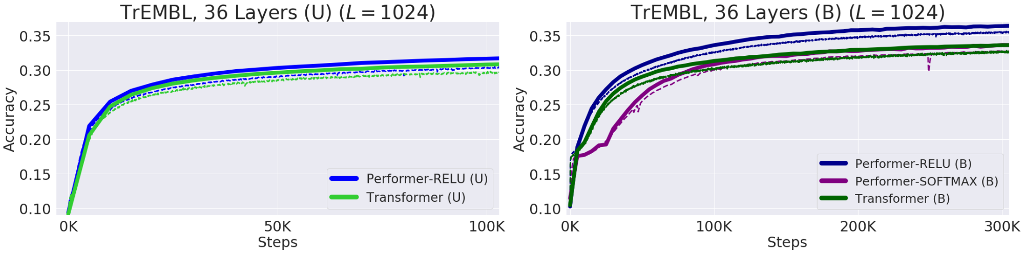
Performance at modeling protein sequences. Train = Dashed, Validation = Solid, Unidirectional = (U), Bidirectional = (B). We use the 36-layer model parameters from ProGen (2019) for all runs, each using a 16×16 TPU-v2. Batch sizes were maximized for each run, given the corresponding compute constraints.

Below we visualize a protein Performer model, trained using the ReLU-based approximate attention mechanism. Using the Performer to estimate similarity between amino acids recovers similar structure to well-known substitution matrices obtained by analyzing evolutionary substitution patterns across carefully curated sequence alignments. More generally, we find local and global attention patterns consistent with Transformer models trained on protein data. The dense attention approximation of the Performer has the potential to capture global interactions across multiple protein sequences. As a proof of concept, we train models on long concatenated protein sequences, which overloads the memory of a regular Transformer model, but not the Performer due to its space efficiency.

Left: Amino acid similarity matrix estimated from attention weights. The model recognizes highly similar amino acid pairs such as (D,E) and (F,Y), despite only having access to protein sequences without prior information about biochemistry. Center: Attention matrices from 4 layers (rows) and 3 selected heads (columns) for the BPT1_BOVIN protein, showing local and global attention patterns.
Performance on sequences up to length 8192 obtained by concatenating individual protein sequences. To fit into TPU memory, the Transformer’s size (number of layers and embedding dimensions) was reduced.

Conclusion
Our work contributes to the recent efforts on non-sparsity based methods and kernel-based interpretations of Transformers. Our method is interoperable with other techniques like reversible layers and we have even integrated FAVOR with the Reformer’s code. We provide the links for the paper, Performer code, and the Protein Language Modeling code. We believe that our research opens up a brand new way of thinking about attention, Transformer architectures, and even kernel methods.

Acknowledgements
This work was performed by the core Performers designers Krzysztof Choromanski (Google Brain Team, Tech and Research Lead), Valerii Likhosherstov (University of Cambridge) and Xingyou Song (Google Brain Team), with contributions from David Dohan, Andreea Gane, Tamas Sarlos, Peter Hawkins, Jared Davis, Afroz Mohiuddin, Lukasz Kaiser, David Belanger, Lucy Colwell, and Adrian Weller. We give special thanks to the Applied Science Team for jointly leading the research effort on applying efficient Transformer architectures to protein sequence data.

We additionally wish to thank Joshua Meier, John Platt, and Tom Weingarten for many fruitful discussions on biological data and useful comments on this draft, along with Yi Tay and Mostafa Dehghani for discussions on comparing baselines. We further thank Nikita Kitaev and Wojciech Gajewski for multiple discussions on the Reformer, and Aurko Roy and Ashish Vaswani for multiple discussions on the Routing Transformer.

Read More

Government Execs Must Be ‘Brave, Bold and Benevolent’ to Hasten AI Adoption, Experts Say

Government Execs Must Be ‘Brave, Bold and Benevolent’ to Hasten AI Adoption, Experts Say

Hundreds of technology experts from the public and private sectors, as well as academia, came together earlier this month for NVIDIA’s GPU Technology Conference to discuss U.S. federal agency adoption of AI and how industry can help.

Leaders from dozens of organizations, including the U.S. Department of Defense, the Federal Communication Commission, Booz Allen Hamilton, Lockheed Martin, NASA, RAND Corporation, Carnegie Mellon and Stanford Universities, participated in approximately 100 sessions that were part of GTC’s Public Sector Summit.

They talked about the need to accelerate efforts in a number of areas, including education, access to data and computing resources, funding and research. Many encouraged government executives and federal agencies to act with a greater sense of urgency.

“Artificial intelligence is inspiring the greatest technological transformation of our time,” Anthony Robbins, vice president of federal at NVIDIA, said in a panel with former Federal CIO Suzette Kent and retired Lt. Gen. Jack Shanahan during one of the talks focused on “Building an AI Nation.” “The train has left the station,” Robbins said. “In fact, it’s already roaring down the tracks.”

“We’re in a critical period with the United States government,” Shanahan said during the panel. “We have to get it right. This is a really important conversation.”

Just Get Started

These and other speakers cited a common theme: agencies need to get started now. But this requires a cultural shift, which Kent spoke of as one of the most significant challenges she experienced as federal CIO.

“In any kind of transformation the tech is often the easy part,” she said, noting that the only way to get people on board across the U.S. government — one of the largest and most complex institutions in the world — is to focus on return on investment for agency missions.

In a session titled “Why Leaders in Both the Public and Private Sectors Should Embrace Exponential Changes in Data, AI, and Work,” David Bray, former Senior National Intelligence Service Executive, FCC CIO, and current inaugural director and founder of the GeoTech Center at the Atlantic Council, tackled the same topic, saying that worker buy-in was important not just for AI adoption but also for its sustainability.

“If you only treat this as a tech endeavor, you might get it right, but it won’t stick,” Bray said. “What you’re doing isn’t an add-on to agencies — this is transforming how the government does business.”

Make Data a Priority

Data strategy came up repeatedly as an important component to the future of federal AI.

Less than an hour before a GTC virtual fireside chat with Robbins and DoD Chief Data Officer David Spirk, the Pentagon released its first enterprise data strategy.

The document positions the DoD to become a data-centric organization, but implementing the strategy won’t be easy, Spirk said. It will require an incredible amount of orchestration among the numerous data pipelines flowing in and out of the Pentagon and its service branches.

“Data is a strategic asset,” he said. “It’s a high-interest commodity that has to be leveraged for both immediate and lasting advantage.”

Kent and Shanahan agreed that data is critical. Kent said agency chief data officers need to think of the federal government as one large enterprise with a huge repository of data rather than silos of information, considering how the government at large can leverage an agency’s data.

Invest in Exponential Change

The next few years will be crucial for the government’s adoption of AI, and experts say more investment will be needed.

To start, the government will have to address the AI talent gap. The exact extent of the talent shortage is difficult to measure, but job website statistics show that demand for workers far exceeds supply, according to a study by Georgetown University’s Center for Security and Emerging Technology.

One way to do that is for the federal government to set aside money to help small and mid-sized universities develop AI programs.

Another is to provide colleges and universities with access to more computing resources and federal datasets, according to John Etchemendy, co-director of the Human Centered Artificial Intelligence at Stanford University, who spoke during a session with panelists from academia and think tanks. That would accelerate R&D and help students become more proficient at data science.

Government investment in AI research will also be key in helping agencies move forward. Without a significant increase, the United States will fall behind, Martijn Rasser, senior fellow at the Center for New American Security, said during the panel discussion. CNAS recently released a report calling for $25 billion per year in federal AI investment by 2025.

The RAND Corp. released a congressionally mandated assessment of the DoD’s AI posture last year that recommended defense agencies need to create mechanisms for connecting AI researchers, technology developers and operators. By allowing operators to be part of the process at every stage, they’ll be more confident and trusting of the new technology, Danielle Tarraf, senior information scientist at RAND, told the panel. Tarraf highlighted that many of these recommendations were applicable government-wide.

Michael McQuade, vice president of research at Carnegie Mellon University and a member of the Defense Innovation Board, argued that it’s crucial that we start delivering solutions now. “Building confidence is key” to continue to justify the increasing support from authorizers and appropriators for the crucial national investments in Al.

By framing AI in the context of both broad AI innovations and individual use cases, government can elucidate why it’s so important to “knock down barriers and get the money in the right place,” said Seth Center, a senior advisor to the National Security Commission on AI.

An overarching theme from the Public Sector Summit was that government technology leaders need to heighten their focus on AI, with a sense of urgency.

Kent and Shanahan noted that training and tools are available for the government to make the transition smoothly, and begin using the technology. Both said that by partnering with industry and academia, the federal government can make an AI-equipped America a reality.

Bray, noting the breakneck pace of change from new technologies, said that it usually takes decades for the kind of shifts that are now possible. He urged government executives to take an active role in guiding those changes, encouraging them to be “brave, bold and benevolent.”

The post Government Execs Must Be ‘Brave, Bold and Benevolent’ to Hasten AI Adoption, Experts Say appeared first on The Official NVIDIA Blog.

Read More

Old Clips Become Big Hits: AI-Enhanced Videos Script a Success Story

Old Clips Become Big Hits: AI-Enhanced Videos Script a Success Story

After his AI-enhanced vintage video went viral, Denis Shiryaev launched a startup to bottle the magic. Soon anyone who wants to dust off their old films may be able to use his neural networks.

The story began with a blog on Telegram by the Russian entrepreneur currently living in Gdańsk, Poland.

“Some years ago I started to blog about machine learning and play with different algorithms to understand it better,” said Shiryaev, who later founded the startup known by its web address, neural.love. “I was generating music with neural nets and staging Turing tests of chatbots — silly, fun stuff.”

Eight months ago, he tried an AI experiment with a short, grainy film he’d found on YouTube of a train in 1896 arriving in a small French town. He used open-source software and AI models to upscale it to 4K resolution and smooth its jerky motion from 15 frames per second to 60 fps.

“I posted it one night, and when I woke up the next day, I had a million views and was on the front page of Reddit. My in-box was exploding with messages on Facebook, LinkedIn — everywhere,” he said of responses to the video below

Not wanting to be a one-hit wonder, he found other vintage videos to work with. He ran them through an expanding workflow of AI models, including DeOldify for adding color and other open-source algorithms for removing visual noise.

His inbox stayed full.

He got requests from a media company in the Netherlands to enhance an old film of Amsterdam. Displays in the Moscow subway played a vintage video he enhanced of the Russian capital. A Polish documentary maker knocked on his door, too.

Even the USA was calling. PBS asked for help with footage for an interactive website for its documentary on women’s suffrage.

“They had a colorist for the still images, but even with advances in digital painting, colorizing film takes a ridiculous amount of time,” said Elizabeth Peck, the business development manager for the five-person team at neural.love.

NVIDIA RTX Speeds AI Work 60x+

Along the way, Shiryaev and team got an upgrade to the latest NVIDIA RTX 6000 GPU. It could process 60 minutes of video in less time than an earlier graphics card took to handle 90 seconds of footage.

The RTX card also trains the team’s custom AI models in eight hours, a job that used to take a week.

“This card shines, it’s amazing how helpful the right hardware can be,” he said.

AI Film Editor in the Cloud

The bright lights the team sees these days are flashing images of a future consumer service in the public cloud. An online self-serve AI video editor could help anyone with a digital copy of an old VHS tape or Super8 reel in their closet.

“People were sending us really touching footage — the last video of their father, a snippet from a Michael Jackson concert they attended as a teenager. The amount of personal interest people had in what we were doing was striking,” explained Peck.

It’s still early days. Shiryaev expects it will take a few months to get a beta service ready for launch.

Meanwhile, neural.love is steering clear of the VC world. “We don’t want to take money until we are sure there is a market and we have a working product,” he said.

You can hear more of neural.love’s story in a webinar hosted by PNY Technologies, an NVIDIA partner.

The post Old Clips Become Big Hits: AI-Enhanced Videos Script a Success Story appeared first on The Official NVIDIA Blog.

Read More

What Is Computer Vision?

What Is Computer Vision?

Computer vision has become so good that the days of general managers screaming at umpires in baseball games in disputes over pitches may become a thing of the past.

That’s because developments in image classification along with parallel processing make it possible for computers to see a baseball whizzing by at 95 miles per hour. Pair that with image detection to help geolocate balls, and you’ve got a potent umpire tool that’s hard to argue with.

But computer vision doesn’t stop at baseball.

What Is Computer Vision?

Computer vision is a broad term for the work done with deep neural networks to develop human-like vision capabilities for applications, most often run on NVIDIA GPUs. It can include specific training of neural nets for segmentation, classification and detection using images and videos for data.

Major League Baseball is testing AI-assisted calls at the plate using computer vision. Judging balls and strikes on baseballs that can take just .4 seconds to reach the plate isn’t easy for human eyes. It could be better handled by a camera feed run on image nets and NVIDIA GPUs that can process split-second decisions at a rate of more than 60 frames per second.

Hawk-Eye, based in London, is making this a reality in sports. Hawk-Eye’s NVIDIA GPU-powered ball tracking and SMART software is deployed in more than 20 sports, including baseball, basketball, tennis, soccer, cricket, hockey and NASCAR.

Yet computer vision can do much more than just make sports calls.

What Is Computer Vision Beyond Sports?

Computer vision can handle many more tasks. Developed with convolutional neural networks, computer vision can perform segmentation, classification and detection for a myriad of applications.

Computer vision has infinite applications. With industry changes from computer vision spanning sports, automotive, agriculture, retail, banking, construction, insurance and beyond, much is at stake.

3 Things to Know About Computer Vision

  • Segmentation: Image segmentation is about classifying pixels to belong to a certain category, such as a car, road or pedestrian. It’s widely used in self-driving vehicle applications, including the NVIDIA DRIVE software stack, to show roads, cars and people.  Think of it as a sort of visualization technique that makes what computers do easier to understand for humans.
  • Classification: Image classification is used to determine what’s in an image. Neural networks can be trained to identify dogs or cats, for example, or many other things with a high degree of precision given sufficient data.
  • Detection: Image detection allows computers to localize where objects exist. It puts rectangular bounding boxes — like in the lower half of the image below — that fully contain the object. A detector might be trained to see where cars or people are within an image, for instance, as in the numbered boxes below.

What You Need to Know: Segmentation, Classification and Detection

Segmentation Classification Detection
Good at delineating objects Is it a cat or a dog? Where does it exist in space?
Used in self-driving vehicles Classifies with precision Recognizes things for safety


NVIDIA’s Deep Learning Institute offers courses such as Getting Started with Image Segmentation and Fundamentals of Deep Learning for Computer Vision

The post What Is Computer Vision? appeared first on The Official NVIDIA Blog.

Read More

From academia to industry: How Facebook Engineer Jason Flinn started his journey in Core Systems

Partnering with university faculty helps us drive impactful, innovative solutions to real-world technology challenges. From collaborations to funding research through requests for proposals, working with academia is important to our mission of giving people the power to build community and bringing the world closer together.

Many members of our Facebook research community come from long and accomplished careers in academia. One example is Jason Flinn, a former professor at the University of Michigan. After an extensive academic career in software systems, which recently earned him the prestigious Test of Time award, Flinn became a Software Engineer on Facebook’s Core Systems, a team that performs forward-looking research in the area of distributed systems and applies key systems architecture techniques at Facebook’s scale.

Flinn’s first industry collaboration with Facebook was with one of his PhD students, Mike Chow, who was a PhD intern at the time. This experience gave Flinn a preview of what it would be like to work in industry as a researcher. “I do my best work when I build systems that have real-world use,” he explains. “In my early career in mobile computing, I was the person using the system, and I learned the right research questions to ask from examining my own experiences. Today, with Core Systems, I have thousands of engineers using the systems that I am building, and I am learning the right research questions to ask from deploying these systems at scale.”

We sat down with Flinn to learn more about how he came to work at Facebook after a career in academia, the differences between industry and academia for someone in Core Systems, his current research projects, advice for those looking to follow a similar path, and more.

Q: Tell us about your experience in academia before joining Facebook.

Jason Flinn: Prior to joining Facebook, I was a professor at the University of Michigan for over two decades. My research interests over the years have been really varied. I’ve always enjoyed the opportunity afforded by computer science research to explore new topics and branch out into related subfields. My PhD dissertation looked at software power management and developed ways to extend the battery lifetime of mobile computers. I’ve returned to mobile computing throughout my career, developing distributed storage systems and investigating ways to improve wireless networking through better power management and strategic use of multiple networks. I also was fortunate to get involved in some of the earliest work in edge computing and vehicle-to-infrastructure networking. For another large part of my career, I studied topics in storage systems and distributed computing, including distributed file systems and software applications of speculative execution and deterministic replay.

Since joining Facebook, I have run into so many former students who now work for the company and have taken these classes with me. This has been a great reminder that one of the primary contributions to academia is our impact on the students we teach.

Q: What has your journey with Facebook been like so far?

JF: When I was at the University of Michigan, I participated in a couple of joint research projects with Facebook engineers. In both cases, the collaborations were kicked off by discussions with my former PhD students who had joined Facebook as full-time engineers. One of my then-PhD students, Mike Chow, joined Facebook for an extended nine-month internship, and we jointly developed a tool with Dan Peek (another former student), David Meisner, and Thomas Wenisch called the Mystery Machine. The key insight in this paper was that we could apply data at massive scale to learn the relationships and dependencies between execution points in software systems without needing to annotate or fully instrument such systems by hand.

This paper received a lot of visibility when it was published at OSDI, and has proved to be quite influential in showing the community the potential of applying machine learning and data at scale to software tracing and debugging. This collaboration was so successful that Mike did a subsequent internship with another of my PhD students, Kaushik Veeraraghavan, resulting in the DQBarge paper at OSDI 2016.

In 2018, I was eligible for a sabbatical and looking for a change of pace. I wound up talking to Mahesh Balakrishnan about the Delos project he had recently started at Facebook around the idea of virtualizing consensus through the use of a reconfigurable, distributed shared log. Delos offered me the chance to dive right in and design new, cutting-edge protocols, so I quickly jumped into this project. We were originally only a small team of four people, but within my first few months on the project, we were deploying our code at the heart of the Facebook control plane. After about nine months, I decided to join Facebook as a full-time employee.

Q: What are you currently working on?

JF: I’ve worked on two major projects at Facebook. The first is the Delos project mentioned above. Our team built a strongly consistent metadata store for Facebook control plane services like the container scheduler and resource allocation systems. Such systems are notoriously complex and fraught with peril to develop and deploy, often because they are a low-level building block on which all higher levels of the software stack depend.

One of the most fun parts of this project for me was when we deployed this new protocol in production for the first time. We executed a single command and the Delos virtualized architecture swapped an entire data center to the new protocol with zero downtime and no fuss. I don’t think anything like this had ever been done before, so it felt like quite an achievement to see it happen. The team has leveraged virtualized consensus in lots of different ways since then: for example, in deploying a point-in-time database restore capability, swapping protocols for Delos’s own internal metadata storage, and swapping between disaggregated and aggregated logs to help mitigate production issues.

My second project is called Hedwig. This project is unifying the delivery of large, hot data content to very large numbers of consumer machines distributed around the world. In academic research and in industry, there has been a lot of prior work on highly decentralized systems for delivering such content (BitTorrent is one example of a system in this space). Yet, with the deployment of public and private clouds, there is an opportunity to reexamine this space and look at how we can optimize such systems for a managed data center environment in which the system has greater visibility into network topology and resource availability, and in which we also have the opportunity to leverage highly-reliable, well-maintained centralized services.

Hedwig aims to achieve the best of both worlds by providing a simple, decentralized peer-to-peer data plane in combination with a well-managed, centralized control plane. Hedwig is also designed to be highly customizable through flexible policy modules in its centralized control plane. These policies let Hedwig employ different caching, routing, and failure handling policies for different use cases. In turn, this lets us easily optimize Hedwig for different workloads and services.

Q: What’s the difference between working in systems at Facebook versus in academia?

JF: I have always admired the industry papers that appeared in early SOSP conferences that described experiences building production software systems (Unix, AFS, etc.). What makes these papers great is that they not only contain big ideas, but they also combine these ideas with practical lessons and observations that come from deploying and using the systems. Reading the papers, I can feel how the deployment of the systems really helped the authors understand what was most important and innovative about their work (for example, the simplicity of the Unix interface, or the concept of scalability in the AFS paper that was decades ahead of its time).

Working in Core Systems gives me the opportunity to replicate some of the ingredients that helped make these papers so great. In academia, my focus was on writing papers and working with my students. My students and I built systems to validate our ideas, and together we might write several papers about a particular system as we were developing the ideas. At Facebook Core Systems, my focus has been first on building the systems, deploying them at scale, and learning from them. I can let the systems bake and evolve over time before writing a paper that describes what we did. This process leads to fewer papers, but I hope it also leads to stronger papers like the early industry papers I admire.

We followed this path with our Delos paper that’s appearing at OSDI this year, and I hope to take a similar approach to describing my current work on Hedwig.

Q: You recently earned a Test of Time award for your work in adaptable battery use in mobile apps. What influenced this research?

JF: It’s often said that asking the right questions is the hardest part of research, and I think this is especially true in this situation. It was all about being in the right place at the right time.

I was really fortunate to attend grad school at Carnegie Mellon when they had just deployed the first campus-wide wireless network. This gave me the opportunity to take my laptop outside and work with an actual internet connection. (Although hard to imagine today, this was incredibly novel at the time.) Almost the first thing I noticed was that my laptop battery would quickly die. This was the “aha!” moment — that reducing energy usage was going to be incredibly vital for any type of mobile computer. This led to all sorts of interesting questions: Can we measure energy usage and attribute that energy to the software running on the computer? What types of strategies can software employ to extend the battery lifetime of the computer? Can the operating system adapt the behavior of the software to optimize for energy savings or quality/performance?

Q: For someone in academia curious about collaborating with or working at Facebook, where would you recommend they start?

JF: My best collaborations (both with Facebook and elsewhere) have involved sending a student to work directly with industry teams for a period of time (i.e., an internship) or working directly on the project myself (e.g., on sabbatical or for a few hours every week). My Facebook collaborations started out with long conversations with Facebook engineers at conferences where we would kick a bunch of ideas around. The final project wound up in the same general area as these conversations, but it was really the process of embedding with a Facebook team that generated the best research directions.

Working with Facebook, there is a tremendous opportunity to collect real-world systems measurements at scale to validate ideas. It’s important to utilize this opportunity during any collaboration.

I also learned to budget some time after any internship or sabbatical to work on the idea in academia where one can build a smaller-scale replica, tweak, and measure the system in a way that is not possible in a production system. Combining these two styles of research can result in really strong work.

The post From academia to industry: How Facebook Engineer Jason Flinn started his journey in Core Systems appeared first on Facebook Research.

Read More

Securing Amazon SageMaker Studio connectivity using a private VPC

Securing Amazon SageMaker Studio connectivity using a private VPC

Amazon SageMaker Studio is the first fully integrated development environment (IDE) for machine learning (ML). With a single click, data scientists and developers can quickly spin up Amazon SageMaker Studio Notebooks for exploring datasets and building models. With the new ability to launch Amazon SageMaker Studio in your Amazon Virtual Private Cloud (Amazon VPC), you can control the data flow from your Amazon SageMaker Studio notebooks. This allows you to restrict internet access, monitor and inspect traffic using standard AWS networking and security capabilities, and connect to other AWS resources through AWS PrivateLink or VPC endpoints.

In this post, we explore how the Amazon SageMaker Studio VPC connectivity works, implement a sample architecture, and demonstrate some security controls in action.

Solution overview

When experimenting with and deploying ML workflows, you need access to multiple resources, such as libraries, packages, and datasets. If you’re in a highly regulated industry, controlling access to these resources is a paramount requirement. Amazon SageMaker Studio allows you to implement security in depth, with features such as data encryption, AWS Identity and Access Management (IAM), and AWS Single Sign-On (AWS SSO) integration. The ability to launch Amazon SageMaker Studio in your own private VPC adds another layer of security.

Amazon SageMaker Studio runs on an environment managed by AWS. When launching a new Studio domain, the parameter AppNetworkAccessType defines the external connectivity for such domain. Previously, the only option available for this parameter was DirectInternetOnly, meaning the traffic from the notebook flowed from an AWS managed internet gateway, as described in the following diagram.

The Amazon Elastic File System (Amazon EFS) volumes that store the Studio users’ home directories resides in the customer VPC, even when AppNetworkAccessType=DirectInternetOnly. You can optionally specify which VPC and subnet to use.

With the newly introduced feature to launch Studio in your VPC, you can set the AppNetworkAccessType parameter to VpcOnly. This launches Studio inside the specified VPC, communicating with the domain through an elastic network interface (ENI). You can apply security groups to that ENI to enforce a first layer of security control.

You can also use VPC endpoints to establish a private connection between the Studio domain and other AWS services, such as Amazon Simple Storage Service (Amazon S3) for data storage and Amazon CloudWatch for logging and monitoring, without requiring internet connectivity. VPC endpoints can impose additional networking controls such as VPC endpoint IAM policies that may, for example, only allow traffic to certain S3 buckets. The following diagram illustrates this architecture.

Prerequisites

Before getting started, make sure you have the following prerequisites:

  • An AWS account
  • An IAM user or role with administrative access
  • Curiosity 🙂

Setting up your environment

To better understand how the feature works, we provide an AWS CloudFormation template to set up a basic environment where you can experiment with Amazon SageMaker Studio running inside a VPC. After deployment, the environment looks like the following diagram.

This template deploys the following resources in your account:

  • A new VPC, with a private subnet and security group. Because communication occurs across multiple Studio resources, this security group applied to the Studio ENI should allow inbound traffic to itself.
  • An encrypted S3 bucket, with bucket policies restricting access to our S3 endpoint.
  • VPC endpoints with policies for access control:
    • We use an Amazon S3 endpoint to demonstrate the ability to limit traffic to specific S3 buckets.
    • Because Studio has its traffic routed through the VPC, access to supporting services needs to be provisioned through VPC endpoints. Amazon CloudWatch Logs allows Studio to push logs generated by the service. We need an Amazon SageMaker API endpoint to launch Studio notebooks, training jobs, processing jobs, and deploy endpoints, and an Amazon SageMaker RunTime endpoint for services to call the Amazon SageMaker inference endpoint.
  • An IAM execution role. This role is assigned to Amazon SageMaker and defines which access permissions Studio has.

To set up your environment, click on the link below. The template is also available at this GitHub repo.

Creating an Amazon SageMaker Studio domain inside a VPC

With the infrastructure in place, you’re ready to create an Amazon SageMaker Studio domain and assign it to a VPC.

For more information about the options available to set up Studio, see Onboard to Amazon SageMaker Studio. If you have an existing domain, you might want to delete it and recreate it, or create a separate one.

To create the domain, you can use the following:

To use the console to create a Studio domain and tie it to the VPC infrastructure deployed by the template, complete the following steps:

  1. On the Amazon SageMaker console, choose SageMaker Studio.

If you don’t have a domain created, a screen appears.

  1. For Get Started, select Standard setup.
  2. For Authentication method, select AWS Identity and Access Management (IAM).
  3. For Execution role for all users, choose your notebook IAM role (the default is studiovpc-notebook-role).
  4. In the Network section, for VPC, choose your VPC (the default is studiovpc-vpc).
  5. For Subnet, choose your subnet (the default is studiovpc-private-subnet).

Make sure to not choose studiovpc-endpoint-private-subnet.

  1. For Network Access for Studio, select VPC Only.

  1. Choose Submit.

To create and link the domain with the AWS CLI, enter the following code. The option --app-network-access-type VpcOnly links the domain to our VPC. The VPC and subnet parameters are set by the --default-user-settings option.

#Please replace the variable below according to your environment
REGION= #AWS Region where the Domain will be created
AWS_ACCOUNT_ID= #AWS Account ID 
VPC_DOMAIN_NAME= #Select a name for your Domain

#The values below can be obtained on the "Output" section of the CloudFormation used on the previous step
VPC_ID=
PRIVATE_SUBNET_IDS=
SECURITY_GROUP=
EXECUTION_ROLE_ARN=

#Now let's create the domain
aws sagemaker create-domain 
--region $REGION 
--domain-name $VPC_DOMAIN_NAME 
--vpc-id $VPC_ID 
--subnet-ids $PRIVATE_SUBNET_IDS 
--app-network-access-type VpcOnly 
--auth-mode IAM 
--default-user-settings "ExecutionRole=${EXECUTION_ROLE_ARN},SecurityGroups=${SECURITY_GROUP}"

#Please note the DomainArn output - we will use it on the next step

Creating a user profile

Now that the domain is created, we need to create a user profile. You can create multiple user profiles associated to a single domain.

To create your user profile on the console, complete the following steps:

  1. On the Amazon SageMaker Studio console, choose Control Panel.
  2. Choose Add user profile.
  3. For User name, enter a name (for example, demo-user).
  4. For Execution role, choose your IAM role (the default is studiovpc-notebook-role).

To create your user profile with the AWS CLI, enter the following code:

#Please replace the variable below according to your environment
DOMAIN_ID= #From previous step
USER_PROFILE_NAME= #Select a name for your user profile

#Now let's create the profile
aws sagemaker create-user-profile 
--region $REGION 
--domain-id $DOMAIN_ID 
--user-profile-name $USER_PROFILE_NAME

Accessing Amazon SageMaker Studio

We now have a Studio domain associated to our VPC and a user profile in this domain. Now we need to give access to the user. To do so, we create a pre-signed URL.

To use the console, on the Studio Control Panel, locate your user name and choose Open Studio.

To use the AWS CLI, enter the following code:

#Now let's create the pre-signed URL
aws sagemaker create-presigned-domain-url 
--region $REGION 
 --domain-id $DOMAIN_ID 
--user-profile-name $USER_PROFILE_NAME

#Please take note of the Domain URL, and paste it on a browser that have VPC Connectivity

At this point, our deployment looks like the following diagram.

We made it! Now you can use your browser to connect to the Amazon SageMaker Studio domain. After a few minutes, Studio finishes creating your environment and you’re greeted with the launcher screen (see the following screenshot).

Security controls

Some examples of security best practices are Amazon S3 access control and limiting internet ingress and egress. In this section, we see how to implement them in combination with running Amazon SageMaker Studio in a private VPC.

Amazon S3 access control

Developing ML models requires access to sensitive data stored on specific S3 buckets. You might want to implement controls to guarantee that:

  • Only specific Studio domains can access these buckets
  • Each Studio domain only have access to the defined S3 buckets

We can achieve this using the sample architecture provided in the CloudFormation template.

Our CloudFormation template created an S3 bucket with the following S3 bucket policy attached to it. The condition StringsNotEquals evaluates the VPC endpoint ID with the effect set to deny, meaning that access to the S3 bucket is denied if the access doesn’t come from the designated VPC endpoint. You can find your specific bucket name on the AWS CloudFormation console, on the Outputs tab for the stack.

{
    "Version": "2008-10-17",
    "Statement": [
        {
            "Effect": "Deny",
            "Principal": "*",
            "Action": [
                "s3:GetObject",
                "s3:PutObject",
                "s3:ListBucket"
            ],
            "Resource": [
                "arn:aws:s3:::<s3-bucket-name>/*",
                "arn:aws:s3:::<s3-bucket-name>"
            ],
            "Condition": {
                "StringNotEquals": {
                    "aws:sourceVpce": "<s3-vpc-endpoint-id>"
                }
            }
        }
    ]

The Amazon S3 VPC endpoint also has a policy attached to it. This policy only allows access to the S3 bucket created by AWS CloudFormation:

{
    "Version": "2012-10-17",
    "Statement": [
        {
            "Effect": "Allow",
            "Principal": "*",
            "Action": [
                "s3:GetObject",
                "s3:PutObject",
                "s3:ListBucket"
            ],
            "Resource": [
                "arn:aws:s3:::<s3-bucket-name>",
                "arn:aws:s3:::<s3-bucket-name>/*"
            ]
        }
    ]

This combination of S3 bucket policy and VPC endpoint policy, together with Studio VPC connectivity, establishes that Studio can only access the referenced S3 bucket, and this S3 bucket can only be accessed from the VPC endpoint.

To test it, open a notebook in Studio and try to copy a file into your S3 bucket. The following screenshot shows that it works as expected.

If you try the same with a different S3 bucket, you should get a permission denied error.

If you try to access the bucket from outside Studio, you should also get a permission error.

Limiting internet ingress and egress

To develop ML models, data scientists often need access to public code repos or Python packages (for example, from PyPI) to explore data and train models. If you need to restrict access to only approved datasets and libraries, you need to restrict internet access. In our sample architecture, we achieve this by using a private subnet on our VPC, without an internet gateway or NAT gateway deployed.

We can test this by trying to clone a public repository containing Amazon SageMaker example notebooks.

In your Studio environment, open a notebook and enter the following code:

! git clone https://github.com/awslabs/amazon-sagemaker-examples.git

You can also run it in your notebook directly.

As expected, the connection times out.

If you want to provide internet access through your VPC, just add an internet gateway and the proper routing entries. The internet traffic flows through your VPC, and you can implement other security controls such as inline inspections with a firewall or internet proxy. For more information, see Understanding Amazon SageMaker notebook instance networking configurations and advanced routing options.

Cleaning up

To avoid incurring future charges, delete the resources you created:

Conclusion

You can use Amazon SageMaker Studio to streamline developing, experimenting with, training, and deploying ML models. With the new ability to launch Studio inside a VPC, regulated industries such as financial services, healthcare, and others with strict security requirements can use Studio while meeting their enterprise security needs.

Go test this new feature and let us know what you think. For more information about Amazon SageMaker security, see the following:


About the Authors

Rafael Suguiura is a Principal Solutions Architect at Amazon Web Services. He guides some of the world’s largest financial services companies in their cloud journey. When the weather is nice, he enjoys cycling and finding new hiking trails— and when it’s not, he catches up with sci-fi books, TV series, and video games.


Stefan Natu is a Sr. Machine Learning Specialist at Amazon Web Services. He is focused on helping financial services customers build end-to-end machine learning solutions on AWS. In his spare time, he enjoys reading machine learning blogs, playing the guitar, and exploring the food scene in New York City.


Han Zhang is a Software Development Engineer at Amazon Web Services. She is part of the launch team for Amazon SageMaker Notebooks and Amazon SageMaker Studio, and has been focusing on building secure machine learning environments for customers. In her spare time, she enjoys hiking and skiing in the Pacific Northwest.


Read More

Using Amazon SageMaker inference pipelines with multi-model endpoints

Using Amazon SageMaker inference pipelines with multi-model endpoints

Businesses are increasingly deploying multiple machine learning (ML) models to serve precise and accurate predictions to their consumers. Consider a media company that wants to provide recommendations to its subscribers. The company may want to employ different custom models for recommending different categories of products—such as movies, books, music, and articles. If the company wants to add personalization to the recommendations by using individual subscriber information, the number of custom models further increases. Hosting each custom model on a distinct compute instance is not only cost prohibitive, but also leads to underutilization of the hosting resources if not all models are frequently used.

Amazon SageMaker is a fully managed service that enables developers and data scientists to quickly and easily build, train, and deploy ML models at any scale. After you train an ML model, you can deploy it on Amazon SageMaker endpoints that are fully managed and can serve inferences in real time with low latency. Amazon SageMaker multi-model endpoints (MMEs) are a cost-effective solution to deploy a large number of ML models or per-user models. You can deploy multiple models on a single multi-model enabled endpoint such that all models share the compute resources and the serving container. You get significant cost savings and also simplify model deployments and updates. For more information about MME, see Save on inference costs by using Amazon SageMaker multi-model endpoints.

The following diagram depicts how MMEs work.

Multiple model artifacts are persisted in an Amazon S3 bucket. When a specific model is invoked, Amazon SageMaker dynamically loads it onto the container hosting the endpoint. If the model is already loaded in the container’s memory, invocation is faster because Amazon SageMaker doesn’t need to download and load it.

Until now, you could use MME with several frameworks, such as TensorFlow, PyTorch, MXNet, SKLearn, and build your own container with a multi-model server. This post introduces the following feature enhancements to MME:

  • MME support for Amazon SageMaker built-in algorithms – MME is now supported natively in the following popular Amazon SageMaker built-in algorithms: XGBoost, linear learner, RCF, and KNN. You can directly use the Amazon SageMaker provided containers while using these algorithms without having to build your own custom container.
  • MME support for Amazon SageMaker inference pipelines – The Amazon SageMaker inference pipeline model consists of a sequence of containers that serve inference requests by combining preprocessing, predictions, and postprocessing data science tasks. An inference pipeline allows you to reuse the same preprocessing code used during model training to process the inference request data used for predictions. You can now deploy an inference pipeline on an MME where one of the containers in the pipeline can dynamically serve requests based on the model being invoked.
  • IAM condition keys for granular access to models – Prior to this enhancement, an AWS Identity and Access Management (IAM) principal with InvokeEndpoint permission on the endpoint resource could invoke all the models hosted on that endpoint. Now, we support granular access to models using IAM condition keys. For example, the following IAM condition restricts the principal’s access to a model persisted in the Amazon Simple Storage Service (Amazon S3) bucket with company_a or common prefixes:
           Condition": {
                "StringLike": {
                    "sagemaker:TargetModel": ["company_a/*", "common/*"]
                }
            }

We also provide a fully functional notebook to demonstrate these enhancements.

Walkthrough overview

To demonstrate these capabilities, the notebook discusses the use case of predicting house prices in multiple cities using linear regression. House prices are predicted based on features like number of bedrooms, number of garages, square footage, and more. Depending on the city, the features affect the house price differently. For example, small changes in the square footage cause a drastic change in house prices in New York City when compared to price changes in Houston.

For accurate house price predictions, we train multiple linear regression models, with a unique location-specific model per city. Each location-specific model is trained on synthetic housing data with randomly generated characteristics. To cost-effectively serve the multiple housing price prediction models, we deploy the models on a single multi-model enabled endpoint, as shown in the following diagram.

The walkthrough includes the following high-level steps:

  1. Examine the synthetic housing data generated.
  2. Preprocess the raw housing data using Scikit-learn.
  3. Train regression models using the built-in Amazon SageMaker linear learner algorithm.
  4. Create an Amazon SageMaker model with multi-model support.
  5. Create an Amazon SageMaker inference pipeline with an Sklearn model and multi-model enabled linear learner model.
  6. Test the inference pipeline by getting predictions from the different linear learner models.
  7. Update the MME with new models.
  8. Monitor the MME with Amazon CloudWatch
  9. Explore fine-grained access to models hosted on the MME using IAM condition keys.

Other steps necessary to import libraries, set up IAM permissions, and use utility functions are defined in the notebook, which this post doesn’t discuss. You can walk through and run the code with the following notebook on the GitHub repo.

Examining the synthetic housing data

The dataset consists of six numerical features that capture the year the house was built, house size in square feet, number of bedrooms, number of bathrooms, lot size, number of garages, and two categorical features: deck and front porch, indicating whether these are present or not.

To see the raw data, enter the following code:

_houses.head()

The following screenshot shows the results.

You can now preprocess the categorical variables (front_porch and deck) using Scikit-learn.

Preprocessing the raw housing data

To preprocess the raw data, you first create an SKLearn estimator and use the sklearn_preprocessor.py script as the entry_point:

#Create the SKLearn estimator with the sklearn_preprocessor.py as the script
from sagemaker.sklearn.estimator import SKLearn
script_path = 'sklearn_preprocessor.py'
sklearn_preprocessor = SKLearn(
    entry_point=script_path,
    role=role,
    train_instance_type="ml.c4.xlarge",
    sagemaker_session=sagemaker_session_gamma)

You then launch multiple Scikit-learn training jobs to process the raw synthetic data generated for multiple locations. Before running the following code, take the training instance limits in your account and cost into consideration and adjust the PARALLEL_TRAINING_JOBS value accordingly:

preprocessor_transformers = []

for index, loc in enumerate(LOCATIONS[:PARALLEL_TRAINING_JOBS]):
    print("preprocessing fit input data at ", index , " for loc ", loc)
    job_name='scikit-learn-preprocessor-{}'.format(strftime('%Y-%m-%d-%H-%M-%S', gmtime()))
    
    sklearn_preprocessor.fit({'train': train_inputs[index]}, job_name=job_name, wait=True)
    
    ##Once the preprocessor is fit, use tranformer to preprocess the raw training data and store the transformed data right back into s3.
    transformer = sklearn_preprocessor.transformer(
        instance_count=1, 
        instance_type='ml.m4.xlarge',
        assemble_with='Line',
        accept='text/csv'
    )
    preprocessor_transformers.append(transformer)

When the preprocessors are properly fitted, preprocess the training data using batch transform to directly preprocess the raw data and store back into Amazon S3:

		preprocessed_train_data_path = []

for index, transformer in enumerate(preprocessor_transformers):
    transformer.transform(train_inputs[index], content_type='text/csv')
    
    print('Launching batch transform job:    
{}'.format(transformer.latest_transform_job.job_name))
    preprocessed_train_data_path.append(transformer.output_path)

Training regression models

In this step, you train multiple models, one for each location.

Start by accessing the built-in linear learner algorithm:

from sagemaker.amazon.amazon_estimator import get_image_uri
container = get_image_uri(boto3.Session().region_name, 'linear-learner')
container

Depending on the Region you’re using, you receive output similar to the following:

	382416733822.dkr.ecr.us-east-1.amazonaws.com/linear-learner:1

Next, define a method to launch a training job for a single location using the Amazon SageMaker Estimator API. In the hyperparameter configuration, you use predictor_type='regressor' to indicate that you’re using the algorithm to train a regression model. See the following code:

def launch_training_job(location, transformer):
    """Launch a linear learner traing job"""
    
    train_inputs = '{}/{}'.format(transformer.output_path, "train.csv")
    val_inputs = '{}/{}'.format(transformer.output_path, "val.csv")
    
    print("train_inputs:", train_inputs)
    print("val_inputs:", val_inputs)
     
    full_output_prefix = '{}/model_artifacts/{}'.format(DATA_PREFIX, location)
    s3_output_path = 's3://{}/{}'.format(BUCKET, full_output_prefix)
    
    print("s3_output_path ", s3_output_path)
    
    s3_output_path = 's3://{}/{}/model_artifacts/{}'.format(BUCKET, DATA_PREFIX, location)
    
    linear_estimator = sagemaker.estimator.Estimator(
                            container,
                            role, 
                            train_instance_count=1, 
                            train_instance_type='ml.c4.xlarge',
                            output_path=s3_output_path,
                            sagemaker_session=sagemaker_session)
    
    linear_estimator.set_hyperparameters(
                           feature_dim=10,
                           mini_batch_size=100,
                           predictor_type='regressor',
                           epochs=10,
                           num_models=32,
                           loss='absolute_loss')
    DISTRIBUTION_MODE = 'FullyReplicated'
    train_input = sagemaker.s3_input(s3_data=train_inputs, 
           distribution=DISTRIBUTION_MODE, content_type='text/csv;label_size=1')
    val_input   = sagemaker.s3_input(s3_data=val_inputs,
           distribution=DISTRIBUTION_MODE, content_type='text/csv;label_size=1')
    
    remote_inputs = {'train': train_input, 'validation': val_input}
    linear_estimator.fit(remote_inputs, wait=False)
    return linear_estimator.latest_training_job.name

You can now start multiple model training jobs, one for each location. Make sure to choose the correct value for PARALLEL TRAINING_JOBS, taking your AWS account service limits and cost into consideration. In the notebook, this value is set to 4. See the following code:

training_jobs = []
for transformer, loc in zip(preprocessor_transformers, LOCATIONS[:PARALLEL_TRAINING_JOBS]): 
    job = launch_training_job(loc, transformer)
    training_jobs.append(job)
print('{} training jobs launched: {}'.format(len(training_jobs), training_jobs))

You receive output similar to the following:

4 training jobs launched: [(<sagemaker.estimator.Estimator object at 0x7fb54784b6d8>, 'linear-learner-2020-06-03-03-51-26-548'), (<sagemaker.estimator.Estimator object at 0x7fb5478b3198>, 'linear-learner-2020-06-03-03-51-26-973'), (<sagemaker.estimator.Estimator object at 0x7fb54780dbe0>, 'linear-learner-2020-06-03-03-51-27-775'), (<sagemaker.estimator.Estimator object at 0x7fb5477664e0>, 'linear-learner-2020-06-03-03-51-31-457')]

Wait until all training jobs are complete before proceeding to the next step.

Creating an Amazon SageMaker model with multi-model support

When the training jobs are complete, you’re ready to create an MME.

First, define a method to copy model artifacts from the training job output to a location in Amazon S3 where the MME dynamically loads individual models:

def deploy_artifacts_to_mme(job_name):
    print("job_name :", job_name)
    response = sm_client.describe_training_job(TrainingJobName=job_name)
    source_s3_key,model_name =    parse_model_artifacts(response['ModelArtifacts']['S3ModelArtifacts'])
    copy_source = {'Bucket': BUCKET, 'Key': source_s3_key}
    key = '{}/{}/{}/{}.tar.gz'.format(DATA_PREFIX, MULTI_MODEL_ARTIFACTS, model_name, model_name)
    print('Copying {} modeln   from: {}n     to: {}...'.format(model_name, source_s3_key, key))
    s3_client.copy_object(Bucket=BUCKET, CopySource=copy_source, Key=key)

Copy the model artifacts from all the training jobs to this location:

## Deploy all but the last model trained to MME
for job_name in training_jobs[:-1]:
	deploy_artifacts_to_mme(job_name)

You receive output similar to the following:

linear-learner-2020-06-03-03-51-26-973
Copying LosAngeles_CA model
   from: DEMO_MME_LINEAR_LEARNER/model_artifacts/LosAngeles_CA/linear-learner-2020-06-03-03-51-26-973/output/model.tar.gz
     to: DEMO_MME_LINEAR_LEARNER/multi_model_artifacts/LosAngeles_CA/LosAngeles_CA.tar.gz...
linear-learner-2020-06-03-03-51-27-775
Copying Chicago_IL model
   from: DEMO_MME_LINEAR_LEARNER/model_artifacts/Chicago_IL/linear-learner-2020-06-03-03-51-27-775/output/model.tar.gz
     to: DEMO_MME_LINEAR_LEARNER/multi_model_artifacts/Chicago_IL/Chicago_IL.tar.gz...
linear-learner-2020-06-03-03-51-31-457

Create the Amazon SageMaker model entity using the MultiDataModel API:

MODEL_NAME = '{}-{}'.format(HOUSING_MODEL_NAME, strftime('%Y-%m-%d-%H-%M-%S', gmtime()))

_model_url  = 's3://{}/{}/{}/'.format(BUCKET, DATA_PREFIX, MULTI_MODEL_ARTIFACTS)

ll_multi_model = MultiDataModel(
        name=MODEL_NAME,
        model_data_prefix=_model_url,
        image=container,
        role=role,
        sagemaker_session=sagemaker

Creating an inference pipeline

Set up an inference pipeline with the PipelineModel API. This sets up a list of models in a single endpoint; for this post, we configure our pipeline model with the fitted Scikit-learn inference model and the fitted MME linear learner model. See the following code:

from sagemaker.model import Model
from sagemaker.pipeline import PipelineModel
import boto3
from time import gmtime, strftime

timestamp_prefix = strftime("%Y-%m-%d-%H-%M-%S", gmtime())

scikit_learn_inference_model = sklearn_preprocessor.create_model()

model_name = '{}-{}'.format('inference-pipeline', timestamp_prefix)
endpoint_name = '{}-{}'.format('inference-pipeline-ep', timestamp_prefix)

sm_model = PipelineModel(
    name=model_name, 
    role=role, 
    sagemaker_session=sagemaker_session,
    models=[
        scikit_learn_inference_model, 
        ll_multi_model])

sm_model.deploy(initial_instance_count=1, instance_type='ml.m4.xlarge', endpoint_name=endpoint_name)

The MME is now ready to take inference requests and respond with predictions. With the MME, the inference request should include the target model to invoke.

Testing the inference pipeline

You can now get predictions from the different linear learner models. Create a RealTimePredictor with the inference pipeline endpoint:

from sagemaker.predictor import json_serializer, csv_serializer, json_deserializer, RealTimePredictor
from sagemaker.content_types import CONTENT_TYPE_CSV, CONTENT_TYPE_JSON
predictor = RealTimePredictor(
    endpoint=endpoint_name,
    sagemaker_session=sagemaker_session,
    serializer=csv_serializer,
    content_type=CONTENT_TYPE_CSV,
    accept=CONTENT_TYPE_JSON)

Define a method to get predictions from the RealTimePredictor:

def predict_one_house_value(features, model_name, predictor_to_use):
    print('Using model {} to predict price of this house: {}'.format(model_name,
                                                                     features))
    body = ','.join(map(str, features)) + 'n'
    start_time = time.time()
     
    response = predictor_to_use.predict(features, target_model=model_name)
    
    response_json = json.loads(response)
        
    predicted_value = response_json['predictions'][0]['score']    
    
    duration = time.time() - start_time
    
    print('${:,.2f}, took {:,d} msn'.format(predicted_value, int(duration * 1000)))

With MME, the models are dynamically loaded into the container’s memory of the instance hosting the endpoint when invoked. Therefore, the model invocation may take longer when it’s invoked for the first time. When the model is already in the instance container’s memory, the subsequent invocations are faster. If an instance memory utilization is high and a new model needs to be loaded, unused models are unloaded. The unloaded models remain in the instance’s storage volume and can be loaded into container’s memory later without being downloaded from the S3 bucket again. If the instance’s storage volume is full, unused models are deleted from storage volume.

Amazon SageMaker fully manages the loading and unloading of the models, without you having to take any specific actions. However, it’s important to understand this behavior because it has implications on the model invocation latency.

Iterate through invocations with random inputs against a random model and show the predictions and the time it takes for the prediction to come back:

for i in range(10):
    model_name = LOCATIONS[np.random.randint(1, len(LOCATIONS[:PARALLEL_TRAINING_JOBS]))]
    full_model_name = '{}/{}.tar.gz'.format(model_name,model_name)
    predict_one_house_value(gen_random_house()[1:], full_model_name,runtime_sm_client)

You receive output similar to the following:

Using model Chicago_IL/Chicago_IL.tar.gz to predict price of this house: [1993, 2728, 6, 3.0, 0.7, 1, 'y', 'y']
$439,972.62, took 1,166 ms

Using model Houston_TX/Houston_TX.tar.gz to predict price of this house: [1989, 1944, 5, 3.0, 1.0, 1, 'n', 'y']
$280,848.00, took 1,086 ms

Using model LosAngeles_CA/LosAngeles_CA.tar.gz to predict price of this house: [1968, 2427, 4, 3.0, 1.0, 2, 'y', 'n']
$266,721.31, took 1,029 ms

Using model Chicago_IL/Chicago_IL.tar.gz to predict price of this house: [2000, 4024, 2, 1.0, 0.82, 1, 'y', 'y']
$584,069.88, took 53 ms

Using model LosAngeles_CA/LosAngeles_CA.tar.gz to predict price of this house: [1986, 3463, 5, 3.0, 0.9, 1, 'y', 'n']
$496,340.19, took 43 ms

Using model Chicago_IL/Chicago_IL.tar.gz to predict price of this house: [2002, 3885, 4, 3.0, 1.16, 2, 'n', 'n']
$626,904.12, took 39 ms

Using model Chicago_IL/Chicago_IL.tar.gz to predict price of this house: [1992, 1531, 6, 3.0, 0.68, 1, 'y', 'n']
$257,696.17, took 36 ms

Using model Chicago_IL/Chicago_IL.tar.gz to predict price of this house: [1992, 2327, 2, 3.0, 0.59, 3, 'n', 'n']
$337,758.22, took 33 ms

Using model LosAngeles_CA/LosAngeles_CA.tar.gz to predict price of this house: [1995, 2656, 5, 1.0, 1.16, 0, 'y', 'n']
$390,652.59, took 35 ms

Using model LosAngeles_CA/LosAngeles_CA.tar.gz to predict price of this house: [2000, 4086, 2, 3.0, 1.03, 3, 'n', 'y']
$632,995.44, took 35 ms

The output that shows the predicted house price and the time it took for the prediction.

You should consider two different invocations of the same model. The second time, you don’t need to download from Amazon S3 because they’re already present on the instance. You see the inferences return in less time than before. For this use case, the invocation time for the Chicago_IL/Chicago_IL.tar.gz model reduced from 1,166 milliseconds the first time to 53 milliseconds the second time. Similarly, the invocation time for the LosAngeles_CA /LosAngeles_CA.tar.gz model reduced from 1,029 milliseconds to 43 milliseconds.

Updating an MME with new models

To deploy a new model to an existing MME, copy a new set of model artifacts to the same Amazon S3 location you set up earlier. For example, copy the model for the Houston location with the following code:

## Copy the last model
last_training_job=training_jobs[PARALLEL_TRAINING_JOBS-1]
deploy_artifacts_to_mme(last_training_job)

Now you can make predictions using the last model. See the following code:

model_name = LOCATIONS[PARALLEL_TRAINING_JOBS-1]
full_model_name = '{}/{}.tar.gz'.format(model_name,model_name)
predict_one_house_value(gen_random_house()[:-1], full_model_name,predictor)

Monitoring MMEs with CloudWatch metrics

Amazon SageMaker provides CloudWatch metrics for MMEs so you can determine the endpoint usage and the cache hit rate and optimize your endpoint. To analyze the endpoint and the container behavior, you invoke multiple models in this sequence:

##Create 200 copies of the original model and save with different names.
copy_additional_artifacts_to_mme(200)
##Starting with no models loaded into the container
##Invoke the first 100 models
invoke_multiple_models_mme(0,100)
##Invoke the same 100 models again
invoke_multiple_models_mme(0,100)
##This time invoke all 200 models to observe behavior
invoke_multiple_models_mme(0,200)

The following chart shows the behavior of the CloudWatch metrics LoadedModelCount and MemoryUtilization corresponding to these model invocations.

The LoadedModelCount metric continuously increases as more models are invoked, until it levels off at 121. The MemoryUtilization metric of the container also increased correspondingly to around 79%. This shows that the instance chosen to host the endpoint could only maintain 121 models in memory when 200 model invocations were made.

The following chart adds the ModelCacheHit metric to the previous two.

As the number of models loaded to the container memory increase, the ModelCacheHit metric improves. When the same 100 models are invoked the second time, ModelCacheHit reaches 1. When new models not yet loaded are invoked, ModelCacheHit decreases again.

You can use CloudWatch charts to help make ongoing decisions on the optimal choice of instance type, instance count, and number of models that a given endpoint should host.

Exploring granular access to models hosted on an MME

Because of the role attached to the notebook instance, it can invoke all models hosted on the MME. However, you can restrict this model invocation access to specific models by using IAM condition keys. To explore this, you create a new IAM role and IAM policy with a condition key to restrict access to a single model. You then assume this new role and verify that only a single target model can be invoked.

The role assigned to the Amazon SageMaker notebook instance should allow IAM role and IAM policy creation for the next steps to be successful.

Create an IAM role with the following code:

#Create a new role that can be assumed by this notebook.  The roles should allow access to only a single model.
path='/'
role_name="{}{}".format('allow_invoke_ny_model_role', strftime('%Y-%m-%d-%H-%M-%S', gmtime()))
description='Role that allows invoking a single model'
action_string = "sts:AssumeRole"
trust_policy={
  "Version": "2012-10-17",
  "Statement": [
    {
      "Sid": "statement1",
      "Effect": "Allow",
      "Principal": {
        "AWS": role
      },
      "Action": "sts:AssumeRole"
    }
  ]
        	} 

response = iam_client.create_role(
    Path=path,
    RoleName=role_name,
    AssumeRolePolicyDocument=json.dumps(trust_policy),
    Description=description,
    MaxSessionDuration=3600
)

print(response)

Create an IAM policy with a condition key to restrict access to only the NewYork model:

managed_policy = {
    "Version": "2012-10-17",
    "Statement": [
        {
            "Sid": "SageMakerAccess",
            "Action": "sagemaker:InvokeEndpoint",
            "Effect": "Allow",
            "Resource":endpoint_resource_arn,
            "Condition": {
                "StringLike": {
                    "sagemaker:TargetModel": ["NewYork_NY/*"]
                }
            }
        }
    ]
}
response = iam_client.create_policy(
  PolicyName='allow_invoke_ny_model_policy',
  PolicyDocument=json.dumps(managed_policy)
)

Attach the IAM policy to the IAM role:

iam_client.attach_role_policy(
    PolicyArn=policy_arn,
    RoleName=role_name
)

Assume the new role and create a RealTimePredictor object runtime client:

## Invoke with the role that has access to only NY model
sts_connection = boto3.client('sts')
assumed_role_limited_access = sts_connection.assume_role(
    RoleArn=role_arn,
    RoleSessionName="MME_Invoke_NY_Model"
)
assumed_role_limited_access['AssumedRoleUser']['Arn']

#Create sagemaker runtime client with assumed role
ACCESS_KEY = assumed_role_limited_access['Credentials']['AccessKeyId']
SECRET_KEY = assumed_role_limited_access['Credentials']['SecretAccessKey']
SESSION_TOKEN = assumed_role_limited_access['Credentials']['SessionToken']

runtime_sm_client_with_assumed_role = boto3.client(
    service_name='sagemaker-runtime', 
    aws_access_key_id=ACCESS_KEY,
    aws_secret_access_key=SECRET_KEY,
    aws_session_token=SESSION_TOKEN,
)

#SageMaker session with the assumed role
sagemakerSessionAssumedRole = sagemaker.Session(sagemaker_runtime_client=runtime_sm_client_with_assumed_role)
#Create a RealTimePredictor with the assumed role.
predictorAssumedRole = RealTimePredictor(
    endpoint=endpoint_name,
    sagemaker_session=sagemakerSessionAssumedRole,
    serializer=csv_serializer,
    content_type=CONTENT_TYPE_CSV,
    accept=CONTENT_TYPE_JSON)

Now invoke the NewYork_NY model:

full_model_name = 'NewYork_NY/NewYork_NY.tar.gz'
predict_one_house_value(gen_random_house()[:-1], full_model_name, predictorAssumedRole) 

You receive output similar to the following:

Using model NewYork_NY/NewYork_NY.tar.gz to predict price of this house: [1992, 1659, 2, 2.0, 0.87, 2, 'n', 'y']
$222,008.38, took 154 ms

Next, try to invoke a different model (Chicago_IL/Chicago_IL.tar.gz). This should throw an error because the assumed role isn’t authorized to invoke this model. See the following code:

full_model_name = 'Chicago_IL/Chicago_IL.tar.gz'

predict_one_house_value(gen_random_house()[:-1], full_model_name,predictorAssumedRole) 

You receive output similar to the following:

ClientError: An error occurred (AccessDeniedException) when calling the InvokeEndpoint operation: User: arn:aws:sts::xxxxxxxxxxxx:assumed-role/allow_invoke_ny_model_role/MME_Invoke_NY_Model is not authorized to perform: sagemaker:InvokeEndpoint on resource: arn:aws:sagemaker:us-east-1:xxxxxxxxxxxx:endpoint/inference-pipeline-ep-2020-07-01-15-46-51

Conclusion

Amazon SageMaker MMEs are a very powerful tool for teams developing multiple ML models to save significant costs and lower deployment overhead for a large number of ML models. This post discussed the new capabilities of Amazon SageMaker MMEs: native integration with Amazon SageMaker built-in algorithms (such as linear learner and KNN), native integration with inference pipelines, and fine-grained controlled access to the multiple models hosted on a single endpoint using IAM condition keys.

The notebook included with the post provided detailed instructions on training multiple linear learner models for house price predictions for multiple locations, hosting all the models on a single MME, and controlling access to the individual models.When considering multi-model enabled endpoints, you should balance the cost savings and the latency requirements.

Give Amazon SageMaker MMEs a try and leave your feedback in the comments.


About the Author

Sireesha Muppala is a AI/ML Specialist Solutions Architect at AWS, providing guidance to customers on architecting and implementing machine learning solutions at scale. She received her Ph.D. in Computer Science from University of Colorado, Colorado Springs. In her spare time, Sireesha loves to run and hike Colorado trails.


Michael Pham is a Software Development Engineer in the Amazon SageMaker team. His current work focuses on helping developers efficiently host machine learning models. In his spare time he enjoys Olympic weightlifting, reading, and playing chess.

Read More