Monthly Archives: December 2020

Machine learning (ML) has shown great promise across domains such as predictive analysis, speech processing, image recognition, recommendation systems, bioinformatics, and more. Training ML models is a time- and compute-intensive process, requiring multiple training runs with different hyperparameters before a model yields acceptable accuracy. CPU- and GPU-based distributed training with frameworks such as Horovod and Parameter Servers addresses this issue by allowing training to be easily scalable to a cluster of resources. However, distributed training makes it harder to identify and debug resource bottlenecks. Gaining insight into the training in progress, both at the ML framework level and the underlying compute resources level, is a critical step towards understanding resource usage patterns and reducing resource wastage. Analyzing bottleneck issues is necessary to maximize the utilization of compute resources and optimize model training performance to deliver state-of-the-art ML models with target accuracy.

Amazon SageMaker is a fully managed service that enables developers and data scientists to quickly and easily build, train, and deploy ML models at scale. Amazon SageMaker Debugger is a feature of SageMaker training that makes it easy to train ML models faster by capturing real-time metrics such as learning gradients and weights. This provides transparency into the training process, so you can correct anomalies such as losses, overfitting, and overtraining. Debugger provides built-in rules to easily analyze emitted data, including tensors that are critical for the success of training jobs.

With the newly introduced profiling capability, Debugger now automatically monitors system resources such as CPU, GPU, network, I/O, and memory, providing a complete resource utilization view of training jobs. You can also profile your entire training job or portions thereof to emit detailed framework metrics during different phases of the training job. Framework metrics are metrics that are captured from within the training script, such as step duration, data loading, preprocessing, and operator runtime on CPU and GPU.

Debugger correlates system and framework metrics, which helps you identify possible root causes. For example, if utilization on GPU drops to zero, you can inspect what has been happening within the training script at this particular time. You can right-size resources and quickly identify bottlenecks and fix them using insights from the profiler.

You can re-allocate resources based on recommendations from the profiling capability. Metrics and insights are captured and monitored programmatically using the SageMaker Python SDK or visually through Amazon SageMaker Studio.

In this post, we demonstrate Debugger profiling capabilities using a TensorFlow-based sentiment analysis use case. In the notebook included in this post, we set a Convolutional Neural Network (CNN) using TensorFlow script mode on SageMaker. For our dataset, we use the IMDB dataset, which consists of movie reviews labeled as positive or negative sentiment. We use Debugger to showcase how to gain visibility into utilizing system resources of the training instances, profile framework metrics, and identify an underutilized training resource due to resource bottlenecks. We further demonstrate how to improve resource utilization after implementing the recommendations from Debugger.

Walkthrough overview

The remainder of this post details how to use the Debugger profiler capability to gain visibility into ML training jobs and analysis of profiler recommendations. The notebook includes details of using TensorFlow Horovod distributed training where the profiling capability enabled us to improve resource utilization up to 36%. The first training run was on three p3.8xlarge instances for 503 seconds, and the second training run after implementing the profiler recommendations took 502 seconds on two p3.2xlarge instances, resulting in 83% cost savings. Profiler analysis of the second training run provided additional recommendations highlighting the possibility of further cost savings and better resource utilization.

The walkthrough includes the following high-level steps:

1. Train a TensorFlow sentiment analysis CNN model using SageMaker distributed training with custom profiler configuration.
2. Visualize the system and framework metrics generated to analyze the profiler data.
3. Access Debugger Insights in Studio.
4. Analyze the profiler report generated by Debugger.
5. Analyze and Implement recommendations from the profiler report.

Additional steps such as importing the necessary libraries and examining the dataset are included in the notebook. Review the notebook for complete details.

Training a CNN model using SageMaker distributed training with custom profiler configuration

In this step, you train the sentiment analysis model using TensorFlow estimator with the profiler enabled.

First ensure that Debugger libraries are imported. See the following code:

# import debugger libraries
from sagemaker.debugger import ProfilerConfig, DebuggerHookConfig, Rule, ProfilerRule, rule_configs, FrameworkProfile

Next, set up Horovod distribution for TensorFlow distributed training. Horovod is a distributed deep learning training framework for TensorFlow, Keras, and PyTorch. The objective is to take a single-GPU training script and successfully scale it to train across many GPUs in parallel. After a training script has been written for scale with Horovod, it can run on a single GPU, multiple GPUs, or even multiple hosts without any further code changes. In addition to being easy to use, Horovod is fast. For more information, see the Horovod GitHub page.

We can set up hyperparameters such as number of epochs, batch size, and data augmentation:

hyperparameters = {'epoch': 25, 
                   'batch_size': 256,
                   'data_augmentation': True}

Changing these hyperparameters might impact resource utilization with your training job.

For our training, we start off using three p3.8xlarge instances and change our training configuration based on profiling recommendations from Debugger:

distributions = {
                    "mpi": {
                        "enabled": True,
                        "processes_per_host": 3,
                        "custom_mpi_options": "-verbose -x HOROVOD_TIMELINE=./hvd_timeline.json -x NCCL_DEBUG=INFO -x OMPI_MCA_btl_vader_single_copy_mechanism=none",
                    }
                }

model_dir = '/opt/ml/model'
train_instance_type='ml.p3.8xlarge'
instance_count = 3

The p3.8xlarge instance comes with 4 GPUs and 32 vCPU cores with 10 Gbps networking performance. For more information, see Amazon EC2 Instance Types. Take your AWS account limits into consideration while setting up the instance_type and instance_count of the cluster.

Then we define the profiler configuration. With the following profiler_config parameter configuration, Debugger calls the default settings of monitoring and profiling. Debugger monitors system metrics every 500 milliseconds. You specify additional details on when to start and how long to run profiling. You can set different profiling settings to profile target steps and target time intervals in detail.

profiler_config = ProfilerConfig(
    system_monitor_interval_millis=500,
    framework_profile_params=FrameworkProfile(start_step=2, num_steps=7)
)

For complete list of parameters, see Amazon SageMaker Debugger.

Then we configure a training job using TensorFlow estimator and pass in the profiler configuration. For framework_version and py_version, specify the TensorFlow framework version and supported Python version, respectively:

estimator = TensorFlow(
    role=sagemaker.get_execution_role(),
    base_job_name= 'tf-keras-silent',
    image_uri=f"763104351884.dkr.ecr.{region}.amazonaws.com/tensorflow-training:2.3.1-gpu-py37-cu110-ubuntu18.04",
    model_dir=model_dir,
    instance_count=instance_count,
    instance_type=train_instance_type,
    entry_point= 'sentiment-distributed.py',
    source_dir='./tf-sentiment-script-mode',
    profiler_config=profiler_config,
    script_mode=True,
    hyperparameters=hyperparameters,
    distribution=distributions
)

Finally, start the training job:

estimator.fit(inputs, wait= False)

Visualizing the system and framework metrics generated

Now that our training job is running, we can perform interactive analysis of the data captured by Debugger. The analysis is organized in order of training phases: initialization, training, and finalization. The profiling data results are categorized as system metrics and algorithm (framework) metrics. After the training job initiates, Debugger starts collecting system and framework metrics. The smdebug library provides profiler analysis tools that enable you to access and analyze the profiling data.

First, we collect the system and framework metrics using the S3SystemMetricsReader library:

from smdebug.profiler.system_metrics_reader import S3SystemMetricsReader
import time

path = estimator.latest_job_profiler_artifacts_path()
system_metrics_reader = S3SystemMetricsReader(path)

Check if we have metrics available for analysis:

while system_metrics_reader.get_timestamp_of_latest_available_file() == 0:
    		system_metrics_reader.refresh_event_file_list()
    		client = sagemaker_client.describe_training_job(
        			TrainingJobName=training_job_name
   			 )
    		if 'TrainingJobStatus' in client:
       	 	training_job_status = f"TrainingJobStatus: {client['TrainingJobStatus']}"
    		if 'SecondaryStatus' in client:
       	 training_job_secondary_status = f"TrainingJobSecondaryStatus: {client['SecondaryStatus']}"

When the data is available, we can query and inspect it:

system_metrics_reader.refresh_event_file_list()
last_timestamp = system_metrics_reader.get_timestamp_of_latest_available_file()
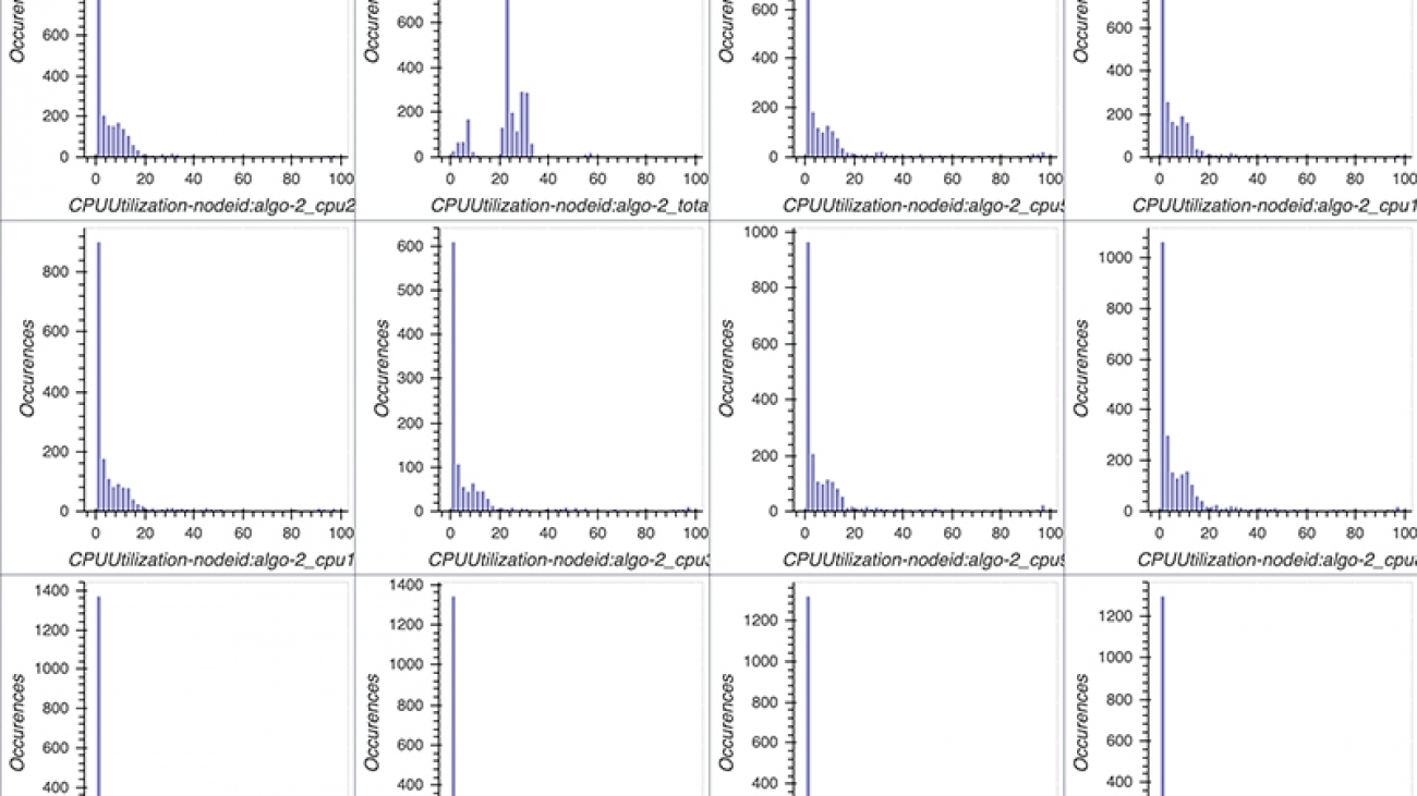
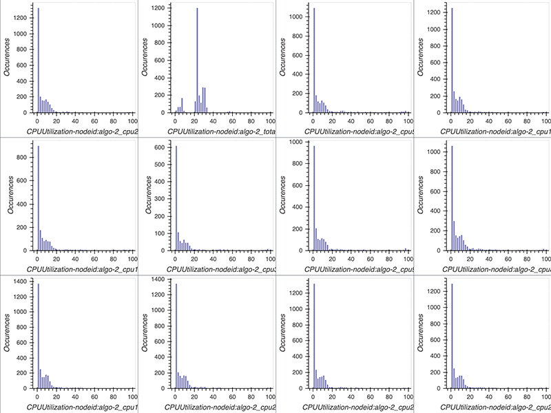
events = system_metrics_reader.get_events(0, last_timestamp)

Along with the notebook, the smdebug SDK contains several utility classes that can be used for visualizations. From the data collected, you can visualize the CPU and GPU utilization values as a histogram using the utility class MetricHistogram. MetricHistogram computes a histogram on GPU and CPU utilization values. Bins are between 0–100. Good system utilization means that the center of the distribution should be between 80–90. In case of multi-GPU training, if distributions of GPU utilization values aren’t similar, it indicates an issue with workload distribution.

The following code plots the histograms per metric. To only plot specific metrics, define the list select_dimensions and select_events. A dimension can be CPUUtilization, GPUUtilization, or GPUMemoryUtilization IOPS. If no event is specified, then for the CPU utilization, a histogram for each single core and total CPU usage is plotted.

from smdebug.profiler.analysis.notebook_utils.metrics_histogram import MetricsHistogram

system_metrics_reader.refresh_event_file_list()
metrics_histogram = MetricsHistogram(system_metrics_reader)

The following screenshot shows our histograms.

Similar to system metrics, let’s retrieve all the events emitted from the framework or algorithm metrics using the following code:

from smdebug.profiler.algorithm_metrics_reader import S3AlgorithmMetricsReader

framework_metrics_reader = S3AlgorithmMetricsReader(path)

events = []
while framework_metrics_reader.get_timestamp_of_latest_available_file() == 0 or len(events) == 0:
    framework_metrics_reader.refresh_event_file_list()
    last_timestamp = framework_metrics_reader.get_timestamp_of_latest_available_file()
    events = framework_metrics_reader.get_events(0, last_timestamp)

framework_metrics_reader.refresh_event_file_list()
last_timestamp = framework_metrics_reader.get_timestamp_of_latest_available_file()
events = framework_metrics_reader.get_events(0, last_timestamp)

We can inspect one of the recorded events to get the following:

print("Event name:", events[0].event_name, 
      "nStart time:", timestamp_to_utc(events[0].start_time/1000000000), 
      "nEnd time:", timestamp_to_utc(events[0].end_time/1000000000), 
      "nDuration:", events[0].duration, "nanosecond")

	Event name: Step:ModeKeys.TRAIN 
	Start time: 2020-12-04 22:44:14 
	End time: 2020-12-04 22:44:25 
	Duration: 10966842000 nanosecond

For more information about system and framework metrics, see documentation.

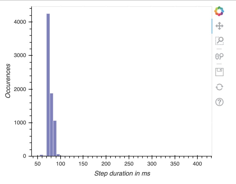
Next, we use the StepHistogram utility class to create a histogram of step duration values. Significant outliers in step durations are an indication of a bottleneck. It allows you to easily identify clusters of step duration values.

from smdebug.profiler.analysis.notebook_utils.step_histogram import StepHistogram
framework_metrics_reader.refresh_event_file_list()
step_histogram = StepHistogram(framework_metrics_reader)

The following screenshot shows our visualization.

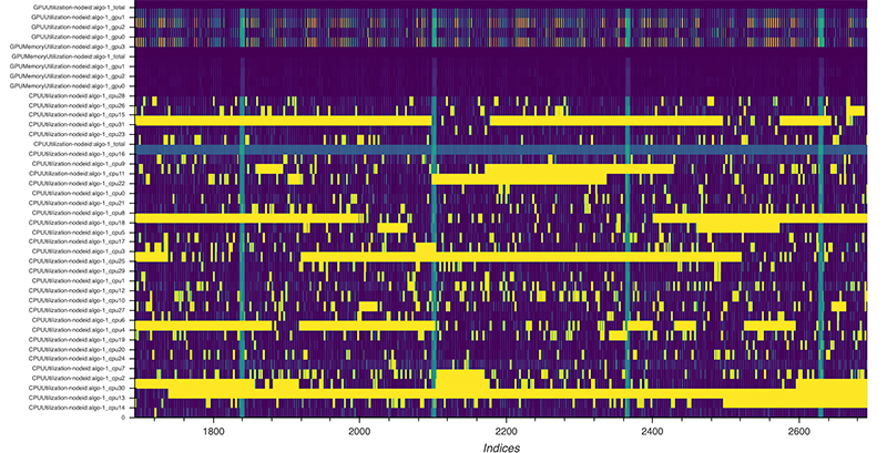
For an alternative view of CPU and GPU utilizations, the following code creates a heat map where each row corresponds to one metric (CPU core and GPU utilizations) and the x-axis is the duration of the training job. It allows you to more easily spot CPU bottlenecks, for example, if utilization on GPU is low but a utilization of one or more cores is high.

from smdebug.profiler.analysis.notebook_utils.heatmap import Heatmap

view_heatmap = Heatmap(
    system_metrics_reader,
    framework_metrics_reader,
    select_dimensions=["CPU", "GPU", "I/O"], # optional
    select_events=["total"],                 # optional
    plot_height=450
)

The following screenshot shows the heat map of a training job that has been using 4 GPUs and 32 CPU cores. The first few rows show the GPUs’ utilization, and the remaining rows show the utilization on CPU cores. Yellow indicates maximum utilization, and purple means that utilization was 0. GPUs have frequent stalled cycles where utilization drops to 0, whereas at the same time, utilization on CPU cores is at a maximum. This is a clear indication of a CPU bottleneck where GPUs are waiting for the data to arrive. Such a bottleneck can occur by a too compute-heavy preprocessing.

Accessing Debugger Insights in Studio

You can also use Studio to perform training with our existing notebook. Studio provides built-in visualizations to analyze profiling insights. Alternatively, you can move to next section in this post to directly analyze the profiler report generated.

If you trained in a SageMaker notebook instance, you can still find the Debugger insights for that training in Studio if the training happened in same Region.

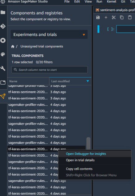
1. On the navigation pane, choose Components and registries.
2. Choose Experiments and trails.
3. Choose your training job (right-click).
4. Choose Debugger Insights.

For more information about setting up Studio, see Set up Amazon SageMaker.

Reviewing Debugger reports

After you have set up and run this notebook in Studio, you can access Debugger Insights.

1. On the navigation pane, choose Components and registries.
2. Choose Experiments and trails.
3. Choose your training job (right-click).
4. Choose View Debugger for insights.

A Debugger tab opens for this training job. For more information, see Debugger Insights.

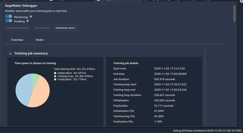
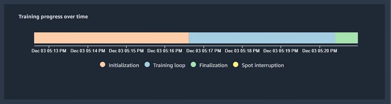
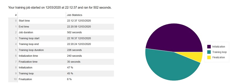
Training job summary

This section of the report shows details of the training job, such as the start time, end time, duration, and time spent in individual phases of the training. The pie chart visualization of these delays shows the time spent in initialization, training, and finalization phases relative to each other.

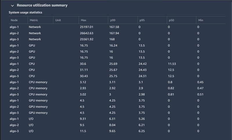
System usage statistics

This portion of the report gives detailed system usage statistics for both training instances involved in training, along with analysis and suggestions for improvements. The following text is an excerpt from the report, with key issues highlighted:

The 95th quantile of the total GPU utilization on node algo-1 is only 13%. The 95th quantile of the total CPU utilization is only 24%. Node algo-1 is under-utilized. You may want to consider switching to a smaller instance type. The 95th quantile of the total GPU utilization on node algo-2 is only 13%. The 95th quantile of the total CPU utilization is only 24%. Node algo-2 is under-utilized. You may want to consider switching to a smaller instance type. The 95th quantile of the total GPU utilization on node algo-3 is only 13%. The 95th quantile of the total CPU utilization is only 24%. Node algo-3 is under-utilized. You may want to consider switching to a smaller instance type.

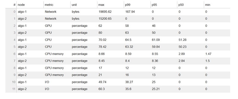
The following table shows usage statistics per worker node, such as total CPU and GPU utilization, total CPU, and memory footprint. The table also include total I/O wait time and total sent and received bytes. The table shows minimum and maximum values as well as p99, p90, and p50 percentiles.

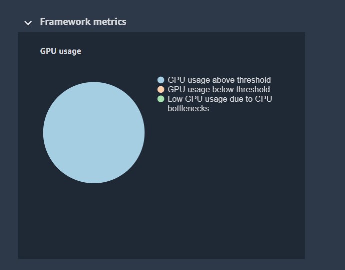
Framework metrics summary

In this section, the following pie charts show the breakdown of framework operations on CPUs and GPUs.

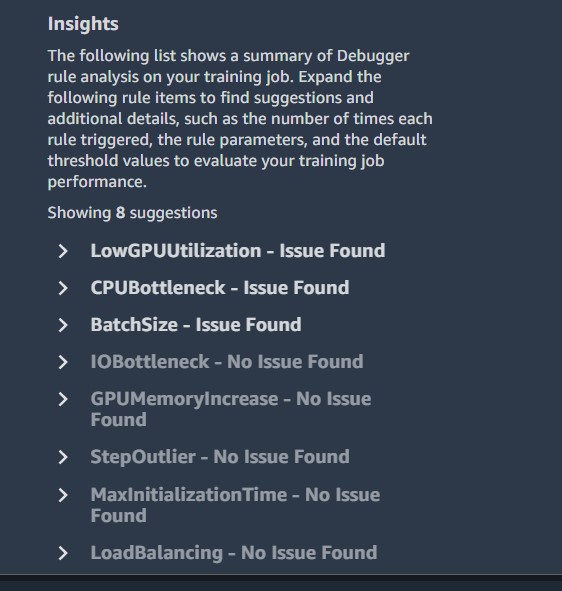
Insights

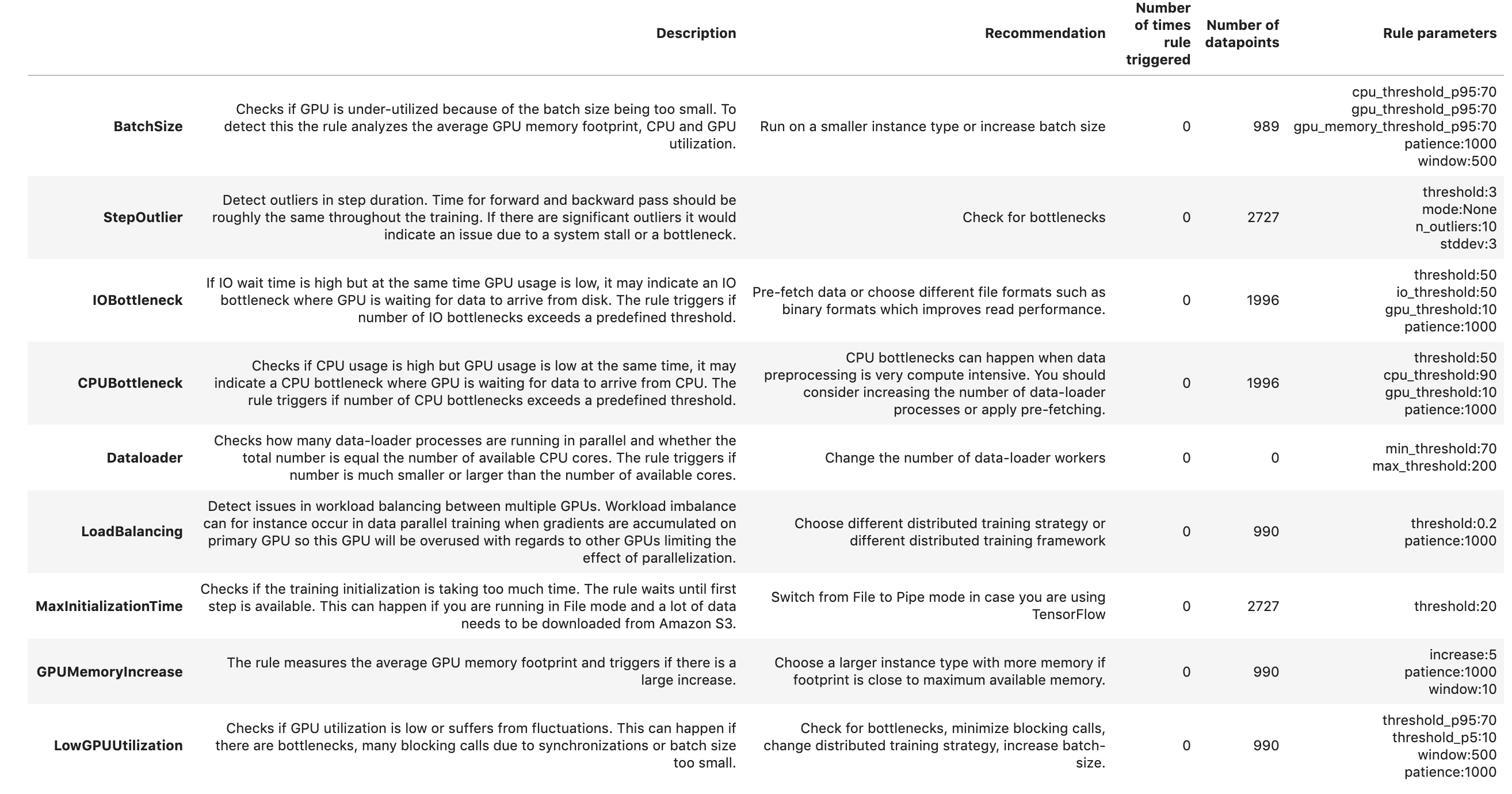
Insights provides suggestions and additional details, such as the number of times each rule triggered, the rule parameters, and the default threshold values to evaluate your training job performance. According to the insights for our TensorFlow training job, profiler rules were run for three out of the eight insights. The following screenshot shows the insights.

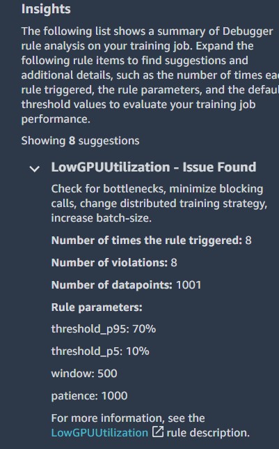
If you choose an insight, you can view the profiler recommendations.

By default, we are showing the overview report, but you could choose Nodes to show the dashboard.

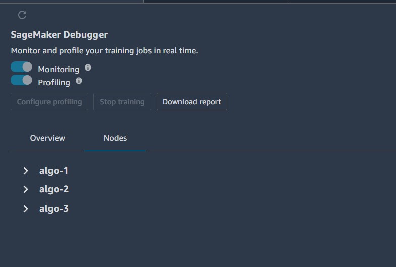
You can expand each algorithm to get deep dive information such as CPU utilization, network utilization, and system metrics per algorithm used during training.

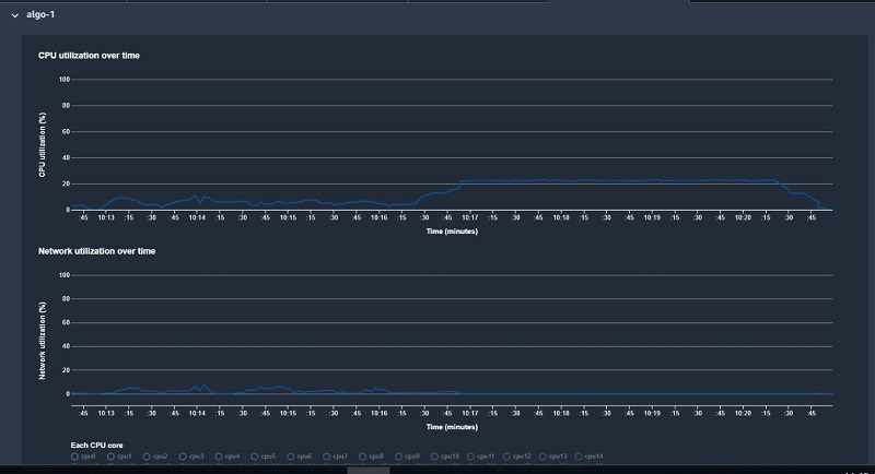
Furthermore, you can scroll down to analyze GPU memory utilization over time and system utilization over time for each algorithm.

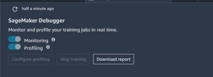
Analyzing the profiler report generated by Debugger

Download the profiler report by choosing Download report.

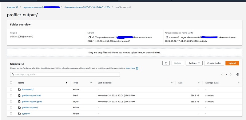
Alternatively, if you’re not using Studio, you can download your report directly from Amazon Simple Storage Service (Amazon S3) at s3://<your bucket> /tf-keras-sentiment-<job id>/profiler-output/.

Next, we review a few sections of the generated report. For additional details, see SageMaker Debugger report . You can also use the SMDebug client library for performing data analysis.

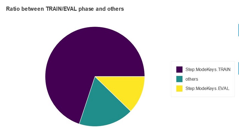
Framework metrics summary

In this section of the report, you see a pie chart that shows the time the training job spent in the training phase, validation phase, or “others.” “Others” represents the accumulated time between steps; that is, the time between when a step has finished but the next step hasn’t started. Ideally, most time should be spent in training steps.

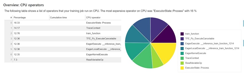
Identifying the most expensive CPU operator

This section provides information of the CPU operators in detail. The table shows the percentage of the time and the absolute cumulative time spent on the most frequently called CPU operators.

The following table shows a list of operators that your training job run on CPU. The most expensive operator on CPU was ExecutorState::Process with 16%.

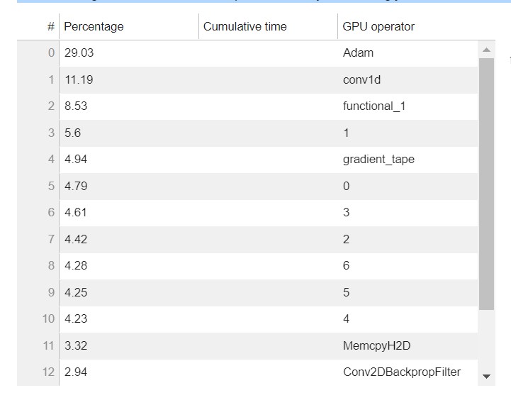
Identifying the most expensive GPU operator

This section provides information of the GPU operators in detail. The table shows the percentage of the time and the absolute cumulative time spent on the most frequently called GPU operators. 

The following table shows a list of operators that your training job ran on GPU. The most expensive operator on GPU was Adam with 29%.

Rules summary

In this section, Debugger aggregates all the rule evaluation results, analysis, rule descriptions, and suggestions. The following table shows a summary of the profiler rules that ran. The table is sorted by the rules that triggered most frequently. In the training job, this was the case for rule LowGPUUtilization. It processed 1,001 data points and was triggered 8 times.

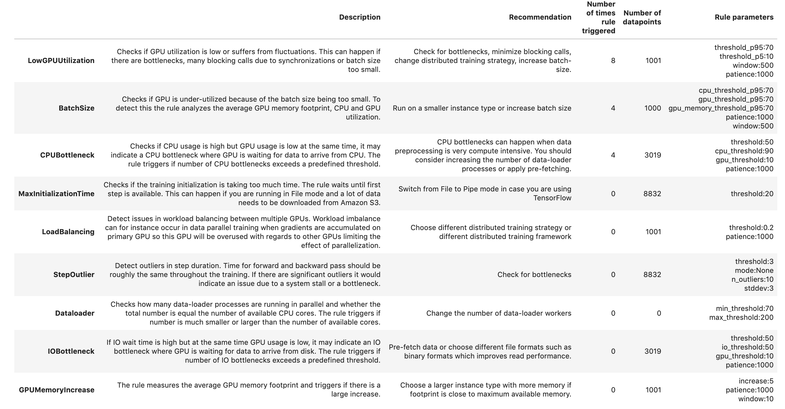
Because the rules were triggered for LowGPUUTilization, Batchsize, and CPUBottleneck, lets deep dive into each to understand the profiler recommendations for each.

LowGPUUtilization

The LowGPUUtilization rule checks for low and fluctuating GPU usage. If usage is consistently low, it might be caused by bottlenecks or if batch size or model is too small. If usage is heavily fluctuating, it can be caused by bottlenecks or blocking calls.

The rule computed the 95th and 5th quantile of GPU utilization on 500 continuous data points and found eight cases where p95 was above 70% and p5 was below 10%. If p95 is high and p5 is low, it indicates that the usage is highly fluctuating. If both values are very low, it means that the machine is under-utilized. During initialization, utilization is likely 0, so the rule skipped the first 1,000 data points. The rule analyzed 1,001 data points and was triggered eight times. Moreover it also provides the time when this rule was last triggered.

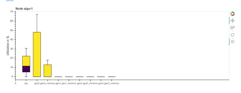
BatchSize

The BatchSize rule helps detect if GPU is under-utilized because of the batch size being too small. To detect this, the rule analyzes the GPU memory footprint and CPU and GPU utilization. The rule analyzed 1,000 data points and was triggered four times. Your training job is under-utilizing the instance. You may want to consider switching to a smaller instance type or increasing the batch size of your model training. Moreover it also provides the time when this rule was last triggered.

The following boxplot is a snapshot from this timestamp that shows for each node the total CPU utilization and the utilization and memory usage per GPU.

CPUBottleneck

The CPUBottleneck rule checks when CPU utilization was above cpu_threshold of 90% and GPU utilization was below gpu_threshold of 10%. During initialization, utilization is likely 0, so the rule skipped the first 1,000 data points. With this configuration, the rule found 2,129 CPU bottlenecks, which is 70% of the total time. This is above the threshold of 50%. The rule analyzed 3,019 data points and was triggered four times.

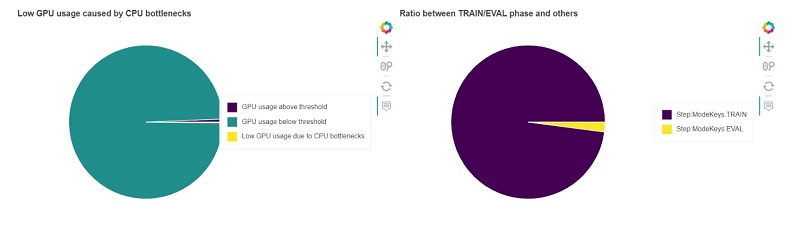
The following chart (left) shows how many data points were below the gpu_threshold of 10% and how many of those data points were likely caused by a CPU bottleneck. The rule found 3,000 out of 3,019 data points that had a GPU utilization below 10%. Out of those data points, 70.52% were likely caused by CPU bottlenecks. The second chart (right) shows whether CPU bottlenecks mainly happened during the train or validation phase.

Analyzing and implementing recommendations from the profiler report

Let’s now analyze and implement the profiling recommendations for our training job to improve resource utilization and make our training efficient. First let’s review the configuration of our training job and check the three rules that were triggered by Debugger during the training run.

The following table summarizes the training job configuration.

The following table summarizes the Debugger profiling recommendations.

Based on the recommendation to consider switching to a smaller instance type and to increase the batch size, we change the training configuration settings and rerun the training. In the notebook, the training instances are changed from p3.8xlarge to p3.2xlarge instances, the number of instances is reduced to two, and only one process per host for MPI is configured to increase the number of data loaders. The batch size is also changed in parallel to 512.

The following table summarizes the revised training job configuration. 

After running the second training job with the new settings, a new report is generated, but with no rules triggered, indicating all the issues identified in the earlier run were resolved. Now let’s compare the report analysis from the two training jobs and understand the impact of the configuration changes made.

The training job summary shows that the training time was almost similar, with 502 seconds in the revised run compared to 503 seconds in the first run. The amount of time spent in the training loop for both jobs was also comparable at 45%.

Examining the system usage statistics shows that both CPU and GPU utilization of the two training instances increased when compared to the original run. For the first training run, GPU utilization was constant at 13.5% across the three instances for the 95th quantile of GPU utilization, and the CPU utilization was constant at 24.4% across the three instances for the 95th quantile of CPU utilization. For the second training run, GPU utilization increased to 46% for the 95th quantile, and the CPU utilization increased to 61% for the 95th quantile.

Although no rules were triggered during this run, there is still room for improvement in resource utilization.

The following screenshot shows the rules summary for our revised training run.

You can continue to tune your training job, change the training parameters, rerun the training, and compare the results against previous training runs. Repeat this process to fine-tune your training strategy and training resources to achieve the optimal combination of training cost and training performance according to your business needs.

Optimizing costs

The following table shows a cost comparison of the two training runs.

Considering the cost of the training instances in a specific Region at the time of the this writing, for example us-west-2, training with three ml.p3.8xlarge instances for 503 seconds costs $6.16, and training with two ml.p3.2xlarge for 502 seconds costs $1.07. That is 83% cost savings by simply implementing the profiler recommendation to reduce the instance type.

Conclusion

The profiling feature of SageMaker Debugger is a powerful tool to gain visibility into ML training jobs. In this post, we provided insight into training resource utilization to identify bottlenecks, analyze the various phases of training, and identify expensive framework functions. We also showed how to analyze and implement profiler recommendations. We applied profiler recommendations to a TensorFlow Horovod distributed training for a sentiment analysis model and achieved resource utilization improvement up to 60% and cost savings of 83%. Debugger provides profiling capabilities for all leading deep learning frameworks, including TensorFlow, PyTorch, and Keras.

Give Debugger profiling a try and leave your feedback in the comments. For additional information on SageMaker Debugger, check out the announcement post linked below.

• New – Profile Your Machine Learning Training Jobs With Amazon SageMaker Debugger

About the Authors

Mona Mona is an AI/ML Specialist Solutions Architect based out of Arlington, VA. She works with the World Wide Public Sector team and helps customers adopt machine learning on a large scale. Prior to joining Amazon, she worked as an IT Consultant and completed her masters in Computer Information Systems from Georgia State University, with a focus in big data analytics. She is passionate about NLP and ML explainability in AI/ML.

Prem Ranga is an Enterprise Solutions Architect based out of Houston, Texas. He is part of the Machine Learning Technical Field Community and loves working with customers on their ML and AI journey. Prem is passionate about robotics, is an Autonomous Vehicles researcher, and also built the Alexa-controlled Beer Pours in Houston and other locations.

Sireesha Muppala is an AI/ML Specialist Solutions Architect at AWS, providing guidance to customers on architecting and implementing machine learning solutions at scale. She received her Ph.D. in Computer Science from the University of Colorado, Colorado Springs. In her spare time, Sireesha loves to run and hike Colorado trails.

Read More

We’re excited to announce the Amazon Forecast Weather Index, which can increase your forecasting accuracy by automatically including local weather information in your demand forecasts with one click and at no extra cost. Weather conditions influence consumer demand patterns, product merchandizing decisions, staffing requirements, and energy consumption needs. However, acquiring, cleaning, and effectively using live weather information for demand forecasting is challenging and requires ongoing maintenance. With this launch, you can now include 14-day weather forecasts for US and Europe locations with one click to your demand forecasts.

The Amazon Forecast Weather Index combines multiple weather metrics from historical weather events and current forecasts at a given location to increase your demand forecast model accuracy. Amazon Forecast uses machine learning (ML) to generate more accurate demand forecasts, without requiring any prior ML experience. Forecast brings the same technology used at Amazon.com to developers as a fully managed service, removing the need to manage resources or rebuild your systems.

Changes in local weather conditions can impact short-term demand for products and services at particular locations for many organizations in retail, hospitality, travel, entertainment, insurance, and energy domains. Although historical demand patterns show seasonal demand, advance planning for day-to-day variation is harder.

In retail inventory management use cases, day-to-day weather variation impacts foot traffic and product mix. Typical demand forecasting systems don’t take expected weather conditions into account, leading to stock-outs or excess inventory at some locations, resulting in the need to transfer inventory mid-week. For example, for retailers, knowing that a heat wave is expected, they may choose to over-stock air conditioners from distribution centers to specific store locations. Or they may choose to prepare different types of grab-and-go prepared food items depending on the weather conditions.

Outside of product demand, weather conditions also impact staffing needs. For example, restaurants can better balance staff dependent on dine-in vs. take-out orders, or businesses with warehouses can better predict the number of workers that may come into work because of disrupted transportation. Although store managers may be able to make one-off stocking decisions based on weather conditions using their intuition and judgment, making buying, inventory placement, and workforce management decisions at scale becomes more challenging.

Day-to-day weather variation also impacts hyper-local on-demand services that rely on efficient matching of supply and demand at scale. A looming storm can lead to high demand for local ride hailing or food delivery services, while also impacting the number of drivers available. Having the information of upcoming weather changes enables you to better meet customer demand. Programmatically applying local weather information at scale can help you preemptively match supply and demand.

Predicting future weather conditions is common, and although it’s possible to use these predictions to more accurately forecast demand for products and services, it may be a struggle to do so in practice. Acquiring your own historical weather data and weather forecasts is expensive, and requires constant data collation, aggregation, and cleaning. Additionally, without weather domain expertise, transforming raw weather metrics into predictive data is challenging.

With today’s launch, you can account for local day-to-day weather changes to better predict demand, with only one click and at no additional cost, using Forecast. When you use the Weather Index, Forecast trains a model with historical weather information for the locations of your operations and uses the latest 14-day weather forecasts on items that are influenced by day-to-day variations to create more accurate demand forecasts.

Tom Summerfield is the Director of Retail at Peak.AI, an accessible AI system that harnesses the power of data to assist—not displace—humans to improve business efficiency and productivity. Summerfield says, “At Peak, we work with retail, CPG, and manufacturing customers who all know that weather plays a strong role in dictating consumer buying habits. Variation in weather ultimately impacts their product demand and product basket mix. Our customers frequently ask us to include weather in their demand forecasts. With Amazon Forecast adding a weather feature, we are now able to seamlessly integrate these insights and improve the accuracy of our demand planning models.”

The Weather Index is currently optimized for in-store retail demand planning and local on-demand services, but may still add value to scenarios where weather impacts demand such as power and utilities. As of this writing, the Weather Index is only available for US and Europe Regions. Other Regions will become available soon. For more information about latitude-longitude bounding boxes and US zip codes supported, see Weather Index.

Using the Weather Index for your forecasting use case

You can add local weather information to your model by adding the Weather Index during training. In this section, we walk through the steps to use the Weather Index on the Forecast console. For this post, we use the New York City Taxi dataset. To review the steps through the APIs, refer to the following notebook in our GitHub repo, where we have a cleaned version of the New York Taxi dataset ready to be used.

The New York Taxi dataset has 260 locations and is being used to predict the demand for taxis per location per hour for the next 7 days (168 hours).

1. On the Forecast console, create a dataset group.

2. Upload the historical demand dataset as the target time series. This dataset must include geolocation information for you to use the Weather Index.
3. Select Schema builder.
4. Choose your location format (for this post, the dataset includes latitude and longitude coordinates). 

Forecast also supports postal codes for US only.

5. For Dataset import details, select Select time zone.
6. Choose your time zone (for this post, we choose America/New York).

You can apply a single time zone to the entire dataset, or ask Forecast to derive a time zone from the geolocation of each item ID in the target time series dataset.

7. In the navigation pane, under your dataset, choose Predictors.
8. Choose Train predictor.

9. For Forecast horizon, choose 168.
10. For Forecast frequency, choose hour.
11. For Number of backtest windows, choose 3.
12. For Backtest window offset, choose 168.
13. For Forecast types, choose p50, p60, and p70.
14. For Algorithm, you can either select AutoML for Forecast to find the best algorithm for your dataset or select a specific algorithm. For this post, we select DeepAR+ with Hyperparameter optimization turned on for Forecast to optimize the model.
15. Under Built-in datasets, select Enable Weather Index to apply the Weather Index to your training model. For this post, we have also selected Enable Holidays for US, as we hypothesize that holidays will have an impact on the demand for Taxis.

If you’re following the notebook in our GitHub repo, we call this predictor nyctaxi_demo_weather_deepar. While training the model, Forecast uses the historical weather to apply the Weather Index to only those items that are impacted by weather to improve item level accuracy.

16. After your predictor is trained, choose your predictor on the Predictors page to view the details of the accuracy metrics.

17. On the predictor’s details page, you can review the model accuracy numbers and choose Export backtest results in the Predictor metrics

Forecast provides different model accuracy metrics for you to assess the strength of your forecasting models. We provide the weighted quantile loss (wQL) metric for each selected distribution point, also called quantiles, and weighted absolute percentage error (WAPE) and root mean square error (RMSE), calculated at the mean forecast. For each metric, a lower value indicates a smaller error and therefore a more accurate model. All these accuracy metrics are non-negative. Quantiles are specified when choosing your forecast type. For more information about how each metric is calculated and recommendations for the best use case for each metric, see Measuring forecast model accuracy to optimize your business objectives with Amazon Forecast.

18. For S3 predictor backtest export location, enter the details of your Amazon Simple Storage Service (Amazon S3) location for exporting the CSV files.

Exporting the backtest results downloads the forecasts from the backtesting for each item and the accuracy metrics for each item. This helps you measure the accuracy of forecasts for individual items, allowing you to better understand your forecasting model’s performance for the items that most impact your business. For more information about the benefits of exporting backtest results, see Amazon Forecast now supports accuracy measurements for individual items.

In the next section of this post, we use these backtest results to assess the accuracy improvements of enabling the Weather Index by comparing the accuracy of specific items between models where you have not enabled the Weather Index.

19. After you evaluate the model accuracy, you can start creating forecasts by choosing Forecasts in the navigation pane.
20. Choose Create a forecast.

To create these forecasts, Forecast automatically pulls in the weather forecasts for the next 14 days and applies the weather prediction to only those item IDs that are influenced by weather. In our example, we create forecasts for the next 7 days with hourly frequency.

Assessing the impact of the Weather Index

To assess the impact of adding weather information to your forecasting models, we can create another predictor with the same dataset and settings, but this time without enabling the Weather Index. If you’re following the notebook in our GitHub repo, we call this predictor nyctaxi_demo_baseline_deepar.

When creating this predictor, you should not select Hyperparameter optimization for DeepAR+, but rather use the winning training parameters from the hyperparameter optimization of DeepAR+ model of nyctaxi_demo_weather_deepar as the training parameters setting, for a fair comparison between the two models. You can find the winning training parameters in the predictor details page under the Predictor metrics section. For this post, these are as follows.

"context_length": "63",
"epochs": "500",
"learning_rate": "0.014138165570842774",
"learning_rate_decay": "0.5",
"likelihood": "student-t",
"max_learning_rate_decays": "0",
"num_averaged_models": "1",
"num_cells": "40",
"num_layers": "2",
"prediction_length": "168"

You can then go to the Predictors page to review the predictor metrics nyctaxi_demo_baseline_deepar.

The following screenshot shows the predictor details page for the nyctaxi_demo_baseline_deepar model that is trained without enabling the Weather Index. The predictor metrics for nyctaxi_demo_weather_deepar with weather enabled is shown above after the create predictor steps.

The following table summarizes the predictor metrics for the two models. Forecast provides the weighted quantile loss (wQL) metric for each quantile, and weighted absolute percentage error (WAPE) metric and root mean square error (RMSE) metric, calculated at the mean forecast. For each metric, a lower value indicates a smaller error and therefore a more accurate model. The model with the Weather Index is more accurate, with lower values for each metric.

You can now export the backtest results for both predictors to assess the forecasting accuracy at an item level. With the backtest results, you can also use a visualization tool like Amazon QuickSight to create graphs that help you visualize and compare the model accuracy of both the predictors by plotting the forecasts against actuals for items that are important for you. The following graph visualizes the comparison of the models with and without the Weather Index to the actual demand for a few items in the dataset at the 0.60 quantile.

For Feb 27, we have zoomed in to better assess the difference in accuracies at an hourly level.

Here we show the magnitude of error for each item id for the two models. Lower error values correspond to a more accurate model. Most items in the model with the Weather Index have errors below 0.05.

Tips and best practices

When using the Weather Index, consider the following best practices:

• Before using the Weather Index, define your use case and the forecasting challenge. Evaluate if your business problem will be impacted by day-to-day weather, because the Weather Index is only available for short-term use cases of 14-day forecasts. Weekly, monthly, and yearly frequencies aren’t supported, so use cases where you are forecasting for the next season don’t benefit from the Weather Index. Only daily, hourly and minute frequencies are acceptable to use the Weather Index.
• For experimentation, start by identifying the most important item IDs for your business that you want to improve your forecasting accuracy. Measure the accuracy of your existing forecasting methodology as a baseline and compare that to the accuracy of those items with Forecast.
• Incrementally add the Weather Index, related time series, or item metadata to train your model to assess whether additional information improves accuracy. Different combinations of related time series, item metadata and built-in datasets can give you different results.
• To assess the impact of the Weather Index, first train a model with only your target time series, and then create another model with the Weather Index enabled. We recommend to use the same predictor settings for this comparison, because different hyperparameters and combinations of related time series can give you different results.
• You may see an increase in training costs when using the Weather Index, because the index is applied and optimized for only those items that are impacted by day-to-day weather variation. However, there is no extra cost to access the weather information or use the Weather Index for creating forecasts. The cost for training continues to be $0.24 per training hour and $0.60 per 1,000 forecasts.
• Experiment with multiple distribution points to optimize your forecast model to balance the costs associated with under-forecasting and over-forecasting. Choose a higher quantile if you want to over-forecast to meet demand.
• If you’re comparing different models, use the weighted quantile loss metric at the same quantile for comparison. The lower the value, the more accurate the forecasting model.
• Forecast allows you to select up to five backtest windows. Forecast uses backtesting to tune predictors and produce accuracy metrics. To perform backtesting, Forecast automatically splits your time series datasets into two sets: training and testing. The training set is used to train your model, and the testing set to evaluate the model’s predictive accuracy. We recommend choosing more than one backtest window to minimize selection bias that may make one window more or less accurate by chance. Assessing the overall model accuracy from multiple backtest windows provides a better measure of the strength of the model.

Conclusion

With the Amazon Forecast Weather Index, you can now automatically include local weather information to your demand forecasts with one click and at no extra cost. The Weather Index combines multiple weather metrics from historical weather events and current forecasts at a given location to increase your demand forecast model accuracy. To get started with this capability, see Weather Index and go through the notebook in our GitHub repo that walks you through how to use the Forecast APIs to enable the Weather Index. You can use this capability in all Regions where Forecast is publicly available. For more information about Region availability, see AWS Regional Services.

About the Authors

Namita Das is a Sr. Product Manager for Amazon Forecast. Her current focus is to democratize machine learning by building no-code/low-code ML services. On the side, she frequently advises startups and is raising a puppy named Imli.

Gunjan Garg is a Sr. Software Development Engineer in the AWS Vertical AI team. In her current role at Amazon Forecast, she focuses on engineering problems and enjoys building scalable systems that provide the most value to end-users. In her free time, she enjoys playing Sudoku and Minesweeper.

Christy Bergman is working as an AI/ML Specialist Solutions Architect at AWS. Her work involves helping AWS customers be successful using AI/ML services to solve real-world business problems. Prior to joining AWS, Christy worked as a data scientist in banking and software industries. In her spare time, she enjoys hiking and bird watching.

Read More