Monthly Archives: December 2020

Businesses are increasingly using machine learning (ML) to make near-real time decisions, such as placing an ad, assigning a driver, recommending a product, or even dynamically pricing products and services. ML models make predictions given a set of input data known as features, and data scientists easily spend more than 60% of their time designing and building these features. Furthermore, highly accurate predictions depend on timely access to feature values that change quickly over time, adding even more complexity to the job of building a highly available and accurate solution. For example, a model for a ride sharing app can choose the best price for a ri­de from the airport, but only if it knows the number of ride requests received in the past 10 minutes and the number of passengers projected to land in the next 10 minutes. A routing model in a call center app can pick the best available agent for an incoming call, but it is only effective if it knows the customer’s latest web session clicks.

Although the business value of near real time ML predictions is enormous, the architecture required to deliver them reliably, securely, and with good performance is complicated. Solutions need high-throughput updates and low latency retrieval of the most recent feature values in milliseconds, something most data scientists are not prepared to deliver. As a result, some enterprises have spent millions of dollars inventing their own proprietary infrastructure for feature management. Other firms have limited their ML applications to simpler patterns like batch scoring until ML vendors provide more comprehensive off-the-shelf solutions for online feature stores.

To address these challenges, Amazon SageMaker Feature Store provides a fully managed central repository for ML features, making it easy to securely store and retrieve features, without having to build and maintain your own infrastructure. Amazon SageMaker Feature Store lets you define groups of features, use batch ingestion and streaming ingestion, retrieve the latest feature values with single-digit millisecond latency for highly accurate online predictions, and extract point-in-time correct datasets for training. Instead of building and maintaining these infrastructure capabilities, you get a fully managed service that scales as your data grows, enables sharing features across teams, and lets your data scientists focus on building great ML models aimed at game-changing business use cases. Teams can now deliver robust features once, and reuse them many times in a variety of models that may be built by different teams.

This post walks through a complete example of how you can couple streaming feature engineering with Amazon SageMaker Feature Store to make ML-backed decisions in near-real time. We show a credit card fraud detection use case that updates aggregate features from a live stream of transactions and uses low-latency feature retrievals to help detect fraudulent transactions. Try it out for yourself by visiting our code repo.

Credit card fraud use case

Stolen credit card numbers can be bought in bulk on the dark web from previous leaks or hacks of organizations that store this sensitive data. Fraudsters buy these card lists and attempt to make as many transactions as possible with the stolen numbers until the card is blocked. These fraud attacks typically happen in a short time frame, and this can be easily spotted in historical transactions because the velocity of transactions during the attack differs significantly from the cardholder’s usual spending pattern.

The following table shows a sequence of transactions from one credit card where the cardholder first has a genuine spending pattern and then experiences a fraud attack starting on November 4^th.

For this post, we train an ML model to spot this kind of behavior by engineering features that describe an individual card’s spending pattern, such as the number of transactions or the average transaction amount from that card in a certain time window. This model protects cardholders from fraud at the point of sale by detecting and blocking suspicious transactions before the payment can complete. The model makes predictions in a low-latency, real-time context and relies on receiving up-to-the-minute feature calculations, so it can respond to an ongoing fraud attack. In a real-world scenario, features related to cardholder spending patterns would only form part of the model’s feature set, and we can include information about the merchant, the cardholder, the device used to make the payment, and any other data that may be relevant to detecting fraud.

Because our use case relies on profiling an individual card’s spending patterns, it’s crucial that we can identify credit cards in a transaction stream. Most publicly available fraud detection datasets don’t provide this information, so we use the Python Faker library to generate a set of transactions covering a 5-month period. This dataset contains 5.4 million transactions spread across 10,000 unique (and fake) credit card numbers and is intentionally imbalanced to match the reality of credit card fraud (only 0.25% of the transactions are fraudulent). We vary the number of transactions per day per card, as well as the transaction amounts. See our code repo for more detail.

Overview of the solution

We want our fraud detection model to classify credit card transactions by noticing a burst of recent transactions that differs significantly from the cardholder’s usual spending pattern. Sounds simple enough, but how do we build it?

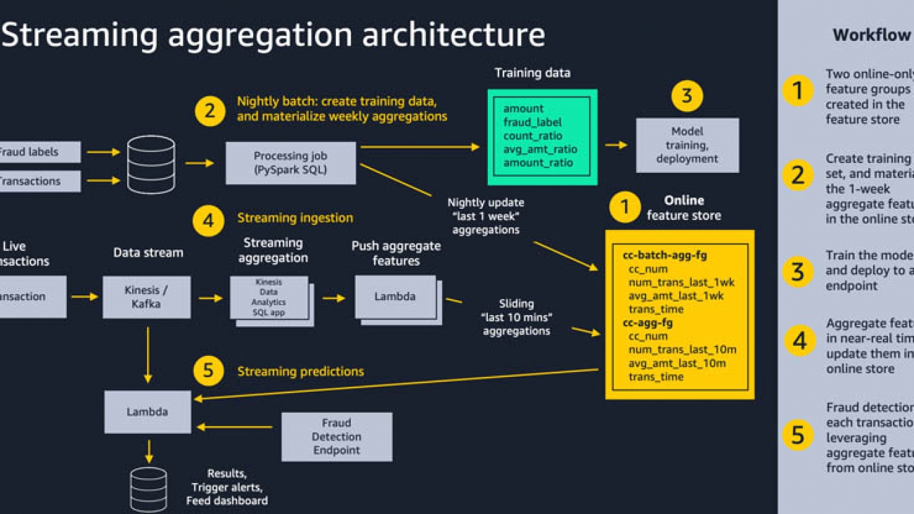
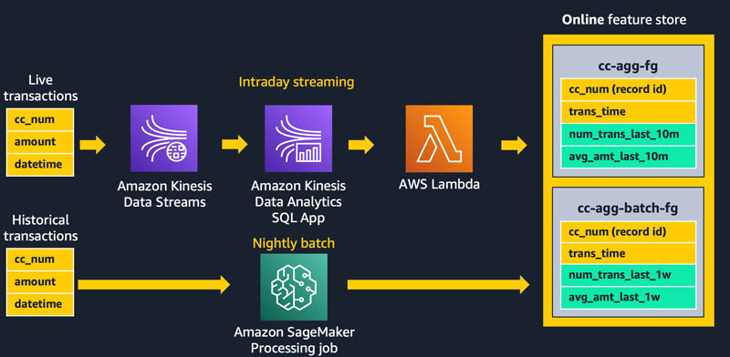
The following diagram shows our overall solution architecture. We feel that this same pattern will work well for a variety of streaming aggregation use cases. At a high level, the pattern involves the following five pieces. We dive into more detail on these in subsequent sections:

1. Feature store – We use Amazon SageMaker Feature Store to provide a repository of features with high-throughput writes and secure low-latency reads, using feature values that are organized into multiple feature groups.
2. Batch ingestion – Batch ingestion takes labeled historical credit card transactions and creates the aggregate features and ratios needed for training the fraud detection model. We use an Amazon SageMaker Processing job and the built-in Spark container to calculate aggregate weekly counts and transaction amount averages and ingest them into the feature store for use in online inference.
3. Model training and deployment – This aspect of our solution is straightforward. We use Amazon SageMaker to train a model using the built-in XGBoost algorithm on aggregated features created from historical transactions. The model is deployed to a SageMaker endpoint, where it handles fraud detection requests on live transactions.
4. Streaming ingestion – An Amazon Kinesis Data Analytics application calculates aggregated features from a transaction stream, and an AWS Lambda function updates the online feature store.
5. Streaming predictions – Lastly, we make fraud predictions on a stream of transactions, using AWS Lambda to pull aggregate features from the online feature store. We use the latest feature data to calculate transaction ratios and then call the fraud detection endpoint.

Feature store

ML models rely on well-engineered features coming from a variety of data sources, with transformations as simple as calculations, or as complicated as a multi-step pipeline that takes hours of compute time and complex coding. Amazon SageMaker Feature Store enables the reuse of these features across teams and models which improves data scientist productivity, speeds time to market, and ensures consistency of model input.

Each feature inside SageMaker Feature Store is organized into a logical grouping called a feature group. You decide which feature groups you need for your models. Each one can have dozens, hundreds, or even thousands of features. Feature groups are managed and scaled independently, but they’re all available for search and discovery across teams of data scientists responsible for many independent ML models and use cases.

ML models often require features from multiple feature groups. A key aspect of a feature group is how often its feature values need to be updated or materialized for downstream training or inference. You refresh some features hourly, nightly, or weekly, and a subset of features must be streamed to the feature store in near-real time. Streaming all feature updates would lead to unnecessary complexity, and could even lower the quality of data distributions by not giving you the chance to remove outliers.

In our use case, we create a feature group called cc-agg-batch-fg for aggregated credit card features updated in batch, and one called cc-agg-fg for streaming features. The batch feature group is updated nightly, and provides aggregate features looking back over a one-week time window. Recalculating one-week aggregations on streaming transactions does not offer meaningful signals, and would be a waste of resources.

Conversely, our cc-agg-fg feature group must be updated in a streaming fashion, because it offers the latest transaction counts and average transaction amounts looking back over a 10-minute time window. Without streaming aggregation, we could not spot the typical fraud attack pattern of a rapid sequence of purchases.

By isolating features that are recalculated nightly, we can improve ingestion throughput for our streaming features. Separation lets us optimize the ingestion for each group independently. When designing for your use cases, keep in mind that models requiring features from a large number of feature groups may want to make multiple retrievals from the feature store in parallel to avoid adding excessive latency to a real time prediction workflow.

The feature groups for our use case are seen in the following diagram.

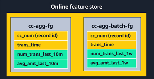
Each feature group must have one feature used as a record identifier (for this post, the credit card number). The record identifier acts as a primary key for the feature group, enabling fast lookups as well as joins across feature groups. An event time feature is also required, which enables the feature store to track the history of feature values over time. This becomes important when looking back at the state of features at a specific point in time.

In each feature group, we track the number of transactions per unique credit card and its average transaction amount. The only difference between our two groups is the time window used for aggregation. We use a 10-minute window for streaming aggregation, and a 1-week window for batch aggregation.

With Amazon SageMaker Feature Store, you have the flexibility to create feature groups that are offline only, online only, or both online and offline. An online store provides high-throughput writes and low-latency retrievals of feature values, ideal for online inference. An offline store is provided using Amazon S3, giving firms a highly scalable repository, with a full history of feature values, partitioned by feature group. The offline store is ideal for training and batch scoring use cases.

When you enable a feature group to provide both online and offline stores, SageMaker automatically synchronizes feature values to an offline store, continuously appending the latest values to give you a full history of values over time. Another benefit of feature groups that are both online and offline is to help avoid the problem of training and inference skew. SageMaker lets you feed both training and inference with the same transformed feature values, ensuring consistency to drive more accurate predictions. The focus in our post is to demonstrate online feature streaming, so we implemented online-only feature groups.

Batch ingestion

To materialize our batch features, we create a feature pipeline that is run as an Amazon SageMaker Processing job that is executed nightly. The job has two responsibilities: producing the dataset for training our model, and populating the batch feature group with the most up-to-date values for aggregate 1-week features, as shown in the following diagram:

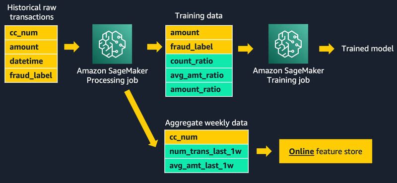
Each historical transaction used in the training set is enriched with aggregated features for the specific credit card involved in the transaction. We look back over two separate sliding time windows: 1 week back, and the preceding 10 minutes. The actual features used to train the model include the following ratios of these aggregated values:

• amt_ratio1 = avg_amt_last_10m / avg_amt_last_1w
• amt_ratio2 = transaction_amount / avg_amt_last_1w
• count_ratio = num_trans_last_10m / num_trans_last_1w

For example, the third ratio is the transaction count from the prior 10 minutes divided by the transaction count from the last week. Our ML model can learn patterns of normal activity versus fraudulent activity from these ratios, rather than relying on raw counts and transaction amounts. Spending patterns on different cards vary greatly, so normalized ratios provide a better signal to the model than the aggregated amounts themselves.

You may be wondering why our batch job is computing features with a 10-minute lookback. Isn’t that only relevant for online inference? We need the 10-minute window on historical transactions to create an accurate training dataset. This is critical for ensuring consistency with the 10-minute streaming window that will be used in near real time to support online inference.

The resulting training dataset from the processing job can be saved directly as a CSV for model training, or it can be bulk ingested into an offline feature group that can be used for other models and by other data science teams to address a wide variety of other use cases. For example, we can create and populate a feature group called cc-transactions-fg. Our training job can then pull a specific training dataset based on the needs for our specific model, selecting specific date ranges and a subset of features of interest. This approach enables multiple teams to reuse feature groups and maintain fewer feature pipelines, leading to significant cost savings and productivity improvements over time. This example notebook demonstrates the pattern of using SageMaker Feature Store as a central repository that data scientists can extract training datasets from.

In addition to creating a training dataset, we use the PutRecord API to put the 1-week feature aggregations into the online feature store nightly. The following code demonstrates putting a record into an online feature group given specific feature values, including a record identifier and an event time:

record = [{'FeatureName': 'cc_num', 
              'ValueAsString': str(cc_num)},
             {'FeatureName':'avg_amt_last_1w', 
              'ValueAsString': str(avg_amt_last_1w)},
             {'FeatureName':'num_trans_last_1w', 
              'ValueAsString': str(num_trans_last_1w)}]
event_time_feature = {
                 'FeatureName': 'trans_time',
                 'ValueAsString': str(int(round(time.time())))}
record.append(event_time_feature)
response = feature_store_client.put_record(
    FeatureGroupName=’cc-agg-batch-fg’, Record=record)

ML engineers often build a separate version of feature engineering code for online features based on the original code written by data scientists for model training. This can deliver the desired performance, but is an extra development step and introduces more chance for training and inference skew. In our use case, we show how using SQL for aggregations can enable a data scientist to provide the same code for both batch and streaming.

Streaming ingestion

Amazon SageMaker Feature Store delivers single-digit millisecond retrieval of pre-calculated features, and it can also play an effective role in solutions requiring streaming ingestion. Our use case demonstrates both. Weekly lookback is handled as a pre-calculated feature group, materialized nightly as shown earlier. Now let’s dive into how we calculate features aggregated on the fly over a 10-minute window and ingest them into the feature store for later online inference.

You can perform streaming ingestion by tapping into an Apache Kafka topic or an Amazon Kinesis Data Stream, applying feature transformation and aggregation, and pushing the result to the feature store. For teams comfortable with Java, Apache Flink is a popular framework for streaming aggregation. However, for data scientists with limited Java skills, SQL is a much more accessible option.

In our use case, we listen to a Kinesis data stream of credit card transactions, and use a simple Kinesis Data Analytics SQL application to create aggregate features. An AWS Lambda function ingests those features into the feature store for subsequent use at inference time. Establishing the SQL app is straightforward. You choose a source stream, define a SQL query, and identify a destination (for our use case, a Lambda function).

To produce aggregate counts and average amounts looking back over a 10-minute window, we use the following SQL query on the input stream:

SELECT STREAM "cc_num",
               COUNT(*) OVER LAST_10_MINUTES,
               AVG("amount") OVER LAST_10_MINUTES
FROM transactions WINDOW LAST_10_MINUTES AS (PARTITION BY "cc_num" RANGE INTERVAL '10' MINUTE PRECEDING)

In this example, notice that the final row has a count of four transactions in the last 10 minutes from the credit card ending with 1248, and a corresponding average transaction amount of $200.00. The SQL query is consistent with the one used to drive creation of our training dataset, helping to avoid training and inference skew.

As transactions stream into the SQL app, the app sends the aggregate results to our Lambda function, as shown in the following diagram. The Lambda function takes these features and populates the cc-agg-fg feature group.

Updating feature values in the feature store from Lambda is done using a simple call to the PutRecord API. The following is the core piece of Python code for storing the aggregate features:

record = [{'FeatureName': 'cc_num', 
           'ValueAsString': str(cc_num)},
          {'FeatureName':'avg_amt_last_10m', 
           'ValueAsString': str(avg_amt_last_10m)},
          {'FeatureName':'num_trans_last_10m', 
           'ValueAsString': str(num_trans_last_10m)},
          {'FeatureName': 'evt_time', 
           'ValueAsString': str(int(round(time.time())))}]
featurestore_runtime.put_record(FeatureGroupName='cc-agg-fg', 
                                Record=record)

We prepare the record as a list of named value pairs, including the current time as the event time. The SageMaker Feature Store API ensures that this new record follows the schema that we identified when we created the feature group. If a record for this primary key already existed, it is now overwritten in the online store.

Streaming predictions

Now that we have streaming ingestion keeping the feature store up to date with the latest feature values, let’s look at how we make fraud predictions.

We create a second Lambda function that uses a Kinesis data stream as a trigger. For each new transaction event, we retrieve batch and streaming features from SageMaker Feature Store, calculate ratios, and invoke the SageMaker model endpoint to make the prediction as shown in the following diagram.

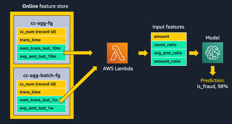
We use the following code to retrieve feature values on demand from the feature store before calling the SageMaker model endpoint:

featurestore_runtime =  
        boto3.client(service_name='sagemaker-featurestore-runtime')
response = featurestore_runtime.get_record(
		FeatureGroupName=feature_group_name, 
        RecordIdentifierValueAsString=record_identifier_value)

Finally, with the model input feature vector assembled, we call the model endpoint to predict if a specific credit card transaction is fraudulent:

sagemaker_runtime =  
    boto3.client(service_name='runtime.sagemaker')
request_body = ','.join(features)
response = sagemaker_runtime.invoke_endpoint(
    EndpointName=ENDPOINT_NAME,
    ContentType='text/csv',
    Body=request_body)
probability = json.loads(response['Body'].read().decode('utf-8'))

In the example above, the model came back with a probability of 98% that the specific transaction was fraudulent, and it was able to leverage near real-time aggregated input features, based on the most recent 10 minutes of transactions on that credit card.

Seeing it work end to end

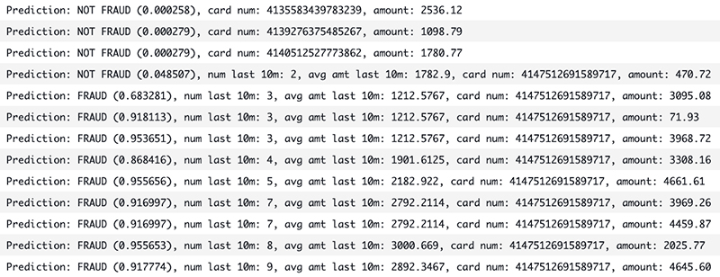
To demonstrate the full end-to-end workflow of our solution, we simply send credit card transactions into our Kinesis data stream. Our automated streaming feature aggregation takes over from there, maintaining a near real time view of transaction counts and amounts in SageMaker Feature Store, with a sliding 10-minute lookback window. These features are combined with the 1-week aggregate features that were already ingested to the feature store in batch, letting us make fraud predictions on each transaction.

We send a single transaction from three different credit cards. We then simulate a fraud attack on a fourth credit card by sending many back-to-back transactions in seconds. The output from our Lambda function is shown below. As expected, the first three one-off transactions are predicted as NOT FRAUD. Of the 10 fraudulent transactions, the first is predicted as NOT FRAUD, and the rest are all correctly identified as FRAUD. Notice how the aggregate features are kept current, helping drive more accurate predictions.

Conclusion

We have shown how Amazon SageMaker Feature Store can play a key role in the solution architecture for critical operational workflows that need streaming aggregation and low latency inference. With an enterprise-ready feature store in place, you can use both batch ingestion and streaming ingestion to feed feature groups, and access feature values on demand to perform online predictions for significant business value. ML features can now be shared at scale across many teams of data scientists and thousands of ML models, improving data consistency, model accuracy, and data scientist productivity. Amazon SageMaker Feature Store is available now, and you can try out this entire example. Let us know what you think.

About the Authors

Paul Hargis is an AI/ML Specialist, Solutions Architect at Amazon Web Services (AWS). Prior to this role, he was lead architect for Amazon Exports and Expansions helping amazon.com improve experience for international shoppers. Paul likes to help customers expand their machine learning initiatives to solve real-world problems. He is married and has one daughter who runs in Cross Country and Track teams in high school.

Megan Leoni is an AI/ML Specialist Solutions Architect for AWS helping customers across Europe, Middle East, and Africa design and implement ML Solutions. Prior to joining AWS, Megan worked as a data scientist building and deploying real time fraud detection models.

Mark Roy is a Principal Machine Learning Architect for AWS, helping AWS customers design and build AI/ML solutions. Mark’s work covers a wide range of ML use cases, with a primary interest in computer vision, deep learning, and scaling ML across the enterprise. He has helped companies in many industries, including Insurance, Financial Services, Media and Entertainment, Healthcare, Utilities, and Manufacturing. Mark holds 6 AWS certifications, including the ML Specialty Certification. Prior to joining AWS, Mark was an architect, developer, and technology leader for 25+ years, including 19 years in financial services.

Arunprasath Shankar is an Artificial Intelligence and Machine Learning (AI/ML) Specialist Solutions Architect with AWS, helping global customers scale their AI solutions effectively and efficiently in the cloud. In his spare time, Arun enjoys watching sci-fi movies and listening to classical music.

Read More

Note: At the AWS re:Invent Machine Learning Keynote we announced performance records for T5-3B and Mask-RCNN. This blog post includes updated numbers with additional optimizations since the keynote aired live on 12/8.

At re:Invent 2019, we demonstrated the fastest training times on the cloud for Mask R-CNN, a popular instance segmentation model, and BERT, a popular natural language processing (NLP) model. Over the past several months, we have worked in collaboration with NVIDIA to significantly improve the underlying infrastructure, network, machine learning (ML) framework, and model code to once again achieve the best training times for state-of-the-art models used by our customers. Today, we’re excited to share with you the fastest training times for Mask R-CNN on TensorFlow and PyTorch and T5-3B (NLP) on PyTorch, and dive deep into the technology stack, our optimizations, and how you can leverage these capabilities to train large models quickly with Amazon SageMaker.

Summary results

Our customers training deep neural network models in PyTorch and TensorFlow have asked for help with problems they face with training speed and model size. First, customers told us they wanted to train models faster without waiting days or weeks for results. Data scientists need to iterate daily to get ML applications to market faster. Second, customers told us they struggled to apply the latest research in NLP because these model architectures didn’t fit in a single NVIDIA GPU’s memory during training. Customers knew they could get higher accuracy from these larger models with billions of parameters. But there was no easy way to automatically and efficiently split a model across multiple NVIDIA GPUs.

To solve these problems, AWS released new SageMaker distributed training libraries, which provide the easiest and fastest way to train deep learning models. The SageMaker data parallelism library provides better scaling efficiency than Horovod or PyTorch’s Distributed Data Parallel (DDP), and its model parallelism library automatically splits large models across multiple GPUs. In this post, we describe how this underlying technology was used to achieve record training times for Mask R-CNN and T5-3B.

Mask R-CNN

Object detection algorithms form the backbone of many deep learning applications. Self-driving cars, security systems, and image processing all incorporate object detection. In particular, Mask R-CNN is ubiquitous in this field. Mask R-CNN takes in an image and then isolates and identifies objects within that image, providing both a bounding box and object mask. Since it was first proposed in 2017, training Mask R-CNN on the COCO dataset has become the standard benchmark for object detection models, and many of our customers use this as their baseline to build their own models.

One issue with Mask R-CNN is its complexity. The model incorporates multiple different neural networks performing different tasks. One network identifies candidate objects, while two others are responsible for identifying objects and generating masks. In addition, the model must perform operations like non-max suppression and sample selection, which can be difficult to optimize on the GPU. In the original 2017 paper, Mask R-CNN took 32 hours to train on 8 GPUs with the COCO data. Since then, training time has significantly improved. In 2019, we demonstrated the fastest training times in the cloud for Mask R-CNN—27 minutes with PyTorch and 28 minutes with TensorFlow. In 2020, we collaborated with NVIDIA to bring this down to 6:45 minutes on PyTorch and 6:12 minutes on TensorFlow. To our knowledge, this is the fastest time to train Mask R-CNN in the cloud and a 75% reduction from our record last year.

Mask-RCNN Technology stack and performance

Achieving these results required optimizations to the underlying hardware, networking, and software stack. We added GPU implementations of some operations that are central to training Mask R-CNN. We also added new data pipelining utilities to speed up pre-processing and avoid any degradation in GPU utilization. In collaboration with NVIDIA, we deployed a new optimizer, NovoGrad, to push the boundaries further on large batch training. All of these optimizations are available in SageMaker, the AWS Deep Learning Containers, and the AWS Deep Learning AMIs. The result is that our training times this year are more than twice as fast on a single-node workload, and more than three times as fast on a multi-node workload, as compared to 2019.

Next, we scaled this optimized single-node workload to a cluster of 64 p3dn.24xlarge instances, each with 8 NVIDIA V100 GPUs. Efficiently scaling to 512 V100 GPUs requires fully utilizing the available bandwidth and topology between Amazon Elastic Compute Cloud (Amazon EC2) instances. At SC20 this year, we demonstrated a reimagined parameter server at scale that was designed from scratch to use the AWS Elastic Fabric Adapter (EFA) and node-to-node communication between EC2 instances. This technology is available to developers as of today with the SageMaker data parallelism library, with native framework APIs for both TensorFlow and PyTorch.

Distributed training generally uses one of two distribution strategies: parameter servers or AllReduce. Although parameter servers can perform gradient reduction with less communication than AllReduce (2 hops vs. 2(n-1) hops, respectively) and can perform asynchronous parameter updates, parameter servers tend to suffer from uneven bandwidth allocation and network congestion. Both drawbacks become more apparent with larger clusters. As a result, AllReduce is more often used. However, AllReduce has its own drawbacks. In addition to the increased number of hops, AllReduce requires synchronous updates between nodes, meaning all training is impacted by a single straggler node.

We can use EFA to overcome network congestion by spreading communication evenly across multiple routes between nodes. In addition, SageMaker introduces a balanced fusion buffer, which collects gradients on each GPU and shards them evenly to each parameter server, ensuring a balanced workload across the entire cluster. The results show significantly improved scaling efficiency, and reduced training times on larger clusters. With SageMaker, along with new large batch optimizations, we can efficiently scale both TensorFlow and PyTorch to 512 A100 GPUs, while scaling almost linearly. With these new tools, we can train Mask R-CNN to convergence in just above 6 minutes on both frameworks, beating last year’s best time by more than 75%. The following charts show the improvement in scaling efficiency using SageMaker’s data parallelism library when training Mask-RCNN relative to DDP and Horovod.

T5-3B: Text-to-Text Transfer Transformer

We’ve seen rapid progress in NLP model accuracy in the past few years. In 2017, we saw the invention of the transformer layer, a novel way for models to identify the portion of the text to focus on. We then saw state-of-the-art models such as BERT, RoBERTa, ALBERT, and DistilBERT. Now we see researchers achieving record accuracy and zero- or few-shot learning with large models that have billions or hundreds of billions of parameters.

Empirical results from OpenAI show that optimal performance comes from scaling up in three dimensions: model size, dataset size, and training steps. Model size is the primary bottleneck, and for smaller models such as BERT, data parallelism alone has been sufficient. Yet scaling to extreme language model sizes has been prohibitively difficult for developers and researchers because models can no longer fit onto a single GPU’s memory, preventing any data parallelism from taking place.

T5 is 15 times larger than the original BERT model and achieved near-human performance on the SuperGLUE benchmark. In addition, sequence-to-sequence models can perform machine translation, text summarization, and open-domain question-answering. In collaboration with NVIDIA, who supplied the base technology for T5 pre-training and fine-tuning tasks [1], we trained T5-3B in 4.86 days on 2,048 A100 GPUs on 256 p4d.24xlarge instances. The technologies for automatic and efficient splitting of large models across multiple GPU devices are now available in SageMaker.

T5-3B Technology stack and performance

SageMaker splits the model into multiple partitions that each fit on a single GPU. The freed memory can then be used to scale to larger batch sizes, further increasing training throughput and speeding up convergence. SageMaker also implements pipelined execution that splits data into smaller micro-batches and interleaves execution to increase GPU utilization.

The following figure illustrates an example execution schedule for the interleaved pipeline over two GPUs. F0 represents the forward pass for micro-batch 0, and B1 represents the backward pass for micro-batch 1. “Update” represents the optimizer update of the parameters. The figure shows that GPU0 always prioritizes backward passes whenever possible (for instance, running B0 before F2), which allows for clearing the memory used for activations earlier.

To train T5-3B, SageMaker performed 8-way model parallel training combined with 256-way data parallel training. We further improved training time by using the new p4d.24xlarge instances, equipped with 8 NVIDIA A100 GPUs and supporting 400 Gbps network bandwidth. We reduced the training time to 4.86 days by efficiently scaling out to 256 instances. We used EFA to optimize network communication over large clusters. We achieved the best training performance by using SageMaker, 256 p4d.24xlarge instances, and EFA.

To evaluate model performance, we fine-tuned the pre-trained checkpoints on a downstream natural language inference task. We used the Multi-Genre Natural Language Inference (MNLI) corpus for fine-tuning. The corpus contains around 433,000 hypothesis/premise sentence pairs and covers a range of genres of spoken and written text with support for cross-genre evaluation. We obtained a score of 91.19 for in-genre (matched) and a score of 91.25 for cross-genre (mismatched) in only 4.86 days time to train.

Conclusion

With these new record-breaking training times, AWS continues to be the industry leader in cloud ML. These models are now available for everyone to use in AWS by leveraging the new SageMaker data parallelism and model parallelism libraries. You can get started with distributed training on SageMaker using the following examples. For further information, please feel free to reach out to Aditya Bindal directly at bindala@amazon.com.

Editor’s Note: All of the following contributors were essential to our ability to achieve this year’s results and to the writing of this post: Abhinav Sharma, Anurag Singh, Gautam Kumar, Harsh Patel, Lai Wei, Rahul Huilgol, Rejin Joy, Roshani Nagmote, Sami Kama, Sam Oshin, Qinggang Zhou, Yu Liu

About the Authors

Aditya Bindal is a Senior Product Manager for AWS Deep Learning. He works on products that make it easier for customers to train deep learning models on AWS. In his spare time, he enjoys spending time with his daughter, playing tennis, reading historical fiction, and traveling.

Ben Snyder is an applied scientist with AWS Deep Learning. His research interests include computer vision models, reinforcement learning, and distributed optimization. Outside of work, he enjoys cycling and backcountry camping.

Derya Cavdar is currently working as a software engineer at AWS AI in Palo Alto, CA. She received her PhD in Computer Engineering from Bogazici University, Istanbul, Turkey, in 2016. Her research interests are deep learning, distributed training optimization, large-scale machine learning systems, and performance modeling.

Jared Nielsen is an Applied Scientist with AWS Deep Learning. His research interests include natural language processing, reinforcement learning, and large-scale training optimizations. He is a passionate rock climber outside of work.

Khaled ElGalaind is the engineering manager for AWS Deep Engine Benchmarking, focusing on performance improvements for AWS machine learning customers. Khaled is passionate about democratizing deep learning. Outside of work, he enjoys volunteering with the Boy Scouts, BBQ, and hiking in Yosemite.

Brian Pickering is the VP of Sales & Business Development – Amazon Relationship at NVIDIA. He joined NVIDIA in 2016 to manage NVIDIA’s relationship with Amazon. Prior to NVIDIA, Brian was at F5 Networks, where he led their Cloud Sales and Cloud Partner Ecosystem. In 2012, while at AWS and responsible for leading the AWS Consulting Partner Ecosystem program and teams, CRN recognized Brian as one of the top 100 “People You Don’t Know But Should for Channel.” Prior to AWS, Brian lead various strategic business efforts, including winning the first non-MS OS OEM deal with Dell while at Red Hat.

Anish Mohan is a Machine Learning Architect at NVIDIA and the technical lead for ML/DL engagements with key NVIDIA customers in the greater Seattle region. Before NVIDIA, he was at Microsoft’s AI Division, working to develop and deploy AI/ML algorithms and solutions.

Read More

Amazon SageMaker Autopilot automatically trains and tunes the best machine learning (ML) models for classification or regression problems while allowing you to maintain full control and visibility. This not only allows data analysts, developers, and data scientists to train, tune, and deploy models with little to no code, but you can also review a generated notebook that outlines all the steps that Autopilot took to generate the model. In some cases, you might also want to customize pipelines generated by Autopilot with your own custom components.

This post shows you how to create and use models with Autopilot in a couple of clicks, then outlines how to adapt the SageMaker Autopilot generated code with your own feature selectors and custom transformers to add domain-specific features. We also use the dry run capability of Autopilot, in which Autopilot only generates code for data preprocessors, algorithms, and algorithm parameter settings. This can be done by simply choosing the option run a pilot to create a notebook with candidate definitions.

Customizing Autopilot

Customizing Autopilot models is, in most cases, not necessary. Autopilot creates high-quality models that can be deployed without the need for customization. Autopilot automatically performs exploratory analysis of your data and decides which features may produce the best results. As such, it presents a low barrier of entry to ML for a wide range of users, from data analysts to developers, wishing to add AI/ML capabilities to their project.

However, more advanced users can take advantage of Autopilot’s transparent approach to AutoML to dramatically reduce the undifferentiated heavy lifting prevalent in ML projects. For example, you may want Autopilot to use custom feature transformations that your company uses, or custom imputation techniques that work better in the context of your data. You can preprocess your data before bringing it to SageMaker Autopilot, but that would involve going outside Autopilot and maintaining a separate preprocessing pipeline. Alternatively, you can use Autopilot’s data processing pipeline to direct Autopilot to use your custom transformations and imputations. The advantage to this approach is that you can focus on data collection, and let Autopilot do the heavy lifting to apply your desired feature transformations and imputations, and then find and deploy the best model.

Preparing your data and Autopilot job

Let’s start by creating an Autopilot experiment using the Forest Cover Type dataset.

1. Download the dataset and upload it to Amazon Simple Storage Service (Amazon S3).

Make sure that you create your Amazon SageMaker Studio user in the same Region as the S3 bucket.

2. Open SageMaker Studio.
3. Create a job, providing the following information:
   1. Experiment name
   2. Training dataset location
   3. S3 bucket for saving Autopilot output data
   4. Type of ML problem

Your Autopilot job is now ready to run. Instead of running a complete experiment, we choose to let Autopilot generate a notebook with candidate definitions.

Inspecting the Autopilot-generated pipelines

SageMaker Autopilot automates the key tasks in an ML pipeline. It explores hundreds of models comprised of different features, algorithms, and hyperparameters to find the one that best fits your data. It also provides a leader board of 250 models so you can see how each model candidate performed and pick the best one to deploy. We explore this in more depth in the final section of this post.

When the experiment is complete, you can inspect your generated candidate pipelines. Candidate refers to the combination of data preprocessing steps and algorithm selection used to train the 250 models. The candidate generation notebook contains Python code that Autopilot used to generate these candidates.

1. Choose Open candidate generation notebook.
2. Open your notebook.
3. Choose Import to import the notebook into your workspace.
4. When prompted, choose Python 3 (Data Science) as the kernel.
5. Inside the notebook, run all the cells in the SageMaker Setup

This copies the data preparation code that Autopilot generated into your workspace.

In your root SageMaker Studio directory, you should now see a folder with the name of your Autopilot experiment. The folder’s name should be <Your Experiment Name>–artifacts. That directory contains two sub-directories: generated_module and sagemaker_automl. The generated_module directory contains the data processing artifacts that Autopilot generated.

So far, the Autopilot job has analyzed the dataset and generated ML candidate pipelines that contain a set of feature transformers and an ML algorithm. Navigate down the generated_module folder to the candidate_data_processors directory, which contains 12 files:

• dpp0.py–dpp9.py – Data processing candidates that Autopilot generated
• trainer.py – Script that runs the data processing candidates
• sagemaker_serve.py – Script for running the preprocessing pipeline at inference time

If you examine any of the dpp*.py files, you can observe that Autopilot generated code that builds sckit-learn pipelines, which you can easily extend with your own transformations. You can do this by either modifying the existing dpp*.py files directly or extending the pipelines after they’re instantiated in the trainer.py file, in which you define a transformer that can be called inside existing dpp*.py files. The second approach is recommended because it’s more maintainable and allows you to extend all the proposed processing pipelines at once as opposed to modifying each one individually.

Using specific transformers

You may wish to call a specific transformer from sckit-learn or use one implemented in the open-source package sagemaker-scikit-learn-extension. The latter provides a number of scikit-learn-compatible estimators and transformers that you can use. For instance, it implements the Weight of Evidence (WoE) encoder, an often-used encoding for categorical features in the context of binary classification.

To use additional transformers, first extend the import statements in the trainer.py file. For our use case, we add the following code:

from sklearn.pipeline import FeatureUnion, Pipeline
from sklearn.ensemble import RandomForestClassifier
from sklearn.feature_selection import SelectFromModel
from sagemaker_sklearn_extension.preprocessing import RobustStandardScaler

If, upon modifying trainer.py, you encounter errors when running the notebook cell containing automl_interactive_runner.fit_data_transformers(...), you can get debugging information from Amazon CloudWatch under the log group /aws/sagemaker/TrainingJobs.

Implementing custom transformers

Going back to the forest cover type use case, we have features for the vertical and horizontal distance to hydrology. We want to extend this with an additional feature transform that calculates the straight line distance to hydrology. We can do this by adding an additional file into the candidate_data_processors directory where we define our custom transform. See the following code:

# additional_features.py
import numpy as np
from sklearn.base import BaseEstimator, TransformerMixin

class HydrologyDistance(BaseEstimator, TransformerMixin):

    def __init__(self, feature_index):
        self._feature_index = feature_index
      
    def fit(self, X, y = None):
        return self 
    
    def transform(self, X, y = None):
        X = X.copy().astype(np.float32)
        a, b = np.split(X[:, self._feature_index ], 2, axis=1)
        return np.hypot(a,b).reshape(-1,1)

Inside the trainer.py file, we then import the additional_features module and add our HydrologyDistance transformer as a parallel pipeline to the existing generated ones.

In addition to our additional feature transformer, we also add a feature selector to our pipeline to select only the features with the highest importance as determined by a RandomForestClassifier:

def update_feature_transformer(header, feature_transformer):
    """Customize the feature transformer. Default returns

    header: sagemaker_sklearn_extension.externals.Header
        Object of class Header, used to map the column names to the appropriate index

    feature_transformer : obj
        transformer applied to the features

    Returns
    -------
    feature_transformer : obj
        updated transformer to be applied to the features
    """
    
    features_to_transform = header.as_feature_indices(
        [
        'Horizontal_Distance_To_Hydrology',
        'Vertical_Distance_To_Hydrology'
        ]
        )

    # new pipeline with custom transforms
    additional_pipeline = Pipeline([("distance", HydrologyDistance(features_to_transform)),
                                    ("scaleDistance",RobustStandardScaler())
                                   ])
    # combine with the AutoPilot generated pipeline
    combined_transformer = FeatureUnion([("additional", additional_pipeline),
                                         ("existing", feature_transformer)]
                                       )
    # perform feature selection on the combined pipeline
    feature_selector = SelectFromModel(RandomForestClassifier(n_estimators = 10))
    
    feature_transformer = Pipeline([("feature_engineering", combined_transformer),
                                    ("feature_selection",feature_selector)]
                                  )
    return feature_transformerfrom additional_features import *

Running inferences

Next we need to copy our additional_features.py file into the model directory to make it available at inference time. A serialize_code function is provided specifically for this. Modify the function as per the following example code to make sure that it’s included with the model artifact. The line of code that requires modification is highlighted.

def serialize_code(dest_dir, processor_file):
    """Copies the code required for inference to the destination directory
    By default, sagemaker_serve.py and the processor module's file are copied.
    To serialize any additional .py file for custom transformer, add it to the
    list files_to_serialize.

    dest_dir: str
        destination where the python files would be serialized

    """
    files_to_serialize = [
        os.path.join(os.path.dirname(__file__), 'sagemaker_serve.py'),
        processor_file]
    
    # Include the custom transformer code in the model directory
    files_to_serialize.append(os.path.join(os.path.dirname(__file__), 'additional_features.py'))

    os.makedirs(dest_dir, exist_ok=True)
    for source in files_to_serialize:
        shutil.copy(source, os.path.join(dest_dir, os.path.basename(source)))

Finally, we need to modify the model_fn function in sagemaker_serve.py to copy the additional_features.py file into the current working directory so that the scikit-learn pipeline can import the file at inference time:

import shutil # make sure this is imported so that file can be copied
def model_fn(model_dir):
    """Loads the model.

    The SageMaker Scikit-learn model server loads model by invoking this method.

    Parameters
    ----------
    model_dir: str
        the directory where the model files reside

    Returns
    -------
    : AutoMLTransformer
        deserialized model object that can be used for model serving

    """
    
    shutil.copyfile(os.path.join(model_dir, 'additional_features.py'), 'additional_features.py')
    
    return load(filename=os.path.join(model_dir, 'model.joblib'))

When you finish all these steps, you can return to the candidate definition notebook and run the remaining cells. The additional transforms you defined are applied across all the selected data processing pipeline candidates and are also included in the inference pipeline.

Deploying the best model

As Autopilot runs the candidate pipelines, it iterates over 250 combinations of processing pipelines, algorithm types, and model hyperparameters. When the process is complete, you can navigate to the final section of the notebook (Model Selection and Deployment) and view a leaderboard of the models Autopilot generated. Running the remaining notebook cells automatically deploys the model that produced the best results and exposes it as a RSET API endpoint.

Conclusions

In this post, we demonstrated how to customize an Autopilot training and inference pipeline with your own feature engineering code. We first let Autopilot generate candidate definitions without running the actual training and hyperparameter tuning. Then we implemented custom transformers that represent custom feature engineering that we want to bring to Autopilot. For more information about Autopilot, see Amazon SageMaker Autopilot.

About the Authors

Simon Zamarin is an AI/ML Solutions Architect whose main focus is helping customers extract value from their data assets. In his spare time, Simon enjoys spending time with family, reading sci-fi, and working on various DIY house projects.

Qingwei Li is a Machine Learning Specialist at Amazon Web Services. He received his Ph.D. in Operations Research after he broke his advisor’s research grant account and failed to deliver the Nobel Prize he promised. Currently he helps customers in the financial service and insurance industry build machine learning solutions on AWS. In his spare time, he likes reading and teaching.

Piali Das is a Senior Software Engineer in the AWS SageMaker Autopilot team. She previously contributed to building SageMaker Algorithms. She enjoys scientific programming in general and has developed an interest in machine learning and distributed systems.

Read More

We’re excited to announce Amazon HealthLake, a new HIPAA-eligible service for healthcare providers, health insurance companies, and pharmaceutical companies to securely store, transform, query, analyze, and share health data in the cloud, at petabyte scale. HealthLake uses machine learning (ML) models trained to automatically understand and extract meaningful medical data from raw, disparate data, such as medications, procedures, and diagnoses. This revolutionizes a process that is traditionally manual, error-prone, and costly. HealthLake tags and indexes all the data and structures it in Fast Healthcare Interoperability Resources (FHIR) to provide a complete view of each patient and a consistent way to query and share the data. It integrates with services like Amazon QuickSight and Amazon SageMaker to visualize and understand relationships in the data, identify trends, and make predictions. Because HealthLake automatically structures all of a healthcare organization’s data into the FHIR industry format, the information can be easily and securely shared between health systems and with third-party applications, enabling providers to collaborate more effectively and allowing patients unfettered access to their medical information.

Every healthcare provider, payer, and life sciences company is trying to solve the problem of organizing and structuring their data in order to make better patient support decisions, design better clinical trials, operate more efficiently, understand population health trends, and share data securely. It all starts with making sense of health data.

Let’s look at one specific example—imagine you have a diabetic patient whom you’re trying to manage, and 2 months later their glucose level is still not responding to the treatment that you prescribed. With HealthLake, you can easily create a cohort of diabetic patients and their demographics, treatments, blood glucose readings, tests, and clinical observations and export this data. You can then create an interactive dashboard with QuickSight and compare that patient to a population with similar treatment options to see what helped improve their health outcome. You can use SageMaker to train and tune the best ML models to help you identify which subset of these diabetic patients are at increased risk of complications like high blood pressure so you can intervene early and introduce a second line of medications in addition to preventive measures, like special diets.

Health data is complex

Healthcare organizations are doing some amazing things with ML today, but health data remains complex and difficult to work with (data is siloed, spread out across multiple systems in incompatible formats). Over the past decade, we’ve witnessed a digital transformation in healthcare, with organizations capturing huge volumes of patient data every day, from family history and clinical observations to diagnoses and medications. The vast majority of this data is contained in unstructured medical records such as clinical notes, laboratory reports (PDFs), insurance claims (forms), recorded conversations (audio), X-rays (images), and more.

Before leveraging healthcare data for effective care, it all needs to be securely ingested, stored, and aggregated. Relevant attributes need to be extracted, tagged, indexed, and structured before you can start analyzing it. The cost and operational complexity of doing all this work well is prohibitive to most healthcare organizations and takes weeks, or even months. The FHIR standard is a start toward the goal of standardizing a data structure and exchange for healthcare, but the data still needs to be transformed to enable advanced analytics via queries, visualizations, and ML tools and techniques. This means analysis effectively remains hard to reach for almost all providers.

Create a complete view of a patient’s medical history, in minutes

With HealthLake, we’re demystifying a set of challenges for our healthcare and life sciences customers by removing the heavy lifting needed to tag, index, structure, and organize this data, providing a complete view of each patient’s medical history in minutes, instead of weeks or months. HealthLake makes it easy for you to copy your on-premises data to AWS. HealthLake transforms raw, disparate data with integrated medical natural language processing (NLP), which uses specialized ML models that have been trained to automatically understand and extract meaningful medical information, such as medications, procedures, and diagnoses, from raw, disparate data. HealthLake tags each patients’ record, indexes every data element using standardized labels, structures each data element in interoperable standards, and organizes the data in a timeline view for each patient. HealthLake presents data on each patient in chronological order of medical events so that you can look at trends like disease progression over time, giving you new tools to improve care and intervene earlier.

Your data in HealthLake is secure, compliant, and auditable. Data versioning is enabled to protect data against accidental deletion, and per FHIR specification, if you delete a piece of data, it’s only hidden from analysis and results—not deleted from the service, only versioned. Your data is encrypted using customer managed keys (CMKs) in a single-tenant architecture to provide an additional level of protection when data is accessed or searched, so that the same key isn’t shared by multiple customers. You retain ownership and control of your data, along with the ability to encrypt it, protect it, move it, and delete it in alignment with your organization’s security policies.

Identify trends and make predictions to manage your entire population

Today, the most widely used clinical models to predict disease risk lack personalization and often use a very limited number of commonly collected data points, which is problematic because the resulting models may produce imprecise predictions. However, if you look at an individual’s medical record, there may be hundreds of thousands of data points, and the majority of that is untapped data stored in doctors’ notes. With your health data structured and organized chronologically by medical events, you can easily query, perform analytics, and build ML models to observe health trends across an entire population.

You can use other AWS services that work seamlessly with HealthLake, such as QuickSight or SageMaker. For example, you can create an interactive dashboard with QuickSight to observe population health trends, and zoom in on a smaller group of patients with a similar state to compare their treatments and health outcomes. You can also build, train, and deploy your own ML models with SageMaker to track the progression of at-risk patients over the course of many years against a similar cohort of patients. This enables you to identify early warning signs that need to be addressed proactively and would be missed without the complete clinical picture provided by HealthLake.

Bringing it all together

Now, your health data is tagged, indexed, structured, and organized in chronological order of medical events, so it can be easily searched and analyzed. You can securely share patient’s data across health systems in a consistent, compatible FHIR format across multiple applications. You now have the ability to make point-of-care or population health decisions that are driven by evidence from the overall data.

AWS customers are excited about the innovation that HealthLake offers and the opportunity to make sense of their health data to deliver personalized treatments, understand population health trends, and identify patients for clinical trial enrollment. This offers an unprecedented opportunity to close gaps in care and provide the high quality and personalized care every patient deserves.

Cerner Corporation, a global healthcare technology company, is focused on using data to help solve issues at the speed of innovation—evolving healthcare to enhance clinical and operational outcomes, help resolve clinician burnout, and improve health equity.

“At Cerner, we are committed to transforming the future of healthcare through cloud delivery, machine learning, and AI. Working alongside AWS, we are in a position to accelerate innovation in healthcare. That starts with data. We are excited about the launch of HealthLake and its potential to quickly ingest patient data from diverse sources, unlock new insights through advanced analytics, and serve many of our initiatives across population health.”

—Ryan Hamilton, SVP & Chief Architect, Cerner

Konica Minolta Precision Medicine (KMPM) is a life science company dedicated to the advancement of precision medicine to more accurately predict, detect, treat, and ultimately cure disease.

“We are building a multi-modal platform at KMPM to handle a significant amount of health data inclusive of pathology, imaging, and genetic information. HealthLake will allow us to unlock the real power of this multi-modal approach to find novel associations and signals in our data. It will provide our expert team of data scientists and developers the ability to integrate, label, and structure this data faster and discover insights that our clinicians and pharmaceutical partners require to truly drive precision medicine.”

—Kiyotaka Fujii, President, Global Healthcare, Konica Minolta, & Chairman, Ambry Genetics

Orion Health is a global, award-winning provider of health information technology, advancing population health and precision medicine solutions for the delivery of care across the entire health ecosystem.

“At Orion Health, we believe that there is significant untapped potential to transform the healthcare sector by improving how technology is used and providing insights into the data being generated. Data is frequently messy and incomplete, which is costly and time consuming to clean up. We are excited to work alongside AWS to use HealthLake to help deliver new ways for patients to interact with the healthcare system, supporting initiatives such as the 21st Century Cures Act, designed to make healthcare more accessible and affordable, and Digital Front Door, which aims to improve health outcomes by helping patients receive the perfect care for them from the comfort of their home.”

—Anne O’Hanlon, Product Director, Orion Health

Conclusion

What was once just a pile of disparate and unstructured data looking like a patchwork quilt—an incomplete health history stitched together with limited data—is now structured to be easily read and searched. For every healthcare provider, health insurer, and life sciences company, there is now a purpose-built service enabled by ML they can use to aggregate and organize previously unusable health data, so that it can be analyzed in a secure and compliant single-tenant location in the cloud. HealthLake represents a significant leap forward for these organizations to learn from all their data to proactively manage their patients and population, improve the quality of patient care, optimize hospital efficiency, and reduce cost.

About the Authors

Dr. Taha Kass-Hout, is director of machine learning and chief medical officer at Amazon Web Services (AWS), where he leads initiatives such as as Amazon HealthLake and Amazon Comprehend Medical. A physician and bioinformatician, Taha has previously pioneered the use of emerging technologies and cloud at both the CDC (in electronic disease surveillance) and the FDA, where he was the Agency’s first Chief Health Informatics Officer, and established both the OpenFDA and PrecisionFDA data sharing initiatives.

Dr. Matt Wood is Vice President of Product Management and leads our vertical AI efforts on the ML team, including Personalize, Forecast, Poirot, and Colossus, along with our thought leadership projects such as DeepRacer. In his spare time Matt also serves as the chief science geek for the scalable COVID testing initiative at Amazon; providing guidance on scientific and technical development, including test design, lab sciences, regulatory oversight, and the evaluation and implementation of emerging testing technologies.

Read More