What’s new in TensorFlow 2.4?

What’s new in TensorFlow 2.4?

Posted by Goldie Gadde and Nikita Namjoshi for the TensorFlow Team

TF 2.4 is here! With increased support for distributed training and mixed precision, new NumPy frontend and tools for monitoring and diagnosing bottlenecks, this release is all about new features and enhancements for performance and scaling.

New Features in tf.distribute

Parameter Server Strategy

In 2.4, the tf.distribute module introduces experimental support for asynchronous training of models with ParameterServerStrategy and custom training loops. Like MultiWorkerMirroredStrategy, ParameterServerStrategy is a multi-worker data parallelism strategy; however, the gradient updates are asynchronous.

A parameter server training cluster consists of workers and parameter servers. Variables are created on parameter servers and then read and updated by workers during each step. The reading and updating of variables happens independently across the workers without any synchronization. Because the workers do not depend on one another, this strategy has the benefit of worker fault tolerance and is useful if you use preemptible VMs.

To get started with this strategy, check out the Parameter Server Training tutorial. This tutorial shows you how to set up ParameterServerStrategy and define a training step, and explains how to use the ClusterCoordinator class to dispatch the execution of training steps to remote workers.

Multi Worker Mirrored Strategy

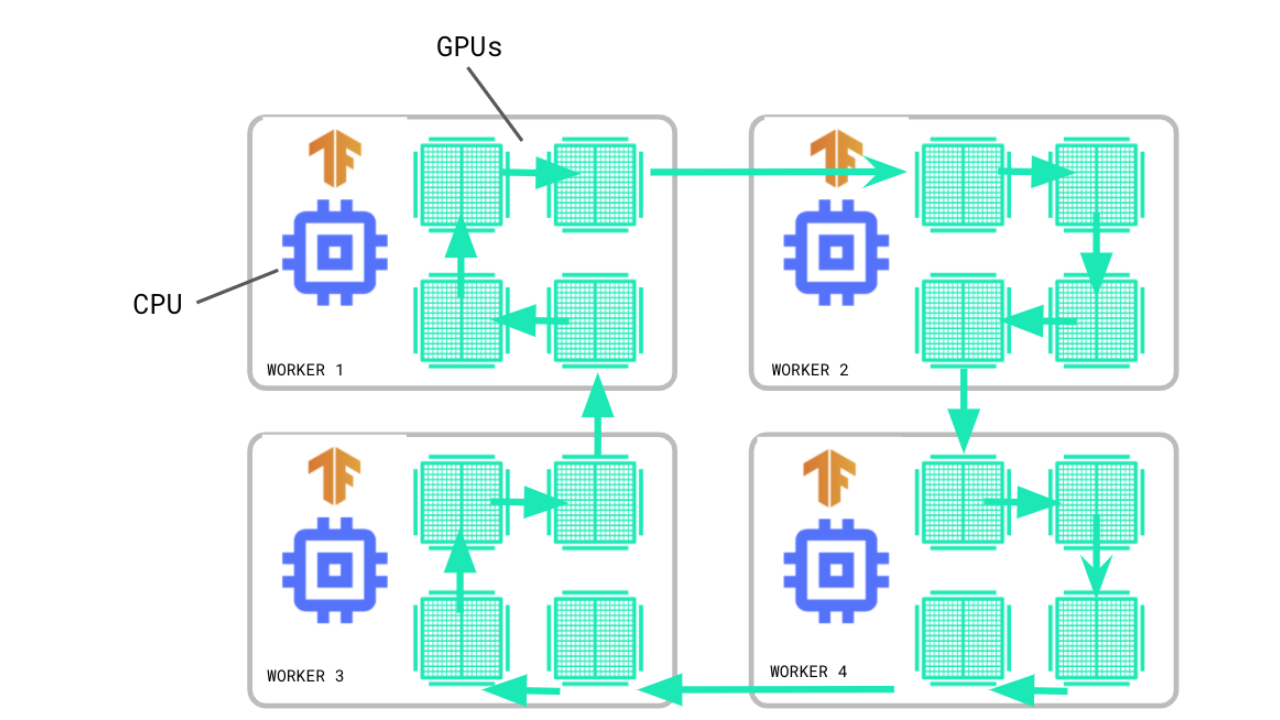
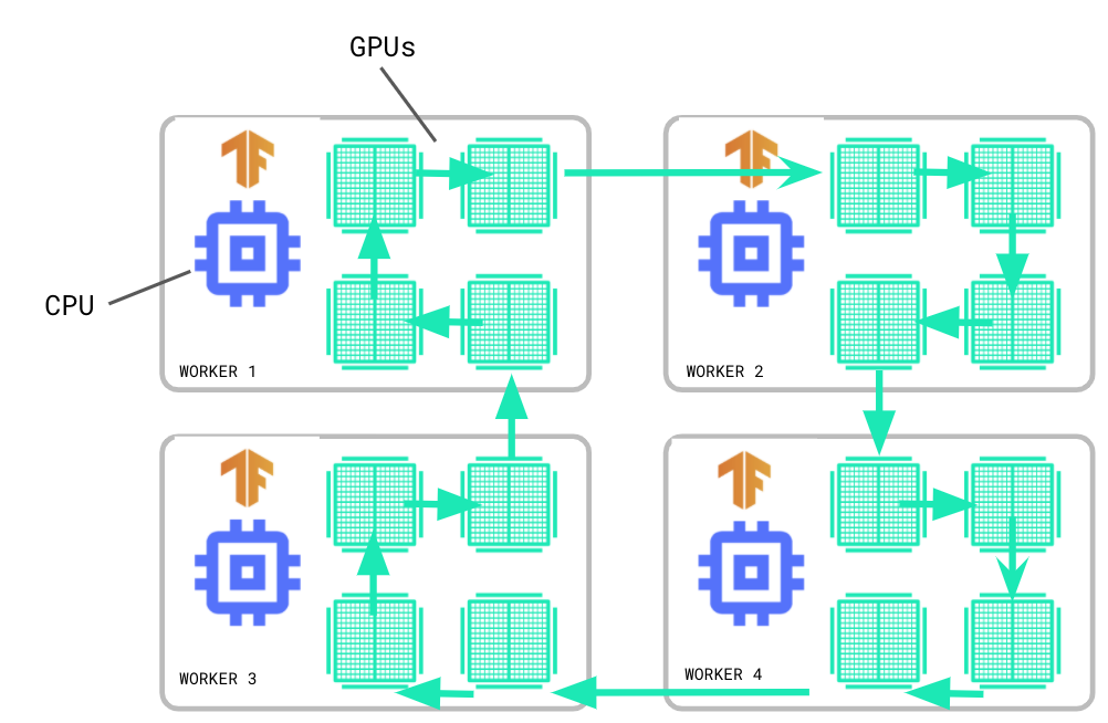
MultiWorkerMirroredStrategy has moved out of experimental and is now part of the stable API. Like its single worker counterpart, MirroredStrategy, MultiWorkerMirroredStrategy implements distributed training with synchronous data parallelism. However, as the name suggests, with MultiWorkerMirroredStrategy you can train across multiple machines, each with potentially multiple GPUs.

In synchronous training, each worker computes the forward and backward passes on different slices of the input data, and the gradients are aggregated before updating the model. For this aggregation, known as an all-reduce, MultiWorkerMirroredStrategy uses CollectiveOps to keep variables in sync. A collective op is a single op in the TensorFlow graph that can automatically choose an all-reduce algorithm in the TensorFlow runtime according to hardware, network topology, and tensor sizes.

Graph of TF GPUs and CPU

To get started with MultiWorkerMirroredStrategy, check out the Multi-worker training with Keras tutorial, which has been updated with details on dataset sharding, saving/loading models trained with a distribution strategy, and failure recovery with the BackupAndRestore callback.

If you are new to distributed training and want to learn how to get started, or you’re interested in distributed training on GCP, see this blog post for an introduction to the key concepts and steps.

Updates in Keras

Mixed Precision

In TensorFlow 2.4, the Keras mixed precision API has moved out of experimental and is now a stable API. Most TensorFlow models use the float32 dtype; however, there are lower-precision types such as float16 that use less memory. Mixed precision is the use of 16-bit and 32-bit floating point types in the same model for faster training. This API can improve model performance by 3x on GPUs and 60% on TPUs.

To make use of the mixed precision API, you must use Keras layers and optimizers, but it’s not necessary to use other Keras classes such as models or losses. If you’re curious to learn how to take advantage of this API for better performance, check out the Mixed Precision tutorial.

Optimizers

This release includes refactoring the tf.keras.optimizers.Optimizer class, enabling users of model.fit or custom training loops to write training code that works with any optimizer. All built-in tf.keras.optimizer.Optimizer subclasses now accept gradient_transformers and gradient_aggregator arguments, allowing you to easily define custom gradient transformations.

With the refactor, you can now pass a loss tensor directly to Optimizer.minimize when writing custom training loops:

tape = tf.GradientTape()
with tape:
y_pred = model(x, training=True)
loss = loss_fn(y_pred, y_true)

# You can pass in the `tf.GradientTape` when using a loss `Tensor` as shown below.

optimizer.minimize(loss, model.trainable_variables, tape=tape)

These changes are intended to make both Model.fit and custom training loops more agnostic to optimizer details, allowing you to write training code that works with any optimizer without modification.

Functional API model construction internal improvements

Lastly, TensorFlow 2.4 includes a major refactoring of the internals of the Keras Functional API, improving the memory consumption of functional model construction and simplifying triggering logic. This refactoring also ensures TensorFlowOpLayers behave predictably and work with CompositeTensor type signatures.

Introducing tf.experimental.numpy

TensorFlow 2.4 introduces experimental support for a subset of NumPy APIs, available as tf.experimental.numpy. This module enables you to run NumPy code, accelerated by TensorFlow. Because it is built on top of TensorFlow, this API interoperates seamlessly with TensorFlow, allowing access to all of TensorFlow’s APIs and providing optimized execution using compilation and auto-vectorization. For example, TensorFlow ND arrays can interoperate with NumPy functions, and similarly TensorFlow NumPy functions can accept inputs of different types including tf.Tensor and np.ndarray.

import tensorflow.experimental.numpy as tnp

# Use NumPy code in input pipelines

dataset = tf.data.Dataset.from_tensor_slices(
tnp.random.randn(1000, 1024)).map(
lambda z: z.clip(-1,1)).batch(100)

# Compute gradients through NumPy code

def grad(x, wt):
with tf.GradientTape() as tape:
tape.watch(wt)
output = tnp.dot(x, wt)
output = tf.sigmoid(output)
return tape.gradient(tnp.sum(output), wt)

You can learn more about how to use this API in the NumPy API on TensorFlow guide.

New Profiler Tools

MultiWorker Support in TensorFlow Profiler

The TensorFlow Profiler is a suite of tools you can use to measure the training performance and resource consumption of your TensorFlow models. The TensorFlow Profiler helps you understand the hardware resource consumption of the ops in your model, diagnose bottlenecks, and ultimately train faster.

Previously, the TensorFlow Profiler supported monitoring multi-GPU, single host training jobs. In 2.4 you can now profile MultiWorkerMirroredStrategy training jobs. For example, you can use the sampling mode API to perform on demand profiling and connect to the same server:port in use by MultiWorkerMirroredStrategy workers:


# Start a profiler server before your model runs.


tf.profiler.experimental.server.start(6009)

# Model code goes here....

# E.g. your worker IP addresses are 10.0.0.2, 10.0.0.3, 10.0.0.4, and you
# would like to profile for a duration of 2 seconds. The profiling data will
# be saved to the Google Cloud Storage path “your_tb_logdir”.

tf.profiler.experimental.client.trace(
'grpc://10.0.0.2:6009,grpc://10.0.0.3:6009,grpc://10.0.0.4:6009',
'gs://your_tb_logdir',
2000)

Alternatively, you can use the TensorBoard profile plugin by providing the worker addresses to the Capture Profile tool.

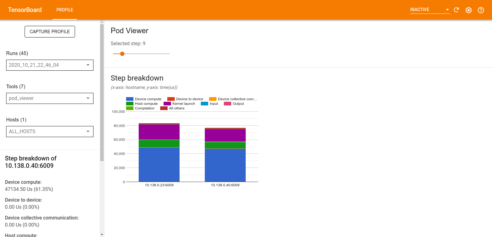
After profiling, you can use the new Pod Viewer tool to choose a training step and view its step-time category breakdown across all workers.

TensorBoard preview

For more information on how to use the TensorFlow Profiler, check out the newly released GPU Performance Guide. This guide shows common scenarios you might encounter when you profile your model training job and provides a debugging workflow to help you get better performance, whether you’re training with one GPU, multiple GPUs, or multiple machines.

TFLite Profiler

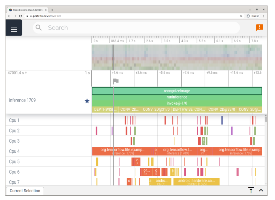
The TFLite Profiler enables tracing TFLite internals in Android to identify performance bottlenecks. The TFLite Performance Measurement Guide shows you how to add trace events, enable TFLite tracing, and capture traces with both the Android Studio CPU Profiler and the System Tracing app.

Example trace using the Android System Tracing app

Example trace using the Android System Tracing app

New Features for GPU Support

TensorFlow 2.4 runs with CUDA 11 and cuDNN 8, enabling support for the newly available NVIDIA Ampere GPU architecture. To learn more about CUDA 11 features, check out this NVIDIA developer blog.

Additionally, support for TensorFloat-32 on Ampere-based GPUs is enabled by default. TensorFloat-32, or `TF32` for short, is a math mode for NVIDIA Ampere GPUs that causes certain float32 ops, such as matrix multiplications and convolutions, to run much faster on Ampere GPUs but with reduced precision. To learn more , see the documentation for tf.config.experimental.enable_tensor_float_32_execution.

Next steps

Check out the release notes for more information. To stay up to date, you can read the TensorFlow blog, follow twitter.com/tensorflow, or subscribe to youtube.com/tensorflow. If you’ve built something you’d like to share, please submit it for our Community Spotlight at goo.gle/TFCS. For feedback, please file an issue on GitHub. Thank you!

Read More

Representational Aspects of Depth and Conditioning in Normalizing Flows

Representational Aspects of Depth and Conditioning in Normalizing Flows

Top and Bottom Right: RealNVP [3] uses checkerboard and channel-wise partitioning schemes in order to factor out parameters and ensure that there aren’t redundant partitions from previous layers. GLOW [4] uses an invertible 1×1 convolution which allows the partitioned to be ‘learned’ by a linear layer. We show that arbitrary partitions can be simulated in a constant number of layers with a fixed partition, showing that these ideas increase representational power by at most a constant factor. Bottom Left: Random points are well-separated with high probability on a high-dimensional sphere, which allows us to construct a distribution that is challenging for flows.

The promise of unsupervised learning lies in its potential to take advantage of cheap and plentiful unlabeled data to learn useful representations or generate high-quality samples. For the latter task, neural network-based generative models have recently enjoyed a lot of success in producing realistic images and text. Two major paradigms in deep generative modeling are generative adversarial networks (GANs) and normalizing flows. When successfully scaled up and trained, both can generate high-quality and diverse samples from high-dimensional distributions. The training procedure for GANs involves min-max (saddle-point) optimization, which is considerably more difficult than standard loss minimization, leading to problems like mode dropping.

Samples from a GLOW [4] model trained on the CelebA Faces Dataset.

Normalizing flows [1] have been proposed as an alternative type of generative model which allows not only efficient sampling but also training via maximum likelihood through a closed-form computation of the likelihood function. They are written as pushforwards of a simple distribution (typically a Gaussian) through an invertible transformation (f), typically parametrized as a composition of simple invertible transformations. The main reason for this parametrization is the change-of-variables formula: if (z) is a random variable sampled from a known base distribution (P(z)) (typically a standard multivariate normal), (f: mathbb{R}^dto mathbb{R}^d) is invertible and differentiable, and (x = f^{-1}(z)) then $$p(x) = p(f(x))left|detleft(frac{partial f(x)}{partial x^T}right)right|.$$ Here, (frac{partial f(x)}{partial x^T}) is the Jacobian of (f).

Normalizing flows are trained by maximizing the likelihood using gradient descent. However, in practice, training normalizing flows runs into difficulties as well: models which produce good samples typically need to be extremely deep — which comes with accompanying vanishing/exploding gradient problems. A very related problem is that they are often poorly conditioned. Data like images are often inherently lower-dimensional than the ambient space, the map from low dimensional data to high dimensional latent variables can be difficult to invert and therefore train.

In our recent work [2], we tackle representational questions around depth and conditioning of normalizing flows—first for general invertible architectures, then for a particular common architecture—where the normalizing flow is a composition of so-called affine couplings.

Depth Bound on General Invertible Architectures

The most fundamental restriction of the normalizing flow paradigm is that each layer needs to be invertible. We ask whether this restriction has any ‘cost’ in terms of the size, and in particular the depth, of the model. Here we’re counting depth in terms of the number of the invertible transformations that make up the flow. A requirement for large depth would explain training difficulties due to exploding (or vanishing) gradients.

Since the Jacobian of a composition of functions is the product of the Jacobians of the functions being composed, the min (max) singular value of the Jacobian of the composition is the product of the min (max) singular value of the Jacobians of the functions. This implies that the smallest (largest) singular value of the Jacobian will get exponentially smaller (larger) with the number of compositions.

A natural way of formalizing this question is by exhibiting a distribution which is easy to model for an unconstrained generator network but hard for a shallow normalizing flow. Precisely, we ask: is there a probability distribution that can be represented by a shallow generator with a small number of parameters that could not be approximately represented by a shallow composition of invertible transformations?

We demonstrate that such a distribution exists. Specifically, we show that

Theorem: For every k, s.t. (k = o(exp(d))) and any parameterized family of compositions of Lipschitz invertible transformations with (p) parameters per transformation and at most (O(k / p)) transformations, there exists a generator (g:mathbb{R}^{d+1} to mathbb{R}) with depth (O(1)) and (O(k)) parameters s.t the pushforward of a Gaussian through (g) cannot be approximated in either KL or Wasserstein-1 distance by a network in this family.

The result above is extremely general: it only requires a bound on the number of parameters per transformation in the parametrization of the normalizing flow and Lipschitzness of these maps. As such it easily includes common choices used in practice like affine couplings with at most (p) parameters per layer or invertible feedforward networks, where each intermediate layer is of dimension (d) and the nonlinearity is invertible (e.g. leaky ReLU). On the flip side, for possible architectures with a large number of parameters per transformation, this theorem gives a (possibly loose) lower bound of a small number of transformations.

Proof Sketch: The generator for our construction approximates a mixture of (k) Gaussians with means placed uniformly randomly on a (d)-dimensional sphere in the ambient space. We will use the probabilistic method to show there is a family of such mixtures, s.t. each pair of members in this family are far apart (say, in Wasserstein distance). Furthermore, by an epsilon net discretization argument we can count how many “essentially” distinct invertible Lipschitz networks there are. If the number of mixtures in the family is much larger than the size of the epsilon net, at least one mixture must be far from all invertible networks.

We choose well-separated modes on a hypersphere in order to generate a large family of well separated mixtures of Gaussians.

The family of mixtures is constructed by choosing the (k) means for the components uniformly at random on a sphere. It’s well known that (exp(o(d))) randomly chosen points on a unit sphere will, with high probability, have constant pairwise distance. Similarly, coding-theoretic arguments (used to prove the so-called Gilbert-Varshamov bound) can be used to show that selecting (exp(o(d))) (k)-tuples of those means will, with high probability, ensure that each pair of (k)-tuples is such that the average pair of means is at constant distance. This suffices to ensure the Wasserstein distance between pairs of mixtures is large. ∎

Results for Affine Couplings

Affine Couplings [3] are one of the most common transformations in scalable architectures for normalizing flows. An affine coupling is a map (f: mathbb{R}^dto mathbb{R}^d) such that for some partition into a set containing approximately half of the coordinates (S) and it’s complement, $$f(x_S, x_{[d]setminus S}) = (x_S, x_{[d]setminus S} odot s(x_s) + t(x_s))$$ for some scaling and translation functions (typically parameterized by neural networks) (s) and (t). Clearly, an affine coupling block only transforms one partition of the coordinates at a time by an affine function while leaving the other partition intact. It’s easy to see that an affine coupling is invertible if each coordinate of (s) is invertible. Moreover, the Jacobian of this function is $$begin{bmatrix}I & 0\frac{partial t}{partial x_S^T} & text{diag}(s(x_S))end{bmatrix}$$ In particular it’s lower triangular, so we can calculate the determinant in linear time by multiplying the (d) diagonal elements (in general determinants take (O(d^3)) time to compute). This allows us to efficiently compute likelihoods and their gradients for SGD on large models via the change of variables formula.
These affine coupling blocks are stacked, often while changing the part of the partition that is updated or more generally, permuting the elements in between the application of the coupling.

Affine couplings consist of nonlinear affine transformations of half of the data dimensions at a time which end in a normal distribution. We show that the choice of which dimensions are in which half can be simulated in a constant number of couplings. Source

Effect of the Choice of Partition on Representational Power

Partitions in Real NVP. Source

The choice of partition is often somewhat ad-hoc and involves domain knowledge (e.g. for image datasets, a typical choice is a checkerboard pattern or a channel-wise partition). In fact, some recent approaches like GLOW [4] try to “learn” permutations to apply between each pair of affine couplings. (Technically, since a permutation is a discrete object, in [4] the authors learn a 1×1 convolutions instead.)

While ablation experiments provide definite evidence that including learned 1×1 convolutions is beneficial for modeling image data in practice, it’s unclear whether this effect is from increased modeling power or algorithmic effects — and even less so how to formally quantify it. In this section, we come to a clear understanding of the representational value of adding this flexibility in partitioning. We knew from GLOW that adding these partitions helped. Now we know why!

We formalize the representational question as follows: how many affine couplings with a fixed partition are needed to simulate an arbitrary linear map? Since a linear map is more general than a 1×1 convolution, if it’s possible to do so with a small (say constant) number of affine couplings, we can simulate any affine coupling-based normalizing flow including 1×1 convolutions by one that does not include them which is merely a constant factor larger.

Concretely, we consider linear functions of the form $$T = prod_{i=1}^Kbegin{bmatrix}I & 0\A_i & B_iend{bmatrix} begin{bmatrix}C_i & D_i\0 & Iend{bmatrix},$$ for matrices (A_i, D_i in mathbb{R}^{dtimes d}) and diagonal matrices (B_i, C_i in mathbb{R}^{dtimes d}). The right hand side is precisely a composition of affine coupling blocks with linear maps (s, t) with a fixed partition (the parts of the input that are being updated alternate). We show the following result:

Theorem: To represent an arbitrary invertible (T), (K) must be at most 24. Additionally, there exist invertible matrices (T) such that (K geq 3).

Proof sketch: The statement hopefully reminds the reader of the standard LU decomposition — the twist of course being that the matrices on the right-hand side have a more constrained structure than merely being triangular. Our proof starts with the existence of a (LUP) decomposition for every matrix.

We first show that we can construct an arbitrary permutation (up to sign) using at most 21 alternating matrices of the desired form. The argument is group theoretic: we use the fact that a permutation decomposes into a composition of two permutations of order 2, which must be disjoint products of swaps and show that swapping elements can be implemented “in parallel” using several partitioned matrices of the type we’re considering.

Next, we show that we can produce an arbitrary triangular matrix with our partitioned matrices. We use similar techniques as above to reduce the matrix to a regular system of block linear equations which we can then solve. Our upper bound comes from just counting the total number of matrices required for these operations: the 21 for the permutation and 13 for each triangular matrix (upper and lower), giving a total of 47 required matrices. ∎

To reiterate the takeaway: a GLOW-style linear layer in between affine couplings could in theory make your network between 5 and 47 times smaller while representing the same function. We now have a precise understanding of the value of that architectural choice!

We also verified empirically in the figure below how well these linear models would fit randomly chosen (i.e. with iid Gaussian entries) linear functions. It seems empirically that at least for this ensemble our upper bound is loose and we can fit the functions well without using the full 47 layers. Closing this gap is an interesting problem for future work.

We regress affine couplings with linear scaling and translation functions at a variety of depths on linear functions determined by random matrices. It seems like we can fit these functions arbitrarily well with 4-16 layers, suggesting that at least in random cases the true number of layers required is closer to our lower bound.

Universal Approximation with Poorly Conditioned Networks

In our earlier result on the depth of invertible networks, we assumed that our network was Lipschitz and therefore well-conditioned. A natural question is then, if we remove this requirement, how powerful is the resulting class of models? In particular, we ask: are poorly conditioned affine coupling-based normalizing flows universal approximators as they are used in practice?

Curiously, this question has in fact not been answered in prior work. In a very recent work [5], it was shown that if we allow for padding of our data with extra dimensions that take a constant value 0, affine couplings are universal approximators. (Note, this kind of padding clearly results in a singular Jacobian — as the value in the added dimensions is constant.) The idea for why padding helps is that these extra dimensions are used as a “scratch pad” for the computation the network is performing. Another recent work [6] gives a proof of universal approximation for affine couplings assuming arbitrary permutations in between the layers are allowed (ala Glow) and a partition separating (d -1) dimensions from the other. However, in practice, these models are trained using a roughly half-half split and often without linear layers in between couplings (which already works quite well). We prove that none of these architectural modifications to affine couplings are necessary for universal approximation and additionally suggest a trade-off between the conditioning of the model and the quality of its approximation. Concretely, we show:

Theorem: For any bounded and absolutely continuous distribution (Q) over (mathbb{R}^n) and any (epsilon > 0), there exists a 3-layer affine coupling (g) with maps (s, t) represented by feedforward ReLU networks such that (W_2(g_# P, Q) leq epsilon), where (g_# P) is the pushforward of a standard Gaussian through (g).

We note that the construction for the theorem trades off quality of approximation ((epsilon)) with conditioning: the smallest singular value of the Jacobian in the construction for our theorem above will scale like (1/epsilon) — thus suggesting that if we want to use affine couplings as universal approximators, conditioning may be an issue even if we don’t pad with a constant value for the added dimensions like prior works — which obviously results in a singular Jacobian.

Proof sketch: The proof is based on two main ideas.

The first is a deep result from optimal transport, Brenier’s theorem, which for sufficiently “regular” distributions (p) over (mathbb{R}^d) guarantees an invertible map (phi), s.t. the pushforward of the Gaussian through (phi) equals (p). This reduces our problem to approximating (phi) using a sequence of affine couplings.

The difficulty in approximating (phi) is the fact that affine couplings are only allowed to change one part of the input, and in a constrained way. The trick we use to do this without a “scratchpad” to store intermediate computation as in prior works is to instead hide information in the “low order bits” of the other partition. For details, refer to our paper. ∎

Finally, on the experimental front, we wanted to experiment with how padding affects the conditioning of a learned model. We considered synthetic 2d datasets (see figure below) and found that padding with zeros resulted in a very poorly conditioned model which produced poor samples, as might be expected. We also considered a type of padding which is reasonable but for which we have no theory — namely, to use iid Gaussian samples as values for the added dimensions (in this case, the resulting Jacobians are not prima facie singular, and the model can still use them as a “scratch pad”). While we have no result that this in any formal sense can result in better-conditioned networks, we found that in practice it frequently does and it also results in better samples. This seems like a very fruitful direction for future research. Finally, without padding, the model produces samples of middling quality and has a condition number in between that of zero and Gaussian padding.

In both examples, Gaussian padding of the data gives a sharper distribution and a better-conditioned model.

Conclusions

Normalizing flows are one of the most popular generative models across various domains, though we still have a relatively narrow understanding of their relative pros and cons compared to other models. We show in this work that there are fundamental tradeoffs between depth and conditioning and representational power of this type of function. Though we have cleared up considerably the representational aspects of these models, the algorithmic and statistical questions are still wide open. We hope that this work guides both users of flows and theoreticians as to the fine-grained properties of flows as compared to other generative models.

Bibliography

[1] Rezende and Mohamed, 2015, Variational Inference with Normalizing Flows, ICML 2015

[2] Koehler, Mehta, and Risteski, 2020, Representational aspects of depth and conditioning in normalizing flows, Under Submission.

[3] Dinh, Sohl-Dickstein, and S. Bengio, 2016, Density estimation using Real NVP, ICLR 2016

[4] Kingma and Dhariwal, 2018, GLOW: Generative flow with 1×1 convolutions, NeurIPS 2018

[5] Huang, Dinh, and Courville, 2020, Augmented Normalizing Flows: Bridging the Gap Between Generative Flows and Latent Variable Models

[6] Teshima, Ishikawa, Tojo, Oono, Ikeda, and Sugiyama, 2020, Coupling-based Invertible Neural Networks Are Universal Diffeomorphism Approximators, NeurIPS 2020

Read More

Stuttgart Supercomputing Center Shifts into AI Gear

Stuttgart Supercomputing Center Shifts into AI Gear

Stuttgart’s supercomputer center has been cruising down the autobahn of high performance computing like a well-torqued coupe, and now it’s making a pitstop for some AI fuel.

Germany’s High-Performance Computing Center Stuttgart (HLRS), one of Europe’s largest supercomputing centers, has tripled the size of its staff and increased its revenues from industry collaborations 20x since Michael Resch became director in 2002. In the past year, much of the growth has come from interest in AI.

With demand for machine learning on the rise, HLRS signed a deal to add 192 NVIDIA Ampere architecture GPUs linked on NVIDIA Mellanox InfiniBand network to its Hawk supercomputer based on an Apollo system from Hewlett Packard Enterprise.

Hawk Flies to New Heights

The GPUs will propel what’s already ranked as the world’s 16th largest system to new heights. In preparation for the expansion, researchers are gearing up AI projects that range from predicting the path of the COVID-19 pandemic to the science behind building better cars and planes.

“Humans can create huge simulations, but we can’t always understand all the data — the big advantage of AI is it can work through the data and see its consequences,” said Resch, who also serves as a professor at the University of Stuttgart with a background in engineering, computer science and math.

The center made its first big leap into AI last year when it installed a Cray CS-Storm system with more than 60 NVIDIA GPUs. It is already running AI programs that analyze market data for Mercedes-Benz, investment portfolios for a large German bank and a music database for a local broadcaster.

“It turned out to be an extremely popular system because there’s a growing community of people who understand AI has a benefit for them,” Resch said of the system now running at near capacity. “By the middle of this year it was clear we had to expand to cover our growing AI requirements,” he added.

The New Math: HPC+AI

The future for the Stuttgart center, and the HPC community generally, is about hybrid computing where CPUs and GPUs work together, often to advance HPC simulations with AI.

“Combining the two is a golden bullet that propels us into a better future for understanding problems,” he said.

For example, one researcher at the University of Stuttgart will use data from as many as 2 billion simulations to train neural networks that can quickly and economically evaluate metal alloys. The AI model it spawns could run on a PC and help companies producing sheet metal choose the best alloys for, say, a car door.

“This is extremely helpful in situations where experimentation is difficult or costly,” he said.

And it’s an apropos app for the center situated in the same city that’s home to the headquarters of both Mercedes and Porsche.

In the Flow with Machine Learning

A separate project in fluid dynamics will take a similar approach.

A group from the university will train neural networks on data from highly accurate simulations to create an AI model that can improve analysis of turbulence. It’s a critical topic for companies such as Airbus that are collaborating with HLRS on efforts to mine the aerospace giant’s data on airflow.

The Stuttgart center also aims to use AI as part of a European research project to predict when hospital beds could fill up in intensive-care units amid the pandemic. The project started before the coronavirus hit, but it accelerated in the wake of COVID-19.

Tracking the Pandemic with AI

One of the project’s goals is to give policy makers a four-week window to respond before hospitals would reach their capacity.

“It’s a critical question with so many people dying — we’ve seen scenarios in places like Italy, New York and Wuhan where ICUs filled up in the first weeks of pandemic,” Resch said.

“So, we will conduct simulations and predictions of the outlook for the pandemic over the next weeks and months, and GPUs will be extremely helpful for that,” he added.

It’s perhaps the highest profile of many apps now in the pipeline for the GPU-enhanced engine that will propel Stuttgart’s researchers further down the road on their journey into AI.

The post Stuttgart Supercomputing Center Shifts into AI Gear appeared first on The Official NVIDIA Blog.

Read More

Portrait Light: Enhancing Portrait Lighting with Machine Learning

Portrait Light: Enhancing Portrait Lighting with Machine Learning

Posted by Yun-Ta Tsai1 and Rohit Pandey, Software Engineers, Google Research

Professional portrait photographers are able to create compelling photographs by using specialized equipment, such as off-camera flashes and reflectors, and expert knowledge to capture just the right illumination of their subjects. In order to allow users to better emulate professional-looking portraits, we recently released Portrait Light, a new post-capture feature for the Pixel Camera and Google Photos apps that adds a simulated directional light source to portraits, with the directionality and intensity set to complement the lighting from the original photograph.

Example image with and without Portrait Light applied. Note how Portrait Light contours the face, adding dimensionality, volume, and visual interest.

In the Pixel Camera on Pixel 4, Pixel 4a, Pixel 4a (5G), and Pixel 5, Portrait Light is automatically applied post-capture to images in the default mode and to Night Sight photos that include people — just one person or even a small group. In Portrait Mode photographs, Portrait Light provides more dramatic lighting to accompany the shallow depth-of-field effect already applied, resulting in a studio-quality look. But because lighting can be a personal choice, Pixel users who shoot in Portrait Mode can manually re-position and adjust the brightness of the applied lighting within Google Photos to match their preference. For those running Google Photos on Pixel 2 or newer, this relighting capability is also available for many pre-existing portrait photographs.

Pixel users can adjust a portrait’s lighting as they like in Google Photos, after capture.

Today we present the technology behind Portrait Light. Inspired by the off-camera lights used by portrait photographers, Portrait Light models a repositionable light source that can be added into the scene, with the initial lighting direction and intensity automatically selected to complement the existing lighting in the photo. We accomplish this by leveraging novel machine learning models, each trained using a diverse dataset of photographs captured in the Light Stage computational illumination system. These models enabled two new algorithmic capabilities:

  1. Automatic directional light placement: For a given portrait, the algorithm places a synthetic directional light in the scene consistent with how a photographer would have placed an off-camera light source in the real world.
  2. Synthetic post-capture relighting: For a given lighting direction and portrait, synthetic light is added in a way that looks realistic and natural.

These innovations enable Portrait Light to help create attractive lighting at any moment for every portrait — all on your mobile device.

Automatic Light Placement
Photographers usually rely on perceptual cues when deciding how to augment environmental illumination with off-camera light sources. They assess the intensity and directionality of the light falling on the face, and also adjust their subject’s head pose to complement it. To inform Portrait Light’s automatic light placement, we developed computational equivalents to these two perceptual signals.

First, we trained a novel machine learning model to estimate a high dynamic range, omnidirectional illumination profile for a scene based on an input portrait. This new lighting estimation model infers the direction, relative intensity, and color of all light sources in the scene coming from all directions, considering the face as a light probe. We also estimate the head pose of the portrait’s subject using MediaPipe Face Mesh.

Estimating the high dynamic range, omnidirectional illumination profile from an input portrait. The three spheres at the right of each image, diffuse (top), matte silver (middle), and mirror (bottom), are rendered using the estimated illumination, each reflecting the color, intensity, and directionality of the environmental lighting.

Using these clues, we determine the direction from which the synthetic lighting should originate. In studio portrait photography, the main off-camera light source, or key light, is placed about 30° above the eyeline and between 30° and 60° off the camera axis, when looking overhead at the scene. We follow this guideline for a classic portrait look, enhancing any pre-existing lighting directionality in the scene while targeting a balanced, subtle key-to-fill lighting ratio of about 2:1.

Data-Driven Portrait Relighting
Given a desired lighting direction and portrait, we next trained a new machine learning model to add the illumination from a directional light source to the original photograph. Training the model required millions of pairs of portraits both with and without extra light. Photographing such a dataset in normal settings would have been impossible because it requires near-perfect registration of portraits captured across different lighting conditions.

Instead, we generated training data by photographing seventy different people using the Light Stage computational illumination system. This spherical lighting rig includes 64 cameras with different viewpoints and 331 individually-programmable LED light sources. We photographed each individual illuminated one-light-at-a-time (OLAT) by each light, which generates their reflectance field — or their appearance as illuminated by the discrete sections of the spherical environment. The reflectance field encodes the unique color and light-reflecting properties of the subject’s skin, hair, and clothing — how shiny or dull each material appears. Due to the superposition principle for light, these OLAT images can then be linearly added together to render realistic images of the subject as they would appear in any image-based lighting environment, with complex light transport phenomena like subsurface scattering correctly represented.

Using the Light Stage, we photographed many individuals with different face shapes, genders, skin tones, hairstyles, and clothing/accessories. For each person, we generated synthetic portraits in many different lighting environments, both with and without the added directional light, rendering millions of pairs of images. This dataset encouraged model performance across diverse lighting environments and individuals.

Photographing an individual as illuminated one-light-at-a-time in the Google Light Stage, a 360° computational illumination rig.
Left: Example images from an individual’s photographed reflectance field, their appearance in the Light Stage as illuminated one-light-at-a-time. Right: The images can be added together to form the appearance of the subject in any novel lighting environment.

Learning Detail-Preserving Relighting Using the Quotient Image
Rather than trying to directly predict the output relit image, we trained the relighting model to output a low-resolution quotient image, i.e., a per-pixel multiplier that when upsampled can be applied to the original input image to produce the desired output image with the contribution of the extra light source added. This technique is computationally efficient and encourages only low-frequency lighting changes, without impacting high-frequency image details, which are directly transferred from the input to maintain image quality.

Supervising Relighting with Geometry Estimation
When photographers add an extra light source into a scene, its orientation relative to the subject’s facial geometry determines how much brighter each part of the face appears. To model the optical behavior of light sources reflecting off relatively matte surfaces, we first trained a machine learning model to estimate surface normals given the input photograph, and then applied Lambert’s law to compute a “light visibility map” for the desired lighting direction. We provided this light visibility map as input to the quotient image predictor, ensuring that the model is trained using physics-based insights.

The pipeline of our relighting network. Given an input portrait, we estimate per-pixel surface normals, which we then use to compute a light visibility map. The model is trained to produce a low-resolution quotient image that, when upsampled and applied as a multiplier to the original image, produces the original portrait with an extra light source added synthetically into the scene.

We optimized the full pipeline to run at interactive frame-rates on mobile devices, with total model size under 10 MB. Here are a few examples of Portrait Light in action.

Portrait Light in action.

Getting the Most Out of Portrait Light
You can try Portrait Light in the Pixel Camera and change the light position and brightness to your liking in Google Photos. For those who use Dual Exposure Controls, Portrait Light can be applied post-capture for additional creative flexibility to find just the right balance between light and shadow. On existing images from your Google Photos library, try it where faces are slightly underexposed, where Portrait Light can illuminate and highlight your subject. It will especially benefit images with a single individual posed directly at the camera.

We see Portrait Light as the first step on the journey towards creative post-capture lighting controls for mobile cameras, powered by machine learning.

Acknowledgements
Portrait Light is the result of a collaboration between Google Research, Google Daydream, Pixel, and Google Photos teams. Key contributors include: Yun-Ta Tsai, Rohit Pandey, Sean Fanello, Chloe LeGendre, Michael Milne, Ryan Geiss, Sam Hasinoff, Dillon Sharlet, Christoph Rhemann, Peter Denny, Kaiwen Guo, Philip Davidson, Jonathan Taylor, Mingsong Dou, Pavel Pidlypenskyi, Peter Lincoln, Jay Busch, Matt Whalen, Jason Dourgarian, Geoff Harvey, Cynthia Herrera, Sergio Orts Escolano, Paul Debevec, Jonathan Barron, Sofien Bouaziz, Clement Ng, Rachit Gupta, Jesse Evans, Ryan Campbell, Sonya Mollinger, Emily To, Yichang Shih, Jana Ehmann, Wan-Chun Alex Ma, Christina Tong, Tim Smith, Tim Ruddick, Bill Strathearn, Jose Lima, Chia-Kai Liang, David Salesin, Shahram Izadi, Navin Sarma, Nisha Masharani, Zachary Senzer.


1  Work conducted while at Google. 

Read More

Exploratory data analysis, feature engineering, and operationalizing your data flow into your ML pipeline with Amazon SageMaker Data Wrangler

Exploratory data analysis, feature engineering, and operationalizing your data flow into your ML pipeline with Amazon SageMaker Data Wrangler

According to The State of Data Science 2020 survey, data management, exploratory data analysis (EDA), feature selection, and feature engineering accounts for more than 66% of a data scientist’s time (see the following diagram).

According to The State of Data Science 2020 survey, data management, exploratory data analysis (EDA), feature selection, and feature engineering accounts for more than 66% of a data scientist’s time.

The same survey highlights that the top three biggest roadblocks to deploying a model in production are managing dependencies and environments, security, and skill gaps (see the following diagram).

The same survey highlights that the top three biggest roadblocks to deploying a model in production are managing dependencies and environments, security, and skill gaps.

The survey posits that these struggles result in fewer than half (48%) of the respondents feeling able to illustrate the impact data science has on business outcomes.

Enter Amazon SageMaker Data Wrangler, the fastest and easiest way to prepare data for machine learning (ML). SageMaker Data Wrangler gives you the ability to use a visual interface to access data, perform EDA and feature engineering, and seamlessly operationalize your data flow by exporting it into an Amazon SageMaker pipeline, Amazon SageMaker Data Wrangler job, Python file, or SageMaker feature group.

SageMaker Data Wrangler also provides you with over 300 built-in transforms, custom transforms using a Python, PySpark or SparkSQL runtime, built-in data analysis such as common charts (like scatterplot or histogram), custom charts using the Altair library, and useful model analysis capabilities such as feature importance, target leakage, and model explainability. Finally, SageMaker Data Wrangler creates a data flow file that can be versioned and shared across your teams for reproducibility.

Solution overview

In this post, we use the retail demo store example and generate a sample dataset. We use three files: users.csv, items.csv, and interactions.csv. We first prepare the data in order to predict the customer segment based on past interactions. Our target is the field called persona, which we later transform and rename to USER_SEGMENT.

The following code is a preview of the users dataset:

id,username,email,first_name,last_name,addresses,age,gender,persona
1,user1,nathan.smith@example.com,Nathan,Smith,"[{""first_name"": ""Nathan"", ""last_name"": ""Smith"", ""address1"": ""049 Isaac Stravenue Apt. 770"", ""address2"": """", ""country"": ""US"", ""city"": ""Johnsonmouth"", ""state"": ""NY"", ""zipcode"": ""12758"", ""default"": true}]",28,M,electronics_beauty_outdoors
2,user2,kevin.martinez@example.com,Kevin,Martinez,"[{""first_name"": ""Kevin"", ""last_name"": ""Martinez"", ""address1"": ""074 Jennifer Flats Suite 538"", ""address2"": """", ""country"": ""US"", ""city"": ""East Christineview"", ""state"": ""MI"", ""zipcode"": ""49758"", ""default"": true}]",19,M,electronics_beauty_outdoors

The following code is a preview of the items dataset:

ITEM_ID,ITEM_URL,ITEM_SK,ITEM_NAME,ITEM_CATEGORY,ITEM_STYLE,ITEM_DESCRIPTION,ITEM_PRICE,ITEM_IMAGE,ITEM_FEATURED,ITEM_GENDER_AFFINITY
36,http://dbq4nocqaarhp.cloudfront.net/#/product/36,,Exercise Headphones,electronics,headphones,These stylishly red ear buds wrap securely around your ears making them perfect when exercising or on the go.,19.99,5.jpg,true,
49,http://dbq4nocqaarhp.cloudfront.net/#/product/49,,Light Brown Leather Lace-Up Boot,footwear,boot,Sturdy enough for the outdoors yet stylish to wear out on the town.,89.95,11.jpg,,

The following code is a preview of the interactions dataset:

ITEM_ID,USER_ID,EVENT_TYPE,TIMESTAMP
2,2539,ProductViewed,1589580300
29,5575,ProductViewed,1589580305
4,1964,ProductViewed,1589580309
46,5291,ProductViewed,1589580309

This post is not intended to be a step-by-step guide, but rather describe the process of preparing a training dataset and highlight some of the transforms and data analysis capabilities using SageMaker Data Wrangler. You can download the .flow files if you want to download, upload, and retrace the full example in your SageMaker Studio environment.

At a high level, we perform the following steps: 

  1. Connect to Amazon Simple Storage Service (Amazon S3) and import the data.
  2. Transform the data, including type casting, dropping unneeded columns, imputing missing values, label encoding, one hot encoding, and custom transformations to extract elements from a JSON formatted column.
  3. Create table summaries and charts for data analysis. We use the quick model option to get a sense of which features are adding predictive power as we progress with our data preparation. We also use the built-in target leakage capability and get a report on any features that are at risk of leaking.
  4. Create a data flow, in which we combine and join the three tables to perform further aggregations and data analysis.
  5. Iterate by performing additional feature engineering or data analysis on the newly added data.
  6. Export our workflow to a SageMaker Data Wrangler job.

Prerequisites

Make sure you don’t have any quota limits on the m5.4xlarge instance type part of your Studio application before creating a new data flow. For more information about prerequisites, see Getting Started with Data Wrangler.

Importing the data

We import our three CSV files from Amazon S3. SageMaker Data Wrangler supports CSV and Parquet files. It also allows you to sample the data in case the data is too large to fit in your studio application. The following screenshot shows a preview of the users dataset.

A preview of the users dataset.

After importing our CSV files, our datasets look like the following screenshot in SageMaker Data Wrangler.

After importing our CSV files, our datasets look like the following screenshot in SageMaker Data Wrangler.

We can now add some transforms and perform data analysis.

Transforming the data

For each table, we check the data types and make sure that it was inferred correctly.

Items table

To perform transforms on the items table, complete the following steps:

  1. On the SageMaker Data Wrangler UI, for the items table, choose +.
  2. Choose Edit data types.

On the SageMaker Data Wrangler UI, for the items table, choose +.

Most of the columns were inferred properly, except for one. The ITEM_FEATURED column is missing values and should really be casted as a Boolean.

The ITEM_FEATURED column is missing values and should really be casted as a Boolean.

For the items table, we perform the following transformations:

  • Fill missing values with false for the ITEM_FEATURED column
  • Drop unneeded columns such as URL, SK, IMAGE, NAME, STYLE, ITEM_FEATURED and DESCRIPTION
  • Rename ITEM_FEATURED_IMPUTED to ITEM_FEATURED
  • Cast the ITEM_FEATURED column as Boolean
  • Encode the ITEM_GENDER_AFFINITY column
  1. To add a new transform, choose + and choose Add transform.

To add a new transform, choose + and choose Add transform.

  1. Fill in missing values using the built-in Handling missing values transform.

Fill in missing values using the built-in Handling missing values transform.

  1. To drop columns, under Manage columns, For Input column, choose ITEM_URL.
    1. For Required column operator, choose Drop column.
    2. Repeat this step for SK, IMAGE, NAME, STYLE, ITEM_FEATURED, and DESCRIPTION
  1. Under Type Conversion, for Column, choose ITEM_FEATURED.
  2. for To, choose Boolean.

  1. Under Encore categorical, add a one hot encoding transform to the ITEM_GENDER_AFFINITY column.

  1. Rename our column from ITEM_FEATURED_IMPUTED to ITEM_FEATURED.
  2. Run a table summary.

Rename our column from ITEM_FEATURED_IMPUTED to ITEM_FEATURED.

The table summary data analysis doesn’t provide information on all the columns.

  1. Run the df.info() function as a custom transform.
  2. Choose Preview to verify that our ITEM_FEATURED column comes as a Boolean data type.

DataFrame.info() prints information about the DataFrame including the data types, non-null values, and memory usage.

  1. Check that the ITEM_FEATURED column has been casted properly and doesn’t have any null values.

Let’s move on to the users table and prepare our dataset for training.

Users table

For the users table, we perform the following steps:

  1. Drop unneeded columns such as username, email, first_name, and last_name.
  2. Extract elements from a JSON column such as zip code, state, and city.

The addresse column containing a JSON string looks like the following code:

[{  "first_name": "Nathan",
    "last_name": "Smith", 
    "address1": "049 Isaac Stravenue Apt. 770", 
    "address2": "", 
    "country": "US", 
    "city": "Johnsonmouth", 
    "state": "NY", 
    "zipcode": "12758", 
    "default": true
    }]

To extract relevant location elements for our model, we apply several transforms and save them in their respective columns. The following screenshot shows an example of extracting the user zip code.

We apply the same transform to extract city and state, respectively.

  1. In the following transform, we split and rearrange the different personas (such as electronics_beauty_outdoors) and save it as USER_SEGMENT.

In the following transform, we split and rearrange the different personas (such as electronics_beauty_outdoors) and save it as USER_SEGMENT.

  1. We also perform a one hot encoding on the USER_GENDER column.

We also perform a one hot encoding on the USER_GENDER column.

Interactions table

Finally, in the interactions table, we complete the following steps:

  1. Perform a custom transform to extract the event date and time from a timestamp.

Custom transforms are quite powerful because they allow you to insert a snippet of code and run the transform using different runtime engines such as PySpark, Python, or SparkSQL. All you have to do is to start your transform with df, which denotes the DataFrame.

The following code is an example using a custom PySpark transform to extract the date and time from the timestamp:

from pyspark.sql.functions import from_unixtime, to_date, date_format
df = df.withColumn('DATE_TIME', from_unixtime('TIMESTAMP'))
df = df.withColumn(  'EVENT_DATE', to_date('DATE_TIME')).withColumn(  'EVENT_TIME', date_format('DATE_TIME', 'HH:mm:ss'))
  1. Perform a one hot encoding on the EVENT_TYPE

Perform a one hot encoding on the EVENT_TYPE column.

  1. Lastly, drop any columns we don’t need.

Performing data analysis

In addition to common built-in data analysis such as scatterplots and histograms, SageMaker Data Wrangler gives you the ability to build custom visualizations using the Altair library.

In the following histogram chart, we binned the user by age ranges on the x axis and the total percentage of users on the y axis.

In the following histogram chart, we binned the user by age ranges on the x axis and the total percentage of users on the y axis.

We can also use the quick model functionality to show feature importance. The F1 score indicating the model’s predictive accuracy is also shown in the following visualization. This enables you to iterate by adding new datasets and performing additional features engineering to incrementally improve model accuracy.

The following visualization is a box plot by age and state. This is particularly useful to understand the interquartile range and possible outliers.

We can also use the quick model functionality to show feature importance.

Building a data flow

SageMaker Data Wrangler builds a data flow and keeps the dependencies of all the transforms, data analysis, and table joins. This allows you to keep a lineage of your exploratory data analysis but also allows you to reproduce past experiments consistently.

In this section, we join our interactions and items tables.

In this section, we join our interactions and items tables.

  1. Join our tables using the ITEM_ID key.
  2. Use a custom transform to aggregate our dataset by USER_ID and generate other features by pivoting the ITEM_CATEGORY and EVENT_TYPE:
import pyspark.sql.functions as F
df = df.groupBy(["USER_ID"]).pivot("ITEM_CATEGORY")
.agg(F.sum("EVENT_TYPE_PRODUCTVIEWED").alias("EVENT_TYPE_PRODUCTVIEWED"),	
F.sum("EVENT_TYPE_PRODUCTADDED").alias("EVENT_TYPE_PRODUCTADDED"),	
F.sum("EVENT_TYPE_CARTVIEWED").alias("EVENT_TYPE_CARTVIEWED"),	
F.sum("EVENT_TYPE_CHECKOUTSTARTED").alias("EVENT_TYPE_CHECKOUTSTARTED"),	
F.sum("EVENT_TYPE_ORDERCOMPLETED").alias("EVENT_TYPE_ORDERCOMPLETED"),	
F.sum(F.col("ITEM_PRICE") * F.col("EVENT_TYPE_ORDERCOMPLETED")).alias("TOTAL_REVENUE"),	
F.avg(F.col("ITEM_FEATURED").cast("integer")).alias("FEATURED_ITEM_FRAC"),	
F.avg("GENDER_AFFINITY_F").alias("FEM_AFFINITY_FRAC"),	
F.avg("GENDER_AFFINITY_M").alias("MASC_AFFINITY_FRAC")).fillna(0)
  1. Join our dataset with the users tables.

The following screenshot shows what our DAG looks like after joining all the tables together.

The following screenshot shows what our DAG looks like after joining all the tables together.

  1. Now that we have combined all three tables, run data analysis for target leakage.

Target leakage or data leakage is one of the most common and difficult problems when building a model. Target leakages mean that you use features as part of training your model that aren’t available upon inference time. For example, if you try to predict a car crash and one of the features is airbag_deployed, you don’t know if the airbag has been deployed until the crash happened.

The following screenshot shows that we don’t have a strong target leakage candidate after running the data analysis.

The following screenshot shows that we don’t have a strong target leakage candidate after running the data analysis.

  1. Finally, we run a quick model on the joined dataset.

The following screenshot shows that our F1 score is 0.89 after joining additional data and performing further feature transformations.

The following screenshot shows that our F1 score is 0.89 after joining additional data and performing further feature transformations.

Exporting your data flow

SageMaker Data Wrangler gives you the ability to export your data flow into a Jupyter notebook with code pre-populated for the following options:

  • SageMaker Data Wrangler job
  • SageMaker Pipelines
  • SageMaker Feature Store

SageMaker Data Wrangler can also output a Python file.

SageMaker Data Wrangler can also output a Python file.

The SageMaker Data Wrangler job pre-populated in a Jupyter notebook ready to be run.

Conclusion

SageMaker Data Wrangler makes it easy to ingest data and perform data preparation tasks such as exploratory data analysis, feature selection, feature engineering, and more advanced data analysis such as feature importance, target leakage, and model explainability using an easy and intuitive user interface. SageMaker Data Wrangler makes the transition of converting your data flow into an operational artifact such as a SageMaker Data Wrangler job, SageMaker feature store, or SageMaker pipeline very easy with one click of a button.

Log in into your Studio environment, download the .flow file, and try SageMaker Data Wrangler today.


About the Authors

Phi Nguyen is a solution architect at AWS helping customers with their cloud journey with a special focus on data lake, analytics, semantics technologies and machine learning. In his spare time, you can find him biking to work, coaching his son’s soccer team or enjoying nature walk with his family.


Roberto Bruno Martins is a Machine Learning Specialist Solution Architect, helping customers from several industries create, deploy and run machine learning solutions. He’s been working with data since 1994, and has no plans to stop any time soon. In his spare time he plays games, practices martial arts and likes to try new food.

Read More

Imitating Interactive Intelligence

We first create a simulated environment, the Playroom, in which virtual robots can engage in a variety of interesting interactions by moving around, manipulating objects, and speaking to each other. The Playroom’s dimensions can be randomised as can its allocation of shelves, furniture, landmarks like windows and doors, and an assortment of children’s toys and domestic objects. The diversity of the environment enables interactions involving reasoning about space and object relations, ambiguity of references, containment, construction, support, occlusion, partial observability. We embedded two agents in the Playroom to provide a social dimension for studying joint intentionality, cooperation, communication of private knowledge, and so on.Read More

Identifying training bottlenecks and system resource under-utilization with Amazon SageMaker Debugger

Identifying training bottlenecks and system resource under-utilization with Amazon SageMaker Debugger

At AWS re:Invent 2020, AWS released the profiling functionality for Amazon SageMaker Debugger. In this post, we expand on the importance of profiling deep neural network (DNN) training, review some of the common performance bottlenecks you might encounter, and demonstrate how to use the profiling feature in Debugger to detect such bottlenecks.

In the context of DNN training, performance profiling refers to the art of analyzing the manner in which your training application is utilizing your training resources. Training resources are expensive, and your goal should always be to maximize their utilization. This is particularly true of your GPUs, which are typically the most expensive system resource in deep learning training tasks. Through performance profiling, we seek to answer questions such as:

  • To what degree are we utilizing our CPU, GPU, network, and memory resources? Can we increase their utilization, and if so, how?
  • What is our current speed of training, as measured, for example, by the training throughput, or the number of training iterations per second? Can we increase the throughout, and if so, how?
  • Are there any performance bottlenecks that are preventing us from increasing the training throughput, and if so, what are they?
  • Are we using the most ideal training instance types? Might a different choice of instance type speed up our training, or be more cost-effective?

Performance analysis is an integral step of performance optimization, in which we seek to increase system utilization and increase throughput. A typical strategy for performance optimization is to iterate the following two steps until you’re satisfied with the system utilization and throughput:

  • Profiling the training performance to identify bottlenecks in the pipeline and under-utilized resources
  • Addressing bottlenecks to increase resource utilization

Effective profiling analysis and optimization can lead to meaningful savings in time and cost. If you’re content with 50% GPU utilization, you’re wasting your (your company’s) money. Not to mention that you could probably be delivering your product much sooner. It’s essential that you have strong tools for profiling performance, and that you incorporate performance analysis and optimization as an integral part of your team’s development cycle.

That’s where the newly announced profiling capability of Debugger comes in.

Debugger is a feature of Amazon SageMaker training that makes it easy to train machine learning (ML) models faster by capturing real-time metrics such as learning gradients and weights. This provides  transparency into the training process, so you can correct anomalies such as losses, overfitting, and overtraining. Debugger provides built-in rules to easily analyze emitted data, including tensors that are critical for the success of training jobs.

With the newly introduced profiling capability, Debugger now automatically monitors system resources such as CPU, GPU, network, I/O, and memory, providing a complete resource utilization view of training jobs. You can profile your entire training job or portions thereof to emit detailed framework metrics during different phases of the training job. You can reallocate resources based on recommendations from the profiling capability. Metrics and insights are captured and monitored programmatically using the SageMaker Python SDK or visually through Amazon SageMaker Studio.

Let’s demonstrate how to use Debugger to profile the performance of a ResNet50 model. Full documentation of this example is available in the following Jupyter notebook.

Configuring a training job

To configure profiling on a SageMaker training job, we first create an instance of the ProfileConfig object, in which we specify the profiling frequency. The profiler supports a number of optional settings for controlling the level and scope of profiling, including Python profiling and DataLoader profiling. For more information about the API, see Amazon SageMaker Debugger.

The ProfileConfig instance is applied to SageMaker Estimator. In the following code, we set the system monitoring interval 500 milliseconds. We also set batch_size to 64.

from sagemaker.profiler import ProfilerConfig, FrameworkProfile 


profiler_config = ProfilerConfig(
    system_monitor__interval_millis=500,
    framework_profiling_params=FrameworkProfile(start_step=5, num_steps=2)
)

estimator = TensorFlow(
    role=sagemaker.get_execution_role(),
    instance_count=1,
    instance_type='ml.p2.xlarge',
    entry_point='train_tf.py',
    source_dir='demo',
    framework_version='2.3.',
    py_version='py37',
    profiler_config=profiler_config,
    script_mode=True,
    hyperparameters={'batch_size':64}

When the training session starts, Debugger collects and uploads profiling data to a secured Amazon Simple Storage Service (Amazon S3) bucket that you own and control. This enables investigation of performance issues while the training is still ongoing. You can view the profiling data in Studio. In addition, Debugger provides APIs for loading and analyzing the data programmatically.

Throughout the training, a diagnostic report is automatically generated and periodically updated, with a summary of the profiling results of the training session and recommendations for how to improve resource utilization. You can view the report in Studio or pull it from Amazon S3 in HTML format for offline analysis. Debugger generates a notebook (profiler-report.ipynb) that you can use to adjust the profiler report as needed.

Reviewing profiling results in Studio

You can view the collected performance metrics in Studio. The Overview tab of the Debugger Insights page provides a summary report of the profiling analysis. For more information about what issues are automatically analyzed and reported, see List of Debugger Built-in Rules.

In our example, it has identified low utilization of the GPU and advises us to check for bottlenecks or increase the batch size. The low GPU utilization should raise a red flag for us. As we mentioned earlier, the GPU is typically the most expensive resource you use, and you should always strive to maximize its use.

In our example, it has identified low utilization of the GPU and advises us to check for bottlenecks or increase the batch size.

The Nodes tab includes plots of the system utilization and framework metrics. This is available as soon as the training starts, and Debugger begins to upload the collected data to Amazon S3.

The following plots show that although there are no bottlenecks in the system, both the GPU and GPU memory are highly under-utilized.

The following plots show that although there are no bottlenecks in the system, both the GPU and GPU memory are highly under-utilized.

These results are clear indications that the batch size we chose is leading to under-utilization of the system resources, and that we can increase training efficiency by increasing the batch size. When we rerun the job with the batch size set to 1024, we see much better GPU utilization.

Performing advanced performance analysis using Debugger profiling

In some cases, there may be clear issues with your training, but the reasons for them might not be immediately apparent from the Studio report. In these cases, you can use the profiling analysis APIs of Debugger to deep dive into the training behavior. In the following code, we demonstrate how to load the collected system and framework metrics into a Pandas DataFrame for processing. This provides you flexibility in analyzing issues.

from smdebug.profiler.analysis.notebook_utils.training_job import TrainingJob
from smdebug.profiler.analysis.utils.profiler_data_to_pandas import PandasFrame

tj = TrainingJob(training_job_name, region)
pf = PandasFrame(tj.profiler_s3_output_path)
system_metrics_df = pf.get_all_system_metrics()
framework_metrics_df = pf.get_all_framework_metrics()

For more information about the API, see the interactive_analysis.ipynb notebook.

This section showed a simple example of how we can use the profiling functionality of Debugger to identify system resource under-utilization resulting from a small batch size. Another common cause of under-utilization is when there is a bottleneck somewhere in the training pipeline, which we address later in this post. We first highlight some of the unique features of the profiling function of Debugger.

Unique features of the Debugger profiling function

The profiler collects both system and framework metrics. Other than the inherent value in having a broad range of statistics (such as step duration, data-loading, preprocessing, and operator runtime on CPU and GPU), this enables deep learning developers or engineers to easily correlate between system resource utilization metrics and training progression, and glean deeper insights into potential issues. For example, in the following image, we use the profiling analysis APIs in Debugger to plot both GPU utilization and train step times on the same graph. This enables us to identify a clear connection between every fiftieth train step (marked in yellow) and severe dips in the GPU utilization.

We use the profiling analysis APIs in Debugger to plot both GPU utilization and train step times on the same graph

Debugger collects performance metrics on the entire end-to-end training session. Other profilers often limit their activity to a limited number of training steps, and therefore run the risk of missing performance issues that occur outside the chosen window. In contrast, Debugger collects metrics and statistics on the entire training session, making it easier to catch performance issues that occur less regularly.

Debugger provides APIs for managing the information-interference tradeoff, which refers to the simple observation that the more we change the original pipeline to extract meaningful performance data, the less meaningful that data actually is. The more we increase the frequency at which we poll the system for utilization metrics, the more the activity of the actual profiling begins to overshadow the activity of the training loop, essentially deeming the captured data useless. Finding the right balance is not always so easy. A complete performance analysis strategy should include profiling at different levels of invasion in order to get as clear a picture as possible of what is going on.

In the next section, we review some of the potential bottlenecks in a typical training pipeline, and how to detect them using the profiling function of Debugger.

The training pipeline and potential bottlenecks

To facilitate the discussion on the possible bottlenecks within a training session, we present the following diagram of a typical training pipeline. The training is broken down into eight steps, each of which can potentially impede the training flow.

We present the following diagram of a typical training pipeline.

Let’s dive into a few of the potential bottlenecks and demonstrate how we can use the profiling functionality of Debugger to identify them.

Raw data input

Unless you’re auto-generating your training data, you’re likely loading it from storage. This might be from local storage such as Amazon Elastic Block Store (Amazon EBS) or local NVMe SSD disks, or it might be over the network via Amazon Elastic File System (Amazon EFS), Amazon FSx for Lustre, or Amazon S3. In either case, you’re using system resources that could potentially block the pipeline. If the amount of raw data per training sample is particularly large, if your I/O interface has high latency, or if the network bandwidth of your training instance is low, you may find your CPU sitting idly as it waits for the raw data to come in.

A classic example of this is when you train with SageMaker using File input mode. In File input mode, all the training data is downloaded to the local file systems of the training instances before the training starts. If you have a lot of data, you could be waiting a while before the first epoch starts.

The alternative SageMaker option is to use Pipe input mode. This allows you to stream data directly from an S3 bucket into your input data pipeline, thus avoiding the huge bottleneck to training startup. But even in the case of Pipe input mode, you can easily run up on resource limitations. For example, if your instance type supports network I/O of up to 10 Gbs, and each sample requires 100 Mb of raw data, you have an upper limit of 100 training samples per second, no matter how fast your GPU is. The way to overcome such issues is to reduce your raw data, compress some of the data, use a binary dataset format like TFRecord or RecordIO instead of raw data files, or choose an instance type with a higher network I/O bandwidth.

For our example, the limitation comes from the network I/O bandwidth of the instance, but it can also come from a bandwidth on the amount of data that you can pull from Amazon S3 or from somewhere else along the line. (If you’re pulling data from Amazon S3 without using Pipe mode, make sure to choose an instance type with Elastic Network Adapter enabled.)

A common footprint of a bottleneck caused by the NetworkIn bandwidth is low GPU utilization, combined with high (maximum) network utilization. The following chart shows the GPU utilization reported by the Debugger profiler and displayed in Studio. In this case, we have artificially increased the network traffic by blowing up the size of each incoming data record with 1 MB of zeros. As a result, the GPU remains mostly idle, while it waits for the training samples to come in.

The following chart shows the GPU utilization reported by the Debugger profiler and displayed in Studio.

Data preprocessing

The next step in the training pipeline is the data preprocessing. In this stage, typically performed on the CPU, the raw data is prepared for entry to the training loop. This might include applying augmentations to input data, inserting masking elements, batching, filtering, and more. In the case of TensorFlow, tf.data functions include built-in functionality for parallelizing the processing operations within the CPU (for example, the num_parallel_calls argument in the tf.data.dataset.map routine), and also for running the CPU in parallel with the GPU (for example, tf.data.dataset.prefetch). Similarly, the PyTorch APIs allow for multi-process data loading and automatic memory pinning. However, if you’re running heavy or memory-intensive computation in this stage, you might still find yourself with your GPU idle as it waits for data input.

For more information about how to use Debugger to identify a bottleneck in the data input pipeline, see the dataset_bottleneck.ipynb notebook.

A common footprint of this bottleneck is low GPU utilization, along with high CPU utilization (see the following visualizations).

A common footprint of this bottleneck is low GPU utilization, along with high CPU utilization (see the following visualizations).

Model output processing

The CPU might perform some processing on the output data received from the GPU. In TensorFlow, this processing often occurs within TensorFlow callbacks. You can use these to evaluate tensors, create image summaries, collect statistics, update the learning rate, and more. There are different ways in which this could reduce the training throughput:

  • If the processing is computation or memory intensive, this may become a performance bottleneck. If the processing is independent of the model GPU state, you might want to try running in a separate (non-blocking) thread.
  • If your callbacks are processing output on frequent iterations, you’re also likely slowing down the throughput. Consider reducing the frequency of the processing or adding the processing to the GPU model graph.

For more information about how to use Debugger to identify a bottleneck from a training callback, see the callback_bottleneck.ipynb notebook.

A common footprint of this bottleneck are periodic dips in GPU utilization, which can be correlated with heavy callback activity (see the following visualization).

A common footprint of this bottleneck are periodic dips in GPU utilization, which can be correlated with heavy callback activity (see the following visualization).

Conclusion

The newly announced profiling functionality of SageMaker Debugger offers essential tools for identifying training bottlenecks and under-utilization of system resources. You can use these tools to increase your training efficiency and reduce training costs. In this post, we demonstrated a few simple use cases. The configuration APIs include controls for a wide variety of low-level profiling features, which provide coverage for a broad range of potential issues. For more information, see the Debugger profiling examples in the GitHub repo.

For additional resources about TensorFlow, and deep learning performance tips on PyTorch or Apache MXNet, see the following:


About the Authors

Muhyun Kim is a data scientist at Amazon Machine Learning Solutions Lab. He solves customer’s various business problems by applying machine learning and deep learning, and also helps them gets skilled.


Chaim Rand is a Machine Learning Algorithm Developer working on Autonomous Vehicle technologies at Mobileye, an Intel Company.

Read More