Monthly Archives: December 2020

Machine learning (ML) models are impacting business decisions of organizations around the globe, from retail and financial services to autonomous vehicles and space exploration. For these organizations, training and deploying ML models into production is only one step towards achieving business goals. Model performance may degrade over time for several reasons, such as changing consumer purchase patterns in the retail industry and changing economic conditions in the financial industry. Degrading model quality has a negative impact on business outcomes. To proactively address this problem, monitoring the performance of a deployed model is a critical process. Continuous monitoring of production models allows you to identify the right time and frequency to retrain and update the model. Although retraining too frequently can be too expensive, not retraining enough could result in less-than-optimal predictions from your model.

Amazon SageMaker is a fully managed service that enables developers and data scientists to quickly and easily build, train, and deploy ML models at any scale. After you train an ML model, you can deploy it on SageMaker endpoints that are fully managed and can serve inferences in real time with low latency. After you deploy your model, you can use Amazon SageMaker Model Monitor to continuously monitor the quality of your ML model in real time. You can also configure alerts to notify and trigger actions if any drift in model performance is observed. Early and proactive detection of these deviations enables you to take corrective actions, such as collecting new ground truth training data, retraining models, and auditing upstream systems, without having to manually monitor models or build additional tooling.

In this post, we discuss monitoring the quality of a classification model through classification metrics like accuracy, precision, and more.

Solution overview

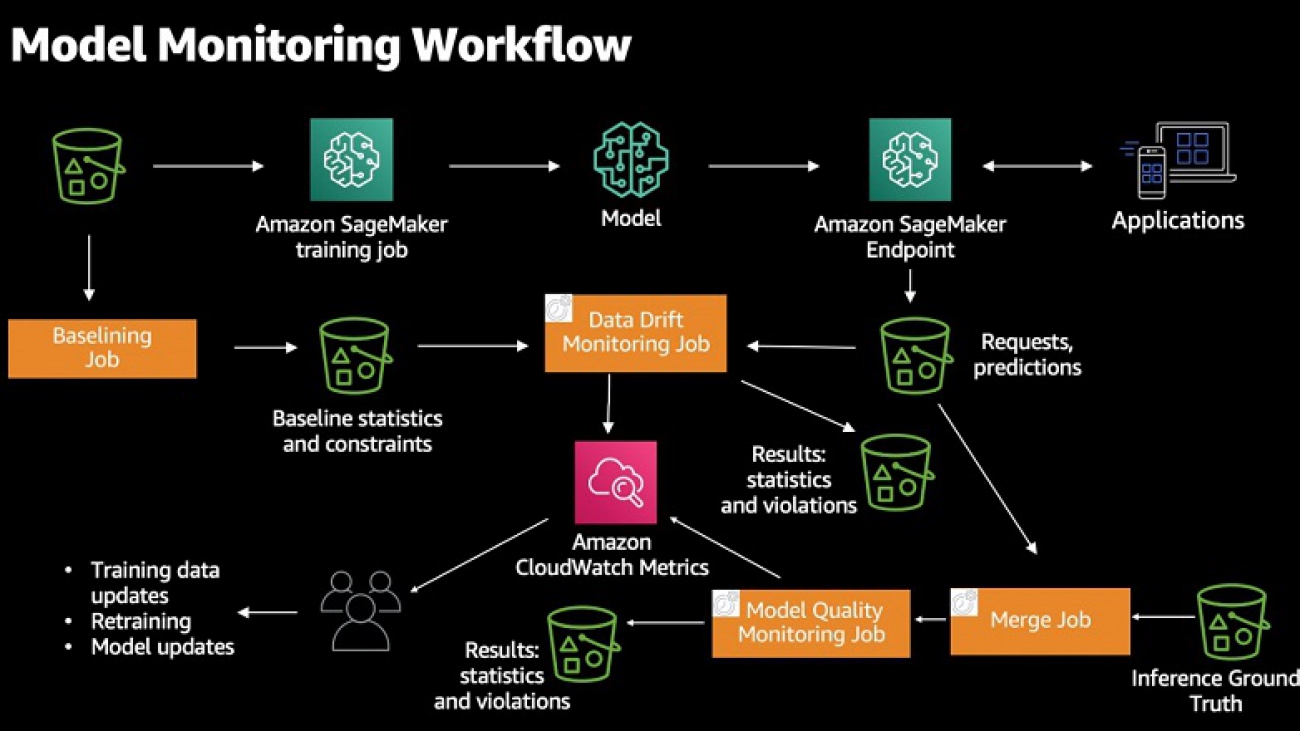
The following diagram illustrates the high-level workflow of Model Monitor. You start with an endpoint to monitor and configure a fraction of inference data to be captured in real time and stored in an Amazon Simple Storage Service (Amazon S3) bucket of your choice. Model Monitor allows you to capture both input data sent to an endpoint and predictions made by the model. After that, you can create a baseline job to generate statistical rules and constraints that serve as the basis for your model analysis later. Then, you define monitoring job and attach it to an endpoint through a schedule.

Model Monitor starts monitoring jobs to analyze the model prediction data collected during a given period. For monitoring model performance characteristics such as accuracy or precision in real time, Model Monitor allows you to ingest the ground truth labels collected from your applications. Model Monitor automatically merges the ground truth information with prediction data to compute the model performance metrics.

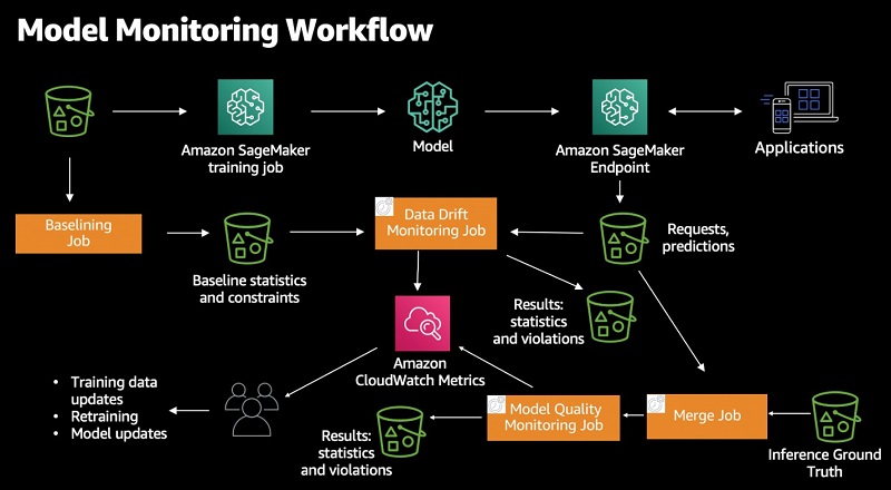
Model Monitor offers four different types of monitoring capabilities to detect and mitigate model drift in real time:

• Data quality – Helps detect change in statistical properties of independent variables and alerts you when a drift is detected.
• Model quality – Monitors model performance characteristics such as accuracy and precision in real time and alerts you when there is a degradation in model performance.
• Model bias – Helps you identify unwanted bias in your ML models and notify you when a bias is detected.
• Model explainability – Drift detection alerts you when there is a change in the relative importance of feature attributions.

For more information, see Amazon SageMaker Model Monitor.

The rest of this post dives into a notebook with the various steps involved in monitoring a pre-trained and deployed XGBoost customer churn binary classification model. You can use a similar approach for monitoring a regression model for increased error rates.

For detailed notebooks on other Model Monitor capabilities, see the data drift and bias notebook examples on GitHub.

Beyond the steps discussed in this post, there are other steps necessary to import libraries and set up AWS Identity and Access Management (IAM) permissions, and utility functions defined in the notebook, which this post doesn’t mention. You can walk through and run the code with the following notebook in the GitHub repo.

Monitoring model quality

To monitor our model quality, we complete two high-level steps:

• Deploy a pre-trained model with data capture enabled
• Generate a baseline for model quality performance

Deploying a pre-trained model

In this step, you deploy a pre-trained XGBoost churn prediction model to a SageMaker endpoint. The model was trained using the XGB Churn Prediction Notebook. If you have a pre-trained model that you want to monitor, you can use your own model in this step.

1. Upload a trained model artifact to an S3 bucket:

   s3_key = f"s3://{bucket}/{prefix}"
   model_url = S3Uploader.upload("model/xgb-churn-prediction-model.tar.gz", s3_key)
   model_url

You should see output similar to the following code:

s3://sagemaker-us-west-2-xxxxxxxxxxxx/sagemaker/DEMO-ModelMonitor-20200901/xgb-churn-prediction-model.tar.gz

2. Create a SageMaker model object:

   model_name = f"DEMO-xgb-churn-pred-model-monitor-{datetime.utcnow():%Y-%m-%d-%H%M}"
   image_uri = image_uris.retrieve(framework="xgboost", version="0.90-1", region=region)
   model = Model(image_uri=image_uri, model_data=model_url, role=role, sagemaker_session=session)

3. Create a variable to specify the data capture parameters. To enable data capture for monitoring the model data quality, you specify the capture option called DataCaptureConfig. You can capture the request payload, the response payload, or both with this configuration.

   endpoint_name = f"DEMO-xgb-churn-model-quality-monitor-{datetime.utcnow():%Y-%m-%d-%H%M}"
   print("EndpointName =", endpoint_name)
   
   data_capture_config = DataCaptureConfig(
                           enable_capture=True,
                           sampling_percentage=100,
                           destination_s3_uri=s3_capture_upload_path)
   
   model.deploy(initial_instance_count=1,
                instance_type='ml.m4.xlarge',
                endpoint_name=endpoint_name,
                data_capture_config=data_capture_config)

4. Create the SageMaker Predictor object from the endpoint to use for invoking the model:

   from sagemaker.predictor import Predictor
   
   predictor = Predictor(endpoint_name=endpoint_name, sagemaker_session=session, serializer=CSVSerializer())

Generating a baseline for model quality performance

In this step, you generate a baseline model quality that you can use to continuously monitor model quality against. To generate the model quality baseline, you first invoke the endpoint created earlier using validation data. Predictions from the deployed model using this validation data are used as a baseline dataset. You can use either the training or validation dataset to create the baseline. You then use Model Monitor to run a baseline job that computes model performance data and suggests model quality constraints based on the baseline dataset.

1. Invoke the endpoint with the following code:

   limit = 200 #Need at least 200 samples to compute standard deviations
   i = 0
   with open(f"test_data/{validate_dataset}", "w") as baseline_file:
       baseline_file.write("probability,prediction,labeln") # our header
       with open('test_data/validation.csv', 'r') as f:
           for row in f:
               (label, input_cols) = row.split(",", 1)
               probability = float(predictor.predict(input_cols))
               prediction = "1" if probability > churn_cutoff else "0"
               baseline_file.write(f"{probability},{prediction},{label}n")
               i += 1
               if i > limit:
                   break
               print(".", end="", flush=True)
               sleep(0.5)

2. Examine the predictions from the model:

   !head test_data/validation_with_predictions.csv

You see output similar to the following code:

probability,prediction,label
0.01516005303710699,0,0
0.1684480607509613,0,0
0.21427156031131744,0,0
0.06330718100070953,0,0
0.02791607193648815,0,0
0.014169521629810333,0,0
0.00571369007229805,0,0
0.10534518957138062,0,0
0.025899196043610573,0,0

Next, you configure a processing job to generate statistical rules and constraints (referred to as your baseline) against which the model quality drift can be detected. Model Monitor suggests a set of default baseline statistics and constraints. You can also bring in custom baseline constraints.

3. Start by uploading the validation data and predictions to Amazon S3:

   baseline_dataset_uri = S3Uploader.upload(f"test_data/{validate_dataset}", baseline_data_uri)
   baseline_dataset_uri

4. Create the model quality monitor:

   churn_model_quality_monitor = ModelQualityMonitor(
       role=role,
       instance_count=1,
       instance_type='ml.m5.xlarge',
       volume_size_in_gb=20,
       max_runtime_in_seconds=1800,
       sagemaker_session=session

5. Run the baseline suggestion processing job:

   job = churn_model_quality_monitor.suggest_baseline(
       job_name=baseline_job_name,
       baseline_dataset=baseline_dataset_uri,
       dataset_format=DatasetFormat.csv(header=True),
       output_s3_uri = baseline_results_uri,
       problem_type='BinaryClassification',
       inference_attribute= "prediction",
       probability_attribute= "probability",
       ground_truth_attribute= "label"
   )
   job.wait(logs=False)

When the baseline job is complete, you can explore the generated metrics and constraints.

6. View the binary classification metrics with the following code:

   binary_metrics = baseline_job.baseline_statistics().body_dict["binary_classification_metrics"]
   pd.json_normalize(baseline["binary_classification_metrics"]).T

The following screenshot shows your results.

7. View the constraints generated:

   constraints = json.loads(S3Downloader.read_file(constraints_file))
   constraints["binary_classification_constraints"]
   {'recall': {'threshold': 0.5714285714285714, 'comparison_operator': 'LessThanThreshold'},
    'precision': {'threshold': 1.0,             'comparison_operator': 'LessThanThreshold'},
    'accuracy': {'threshold': 0.9402985074626866,'comparison_operator': 'LessThanThreshold'),
    'true_positive_rate': {'threshold': 0.5714285714285714,'comparison_operator': 'LessThanThreshold'},
    'true_negative_rate': {'threshold': 1.0, 'comparison_operator': 'LessThanThreshold'},
    'false_positive_rate': {'threshold': 0.0,'comparison_operator': 'GreaterThanThreshold'),
    'false_negative_rate': {'threshold': 0.4285714285714286,'comparison_operator': 'GreaterThanThreshold'},
    'auc': {'threshold': 1.0, 'comparison_operator': 'LessThanThreshold'},
    'f0_5': {'threshold': 0.8695652173913042,'comparison_operator': 'LessThanThreshold'},
    'f1': {'threshold': 0.7272727272727273,'comparison_operator': 'LessThanThreshold'},
    'f2': {'threshold': 0.625, 'comparison_operator': 'LessThanThreshold'}}

From the constraints generated, you can see that model monitoring makes sure that the recall score from your model doesn’t regress and drop below 0.571. Similarly, it makes sure that you’re alerted when precision falls below 1.0. This may be too aggressive, but you can modify the generated constraints based on your use case and business needs.

Setting up continuous model monitoring

Now that you have the baseline of the model quality, you set up a continuous model monitoring job that monitors the quality of the deployed model against the baseline to identify model quality drift.

In addition to the generated baseline, Model Monitor needs two additional inputs: predictions made by the deployed model endpoint and the ground truth data to be provided by the model-consuming application. Because you already enabled data capture on the endpoint, prediction data is captured in Amazon S3. The ground truth data depends on the what your model is predicting and what the business use case is. In this case, because the model is predicting customer churn, ground truth data may indicate if the customer actually left the company or not. For the purposes of this notebook, you generate synthetic data as ground truth.

1. First generate traffic to the deployed endpoint. If there is no traffic, the monitoring jobs are marked as Failed because there is no data to process. See the following code:

   def invoke_endpoint(ep_name, file_name):    
       with open(file_name, 'r') as f:
           i = 0
           for row in f:
               payload = row.rstrip('n')
               response = session.sagemaker_runtime_client.invoke_endpoint(
                   EndpointName=endpoint_name,
                   ContentType='text/csv', 
                   Body=payload,
                   InferenceId=str(i), # unique ID per row
               )["Body"].read()
               i += 1
               sleep(1)
               
   def invoke_endpoint_forever():
       while True:
           invoke_endpoint(endpoint_name, 'test_data/test-dataset-input-cols.csv')
           
   thread = Thread(target = invoke_endpoint_forever)
   thread.start()

2. View the data captured with the following code:

   for _ in range(120):
       capture_files = sorted(S3Downloader.list(f"{s3_capture_upload_path}/{endpoint_name}"))
       if capture_files:
           capture_file = S3Downloader.read_file(capture_files[-1]).split("n")
           capture_record = json.loads(capture_file[0])
           if "inferenceId" in capture_record["eventMetadata"]:
               break
       print(".", end="", flush=True)
       sleep(1)
   print()
   print("Found Capture Files:")
   print("n ".join(capture_files[-5:]))

You see output similar to the following:

Found Capture Files:
s3://sagemaker-us-west-2-303008809627/sagemaker/Churn-ModelQualityMonitor-20201129/datacapture/DEMO-xgb-churn-model-quality-monitor-2020-12-01-2214/AllTraffic/2020/12/01/22/23-36-108-9df12912-2696-431e-a4ef-a76b3c3f7d32.jsonl
 s3://sagemaker-us-west-2-303008809627/sagemaker/Churn-ModelQualityMonitor-20201129/datacapture/DEMO-xgb-churn-model-quality-monitor-2020-12-01-2214/AllTraffic/2020/12/01/22/24-36-254-df884bcb-405c-4277-9cc8-517f3f31b56f.jsonl

3. View the contents of a single file:

   print(json.dumps(capture_record, indent=2))

You see output similar to the following:

{
  "captureData": {
    "endpointInput": {
      "observedContentType": "text/csv",
      "mode": "INPUT",
      "data": "75,0,109.0,88,259.3,120,182.1,119,13.3,3,4,0,0,0,0,0,0,0,0,0,0,0,0,0,0,0,0,0,0,0,0,0,0,0,0,0,0,0,0,0,0,0,0,0,0,0,0,0,0,1,0,0,0,0,0,0,0,0,0,0,0,0,0,0,1,1,0,1,0n",
      "encoding": "CSV"
    },
    "endpointOutput": {
      "observedContentType": "text/csv; charset=utf-8",
      "mode": "OUTPUT",
      "data": "0.7990730404853821",
      "encoding": "CSV"
    }
  },
  "eventMetadata": {
    "eventId": "01e27fce-a00a-4707-847e-9748d6a8e580",
    "inferenceTime": "2020-12-01T22:24:36Z"
  },
  "eventVersion": "0"
}

Next, you generate synthetic ground truth. Model Monitor allows you ingest the ground truth data collected periodically from your application and merge it with prediction data to compute model performance metrics. You can periodically upload the ground truth labels as they arrive and upload to Amazon S3. Model Monitor automatically merges the ground truth with prediction data and evaluates model performance against ground truth. The merged data is stored in Amazon S3 and can be accessed later for retraining your models. You can encrypt the data in this bucket and configure fine-grained security, access control mechanisms, and data retention policies.

4. Enter the following code to generate ground truth in the way that the SageMaker first party merge container expects:

   import random
   def ground_truth_with_id(inference_id):
       random.seed(inference_id) # to get consistent results
       rand = random.random()
       return {
           'groundTruthData': {
               'data': "1" if rand < 0.7 else "0", # randomly generate positive labels 70% of the time
               'encoding': 'CSV'
           },
           'eventMetadata': {
               'eventId': str(inference_id),
           },
           'eventVersion': '0',
       }
   def upload_ground_truth(records, upload_time):
       fake_records = [ json.dumps(r) for r in records ]
       data_to_upload = "n".join(fake_records)
       target_s3_uri = f"{ground_truth_upload_path}/{upload_time:%Y/%m/%d/%H/%M%S}.jsonl"
       print(f"Uploading {len(fake_records)} records to", target_s3_uri)
       S3Uploader.upload_string_as_file_body(data_to_upload, target_s3_uri)

The model quality job fails if either the data capture or ground truth data is missing.

Next, you set up a monitoring schedule that monitors the real-time performance of the model against the baseline.

5. Set the name of the monitoring scheduler:

   churn_monitor_schedule_name = 
   f"DEMO-xgb-churn-monitoring-schedule-{datetime.utcnow():%Y-%m-%d-%H%M}"
   

You now create the EndpointInput object. For the monitoring schedule, you need to specify how to interpret an endpoint’s output. Because the endpoint in this notebook outputs CSV data, the following code specifies that the first column of the output, 0, contains a probability (of churn in this example). You further specify 0.5 as the cutoff used to determine a positive label (that is, predict that a customer will churn).

6. Create the EndpointInput object with the following code:

   endpointInput = EndpointInput(endpoint_name=predictor.endpoint_name, 
                                 probability_attribute="0", 
                                 probability_threshold_attribute=0.8,
                                 destination='/opt/ml/processing/input_data')

7. Create the monitoring schedule. You specify how frequently the monitoring job runs using ScheduleExpression. In the following code, we set the schedule to one time per hour. For MonitoringType, you specify ModelQuality.

   response = churn_model_quality_monitor.create_monitoring_schedule(
       monitor_schedule_name=churn_monitor_schedule_name,
       endpoint_input=endpointInput,
       output_s3_uri = baseline_results_uri,
       problem_type='BinaryClassification',
       ground_truth_input=ground_truth_upload_path,
       constraints=baseline_job.suggested_constraints(),
       schedule_cron_expression=CronExpressionGenerator.hourly(), 
       enable_cloudwatch_metrics=True
         )

Each time the model quality monitoring job runs, it first runs a merge job and then a monitoring job. The merge job combines two different datasets: inference data collected by data capture enabled on the endpoint and ground truth inference data provided by you.

8. Examine a single run of the scheduled monitoring job:

   executions = churn_model_quality_monitor.list_executions()
   latest_execution = executions[-1]
   latest_execution.describe()
   status = execution['MonitoringExecutionStatus']
   
   while status in ["Pending", "InProgress"]:
       print("Waiting for execution to finish", end="")
       latest_execution.wait(logs=False)
       latest_job = latest_execution.describe()
       print()
       print(f"{latest_job['ProcessingJobName']} job status:", latest_job['ProcessingJobStatus'])
       print(f"{latest_job['ProcessingJobName']} job exit message, if any:", latest_job.get('ExitMessage'))
       print(f"{latest_job['ProcessingJobName']} job failure reason, if any:", latest_job.get('FailureReason'))
       sleep(30) # model quality executions consist of two Processing jobs, wait for second job to start
       latest_execution = churn_model_quality_monitor.list_executions()[-1]
       execution = churn_model_quality_monitor.describe_schedule()["LastMonitoringExecutionSummary"]
       status = execution['MonitoringExecutionStatus']
   
   print("Execution status is:", status)
       
   if status != 'Completed':
       print(execution)
       print("====STOP==== n No completed executions to inspect further. Please wait till an execution completes or investigate previously reported failures."

9. Check the violations against the baseline constraints:

   pd.options.display.max_colwidth = None
   violations = latest_execution.constraint_violations().body_dict["violations"]
   violations_df = pd.json_normalize(violations)
   violations_df.head(10)

The following screenshot shows the various violations generated.

From this list, you can see the false positive rate and false negative rate are both greater than the constraints generated or modified during the baselining step. Similarly, the accuracy and precision metrics are less than expected, indicating model quality degradation.

Analyzing model quality with Amazon CloudWatch metrics

In addition to the violations, the monitoring schedule also emits Amazon CloudWatch metrics. In this step, you view the metrics generated and set up a CloudWatch alarm to trigger when the model quality drifts from the baseline thresholds. You can also use CloudWatch alarms to trigger remedial actions such as retraining your model or updating the training dataset.

1. To view the list of the CloudWatch metrics generated, enter the following code:

   cw_client = boto3.Session().client('cloudwatch')
   namespace='aws/sagemaker/Endpoints/model-metrics'
   cw_dimenstions=[
           {
               'Name': 'Endpoint',
               'Value': endpoint_name
           },
           {
               'Name': 'MonitoringSchedule',
               'Value': churn_monitor_schedule_name
           }
   ]
   
   paginator = cw_client.get_paginator('list_metrics')
   for response in paginator.paginate(Dimensions=cw_dimenstions,Namespace=namespace):
       model_quality_metrics = response['Metrics']
       
       for metric in model_quality_metrics:
           print(metric['MetricName'])

You see output similar to the following:

f0_5_best_constant_classifier
f2_best_constant_classifier
f1_best_constant_classifier
auc
precision
accuracy_best_constant_classifier
true_positive_rate
f1
accuracy
false_positive_rate
f0_5
true_negative_rate
false_negative_rate
recall_best_constant_classifier
precision_best_constant_classifier
recall
f2

2. Create an alarm for when a specific metric doesn’t meet the threshold configured. In the following code, we create an alarm if the F2 value of the model falls below the threshold suggested by the baseline constraints:

   alarm_name='MODEL_QUALITY_F2_SCORE'
   alarm_desc='Trigger an cloudwatch alarm when the f2 score drifts away from the baseline constraints'
   mdoel_quality_f2_drift_threshold=0.625 ##Setting this threshold purposefully slow to see the alarm quickly.
   metric_name='f2'
   namespace='aws/sagemaker/Endpoints/model-metrics'
   
   #endpoint_name=endpoint_name
   #monitoring_schedule_name=mon_schedule_name
   
   cw_client.put_metric_alarm(
       AlarmName=alarm_name,
       AlarmDescription=alarm_desc,
       ActionsEnabled=True,
      #AlarmActions=[sns_notifications_topic],
       MetricName=metric_name,
       Namespace=namespace,
       Statistic='Average',
       Dimensions=[
           {
               'Name': 'Endpoint',
               'Value': endpoint_name
           },
           {
               'Name': 'MonitoringSchedule',
               'Value': churn_monitor_schedule_name
           }
       ],
       Period=600,
       EvaluationPeriods=1,
       DatapointsToAlarm=1,
       Threshold=mdoel_quality_f2_drift_threshold,
       ComparisonOperator='LessThanOrEqualToThreshold',
       TreatMissingData='breaching'
   )

In a few minutes, you should see a CloudWatch alarm created. The alarm first shows the status Insufficient Data and then changes to Alert. You can view its status on the CloudWatch console.

After you generate the alarm, you can decide on what actions you want to take on these alerts. A possible action could be updating the training data and retraining the model.

Visualizing the reports in Amazon SageMaker Studio

You can collect all the metrics that Model Monitor emits and view them in Amazon SageMaker Studio, a visual, fully integrated development environment (IDE) for ML so you can visually analyze your model performance without writing code or using third-party tools. You can also run ad-hoc analysis on the reports generated in a SageMaker notebook instance.

The following figure shows sample metrics and charts in Studio. Run the notebook in the Studio environment to view all metrics and charts related to the customer churn example.

Conclusion

SageMaker Model Monitoring is a very powerful tool that enables organizations employing ML models to create a continuous monitoring and model update cycle. This post discusses the monitoring capability with a focus on monitoring the quality of a deployed ML model. The notebook included with the post provides detailed instructions on monitoring an XGBoost binary classification model, along with a view into the baseline constraints generated and violations against the baseline constraints, and configures automated responses to the violations using CloudWatch alerts. This end-to-end workflow enables you to build continuous model training, monitoring, and model update pipelines. Give Model Monitor a try and leave your feedback in the comments.

About the Authors

Sireesha Muppala is an AI/ML Specialist Solutions Architect at AWS, providing guidance to customers on architecting and implementing machine learning solutions at scale. She received her Ph.D. in Computer Science from University of Colorado, Colorado Springs. In her spare time, Sireesha loves to run and hike Colorado trails.

David Nigenda is a Software Development Engineer in the Amazon SageMaker team. His current work focuses on providing useful insights on production machine learning workflows. In his spare time he tries to keep up with his kids.

Archana Padmasenan is a Senior Product Manager at Amazon SageMaker. She enjoys building products that delight customers.

Read More

Unity is one of the most popular game engines that has been adopted not only for video game development but also by industries such as film and automotive. Unity offers tools to create virtual simulated environments with customizable physics, landscapes, and characters. The Unity Machine Learning Agents Toolkit (ML-Agents) is an open-source project that enables developers to train reinforcement learning (RL) agents against the environments created on Unity.

Reinforcement learning is an area of machine learning (ML) that teaches a software agent how to take actions in an environment in order to maximize a long-term objective. For more information, see Amazon SageMaker RL – Managed Reinforcement Learning with Amazon SageMaker. ML-Agents is becoming an increasingly popular tool among many gaming companies for use cases such as game level difficulty design, bug fixing, and cheat detection. Currently, ML-Agents is used to train agents locally, and can’t scale to efficiently use more computing resources. You have to train RL agents on a local Unity engine for an extensive amount of time before obtaining the trained model. The process is time-consuming and not scalable for processing large amounts of data.

In this post, we demonstrate a solution by integrating the ML-Agents Unity interface with Amazon SageMaker RL, allowing you to train RL agents on Amazon SageMaker in a fully managed and scalable fashion.

Overview of solution

SageMaker is a fully managed service that enables fast model development. It provides many built-in features to assist you with training, tuning, debugging, and model deployment. SageMaker RL builds on top of SageMaker, adding pre-built RL libraries and making it easy to integrate with different simulation environments. You can use built-in deep learning frameworks such as TensorFlow and PyTorch with various built-in RL algorithms from the RLlib library to train RL policies. Infrastructures for training and inference are fully managed by SageMaker, so you can focus on RL formulation. SageMaker RL also provides a set of Jupyter notebooks, demonstrating varieties of domain RL applications in robotics, operations research, finance, and more.

The following diagram illustrates our solution architecture.

In this post, we walk through the specifics of training an RL agent on SageMaker by interacting with the sample Unity environment. To access the complete notebook for this post, see the SageMaker notebook example on GitHub.

Setting up your environments

To get started, we import the needed Python libraries and set up environments for permissions and configurations. The following code contains the steps to set up an Amazon Simple Storage Service (Amazon S3) bucket, define the training job prefix, specify the training job location, and create an AWS Identity and Access Management (IAM) role:

import sagemaker
import boto3
 
# set up the linkage and authentication to the S3 bucket
sage_session = sagemaker.session.Session()
s3_bucket = sage_session.default_bucket()  
s3_output_path = 's3://{}/'.format(s3_bucket)
print("S3 bucket path: {}".format(s3_output_path))

# create a descriptive job name
job_name_prefix = 'rl-unity-ray'

# configure where training happens – local or SageMaker instance
local_mode = False

if local_mode:
    instance_type = 'local'
else:
    # If on SageMaker, pick the instance type
    instance_type = "ml.c5.2xlarge"

# create an IAM role
try:
    role = sagemaker.get_execution_role()
except:
    role = get_execution_role()

print("Using IAM role arn: {}".format(role))

Building a Docker container

SageMaker uses Docker containers to run scripts, train algorithms, and deploy models. A Docker container is a standalone package of software that manages all the code and dependencies, and it includes everything needed to run an application. We start by building on top of a pre-built SageMaker Docker image that contains dependencies for Ray, then install the required core packages:

• gym-unity – Unity provides a wrapper to wrap Unity environment into a gym interface, an open-source library that gives you access to a set of classic RL environments
• mlagents-envs – Package that provides a Python API to allow direct interaction with the Unity game engine

Depending on the status of the machine, the Docker building process may take up to 10 minutes. For all pre-built SageMaker RL Docker images, see the GitHub repo.

Unity environment example

In this post, we use a simple example Unity environment called Basic. In the following visualization, the agent we’re controlling is the blue box that moves left or right. For each step it takes, it costs the agent some energy, incurring small negative rewards (-0.01). Green balls are targets with fixed locations. The agent is randomly initialized between the green balls, and collects rewards when it collides with the green balls. The large green ball offers a reward of +1, and the small green ball offers a reward of +0.1. The goal of this task is to train the agent to move towards the ball that offers the most cumulative rewards.

Model training, evaluation, and deployment

In this section, we walk you through the steps to train, evaluate, and deploy models.

Writing a training script

Before launching the SageMaker RL training job, we need to specify the configurations of the training process. It’s usually achieved in a single script outside the notebook. The training script defines the input (the Unity environment) and the algorithm for RL training. The following code shows what the script looks like:

import json
import os

import gym
import ray
from ray.tune import run_experiments
from ray.tune.registry import register_env

from sagemaker_rl.ray_launcher import SageMakerRayLauncher
from mlagents_envs.environment import UnityEnvironment
from mlagents_envs.exception import UnityWorkerInUseException
from mlagents_envs.registry import default_registry
from gym_unity.envs import UnityToGymWrapper

class UnityEnvWrapper(gym.Env):
    def __init__(self, env_config):
        self.worker_index = env_config.worker_index
        if 'SM_CHANNEL_TRAIN' in os.environ:
            env_name = os.environ['SM_CHANNEL_TRAIN'] +'/'+ env_config['env_name']
            os.chmod(env_name, 0o755)
            print("Changed environment binary into executable mode.")
            # Try connecting to the Unity3D game instance.
            while True:
                try:
                    unity_env = UnityEnvironment(
                                    env_name, 
                                    no_graphics=True, 
                                    worker_id=self.worker_index, 
                                    additional_args=['-logFile', 'unity.log'])
                except UnityWorkerInUseException:
                    self.worker_index += 1
                else:
                    break
        else:
            env_name = env_config['env_name']
            while True:
                try:
                    unity_env = default_registry[env_name].make(
                        no_graphics=True,
                        worker_id=self.worker_index,
                        additional_args=['-logFile', 'unity.log'])
                except UnityWorkerInUseException:
                    self.worker_index += 1
                else:
                    break
            
        self.env = UnityToGymWrapper(unity_env) 
        self.action_space = self.env.action_space
        self.observation_space = self.env.observation_space

    def reset(self):
        return self.env.reset()

    def step(self, action):
        return self.env.step(action)

class MyLauncher(SageMakerRayLauncher):

    def register_env_creator(self):
        register_env("unity_env", lambda config: UnityEnvWrapper(config))

    def get_experiment_config(self):
        return {
          "training": {
            "run": "PPO",
            "stop": {
              "timesteps_total": 10000,
            },
            "config": {
              "env": "unity_env",
              "gamma": 0.995,
              "kl_coeff": 1.0,
              "num_sgd_iter": 20,
              "lr": 0.0001,
              "sgd_minibatch_size": 100,
              "train_batch_size": 500,
              "monitor": True,  # Record videos.
              "model": {
                "free_log_std": True
              },
              "env_config":{
                "env_name": "Basic"
              },
              "num_workers": (self.num_cpus-1),
              "ignore_worker_failures": True,
            }
          }
        }

if __name__ == "__main__":
    MyLauncher().train_main()

The training script has two components:

• UnityEnvWrapper – The Unity environment is stored as a binary file. To load the environment, we need to use the Unity ML-Agents Python API. UnityEnvironment takes the name of the environment and returns an interactive environment object. We then wrap the object with UnityToGymWrapper and return an object that is trainable using Ray-RLLib and SageMaker RL.
• MyLauncher – This class inherits the SageMakerRayLauncher base class for SageMaker RL applications to use Ray-RLLib. Inside the class, we register the environment to be recognized by Ray and specify the configurations we want during training. Example hyperparameters include the name of the environment, discount factor in cumulative rewards, learning rate of the model, and number of iterations to run the model. For a full list of commonly used hyperparameters, see Common Parameters.

Training the model

After setting up the configuration and model customization, we’re ready to start the SageMaker RL training job. See the following code:

metric_definitions = RLEstimator.default_metric_definitions(RLToolkit.RAY)
    
estimator = RLEstimator(entry_point="train-unity.py",
                        source_dir='src',
                        dependencies=["common/sagemaker_rl"],
                        image_name=custom_image_name,
                        role=role,
                        train_instance_type=instance_type,
                        train_instance_count=1,
                        output_path=s3_output_path,
                        base_job_name=job_name_prefix,
                        metric_definitions=metric_definitions,
                        hyperparameters={
				# customize Ray parameters here
                        }
                    )

estimator.fit(wait=local_mode)
job_name = estimator.latest_training_job.job_name
print("Training job: %s" % job_name)

Inside the code, we specify a few parameters:

• entry_point – The path to the training script we wrote that specifies the training process
• source_dir – The path to the directory with other training source code dependencies aside from the entry point file
• dependencies – A list of paths to directories with additional libraries to be exported to the container

In addition, we state the container image name, training instance information, output path, and selected metrics. We are also allowed to customize any Ray-related parameters using the hyperparameters argument. We launch the SageMaker RL training job by calling estimator.fit, and start the model training process based on the specifications in the training script.

At a high level, the training job initiates a neural network and updates the network gradually towards the direction in which the agent collects higher reward. Through multiple trials, the agent eventually learns how to navigate to the high-rewarding location efficiently. SageMaker RL handles the entire process and allows you to view the training job status in the Training jobs page on the SageMaker console.

It’s also possible to monitor model performance by examining the training logs recorded in Amazon CloudWatch. Due to the simplicity of the task, the model completes training (10,000 agent movements) with roughly 800 episodes (number of times the agent reaches a target ball) in under 1 minute. The following plot shows the average reward collected converges around 0.9. The maximum reward the agent can get from this environment is 1, and each step costs 0.01, so a mean reward around 0.9 seems to be the results of optimal policy, indicating our training process is successful!

Evaluating the model

When model training is complete, we can load the trained model to evaluate its performance. Similar to the setup in the training script, we wrap the Unity environment with a gym wrapper. We then create an agent by loading the trained model.

To evaluate the model, we run the trained agent multiple times against the environment with a fixed agent and target initializations, and add up the cumulative rewards the agent collects at each step for each episode.

Out of five episodes, the average episode reward is 0.92 with the maximum reward of 0.93 and minimum reward of 0.89, suggesting the trained model indeed performs well.

Deploying the model

We can deploy the trained RL policy with just a few lines of code using the SageMaker model deployment API. You can pass an input and get out the optimal actions based on the policy. The input shape needs to match the observation input shape from the environment.

For the Basic environment, we deploy the model and pass an input to the predictor:

from sagemaker.tensorflow.model import TensorFlowModel

model = TensorFlowModel(model_data=estimator.model_data,
              framework_version='2.1.0',
              role=role)

predictor = model.deploy(initial_instance_count=1, 
                         instance_type=instance_type)

input = {"inputs": {'observations': np.ones(shape=(1, 20)).tolist(),
                    'prev_action': [0, 0],
                    'is_training': False,
                    'prev_reward': -1,
                    'seq_lens': -1
                   }
        }    

result = predictor.predict(input)
print(result['outputs']['actions'])

The model predicts an indicator corresponding to moving left or right. The recommended direction of movement for the blue box agent always points towards the larger green ball.

Cleaning up

When you’re finished running the model, call predictor.delete_endpoint() to delete the model deployment endpoint to avoid incurring future charges.

Customizing training algorithms, models, and environments

In addition to the preceding use case, we encourage you to explore the customization capabilities this solution supports.

In the preceding code example, we specify Proximal Policy Optimization (PPO) to be the training algorithm. PPO is a popular RL algorithm that performs comparably to state-of-the-art approaches but is much simpler to implement and tune. Depending on your use case, you can choose the most-fitted algorithm for training by either selecting from a list of comprehensive algorithms already implemented in RLLib or building a custom algorithm from scratch.

By default, RLLib applies a pre-defined convolutional neural network or fully connected neural network. However, you can create a custom model for training and testing. Following the examples from RLLib, you can register the custom model by calling ModelCatalog.register_custom_model, then refer to the newly registered model using the custom_model argument.

In our code example, we invoke a predefined Unity environment called Basic, but you can experiment with other pre-built Unity environments. However, as of this writing, our solution only supports a single-agent environment. When new environments are built, register it by calling register_env and refer to the environment with the env parameter.

Conclusion

In this post, we walk through how to train an RL agent to interact with Unity game environments using SageMaker RL. We use a pre-built Unity environment example for the demonstration, but encourage you to explore using custom or other pre-built Unity environments.

SageMaker RL offers a scalable and efficient way of training RL gaming agents to play game environments powered by Unity. For the notebook containing the complete code, see Unity 3D Game with Amazon SageMaker RL.

If you’d like help accelerating your use of ML in your products and processes, please contact the Amazon ML Solutions Lab.

About the Authors

Yohei Nakayama is a Deep Learning Architect at Amazon Machine Learning Solutions Lab, where he works with customers across different verticals to accelerate their use of artificial intelligence and AWS Cloud services to solve their business challenges. He is interested in applying ML/AI technologies to the space industry.

Henry Wang is a Data Scientist at Amazon Machine Learning Solutions Lab. Prior to joining AWS, he was a graduate student at Harvard in Computational Science and Engineering, where he worked on healthcare research with reinforcement learning. In his spare time, he enjoys playing tennis and golf, reading, and watching StarCraft II tournaments.

Yijie Zhuang is a Software Engineer with Amazon SageMaker. He did his MS in Computer Engineering from Duke. His interests lie in building scalable algorithms and reinforcement learning systems. He contributed to Amazon SageMaker built-in algorithms and Amazon SageMaker RL.

Read More