Amazon SageMaker Studio is a web-based fully integrated development environment (IDE) where you can perform end-to-end machine learning (ML) development to prepare data and build, train, and deploy models.

Like other AWS services, Studio supports a rich set of security-related features that allow you to build highly secure and compliant environments.

One of these fundamental security features allows you to launch Studio in your own Amazon Virtual Private Cloud (Amazon VPC). This allows you to control, monitor, and inspect network traffic within and outside your VPC using standard AWS networking and security capabilities. For more information, see Securing Amazon SageMaker Studio connectivity using a private VPC.

Customers in regulated industries, such as financial services, often don’t allow any internet access in ML environments. They often use only VPC endpoints for AWS services, and connect only to private source code repositories in which all libraries have been vetted both in terms of security and licensing. Customers may want to provide internet access but also have some controls such as domain name or URL filtering and allow access to only specific public repositories and websites, possibly packet inspection, or other network traffic-related security controls. For these cases, AWS Network Firewall and NAT gateway-based deployment may provide a suitable use case.

In this post, we show how you can use Network Firewall to build a secure and compliant environment by restricting and monitoring internet access, inspecting traffic, and using stateless and stateful firewall engine rules to control the network flow between Studio notebooks and the internet.

Depending on your security, compliance, and governance rules, you may not need to or cannot completely block internet access from Studio and your AI and ML workloads. You may have requirements beyond the scope of network security controls implemented by security groups and network access control lists (ACLs), such as application protocol protection, deep packet inspection, domain name filtering, and intrusion prevention system (IPS). Your network traffic controls may also require many more rules compared to what is currently supported in security groups and network ACLs. In these scenarios, you can use Network Firewall—a managed network firewall and IPS for your VPC.

Solution overview

When you deploy Studio in your VPC, you control how Studio accesses the internet with the parameter AppNetworkAccessType (via the Amazon SageMaker API) or by selecting your preference on the console when you create a Studio domain.

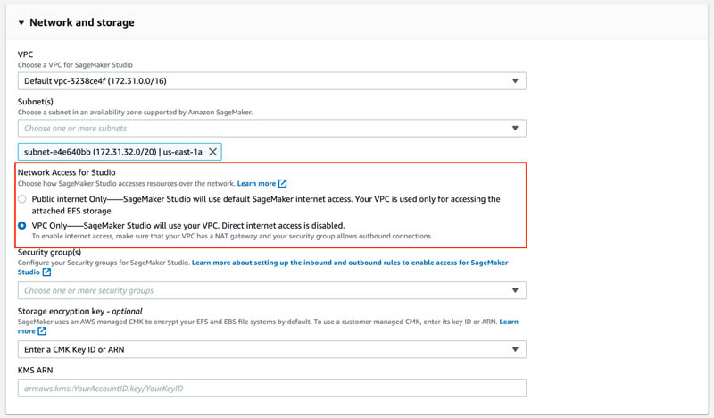
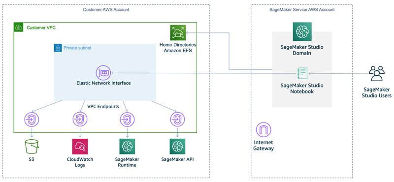
If you select Public internet Only (PublicInternetOnly), all the ingress and egress internet traffic from Amazon SageMaker notebooks flows through an AWS managed internet gateway attached to a VPC in your SageMaker account. The following diagram shows this network configuration.

Studio provides public internet egress through a platform-managed VPC for data scientists to download notebooks, packages, and datasets. Traffic to the attached Amazon Elastic File System (Amazon EFS) volume always goes through the customer VPC and never through the public internet egress.

To use your own control flow for the internet traffic, like a NAT or internet gateway, you must set the AppNetworkAccessType parameter to VpcOnly (or select VPC Only on the console). When you launch your app, this creates an elastic network interface in the specified subnets in your VPC. You can apply all available layers of security control—security groups, network ACLs, VPC endpoints, AWS PrivateLink, or Network Firewall endpoints—to the internal network and internet traffic to exercise fine-grained control of network access in Studio. The following diagram shows the VpcOnly network configuration.

In this mode, the direct internet access to or from notebooks is completely disabled, and all traffic is routed through an elastic network interface in your private VPC. This also includes traffic from Studio UI widgets and interfaces, such as Experiments, Autopilot, and Model Monitor, to their respective backend SageMaker APIs.

For more information about network access parameters when creating a domain, see CreateDomain.

The solution in this post uses the VpcOnly option and deploys the Studio domain into a VPC with three subnets:

• SageMaker subnet – Hosts all Studio workloads. All ingress and egress network flow is controlled by a security group.
• NAT subnet – Contains a NAT gateway. We use the NAT gateway to access the internet without exposing any private IP addresses from our private network.
• Network Firewall subnet – Contains a Network Firewall endpoint. The route tables are configured so that all inbound and outbound external network traffic is routed via Network Firewall. You can configure stateful and stateless Network Firewall policies to inspect, monitor, and control the traffic.

The following diagram shows the overview of the solution architecture and the deployed components.

VPC resources

The solution deploys the following resources in your account:

• A VPC with a specified Classless Inter-Domain Routing (CIDR) block
• Three private subnets with specified CIDRs
• Internet gateway, NAT gateway, Network Firewall, and a Network Firewall endpoint in the Network Firewall subnet
• A Network Firewall policy and stateful domain list group with an allow domain list
• Elastic IP allocated to the NAT gateway
• Two security groups for SageMaker workloads and VPC endpoints, respectively
• Four route tables with configured routes
• An Amazon S3 VPC endpoint (type Gateway)
• AWS service access VPC endpoints (type Interface) for various AWS services that need to be accessed from Studio

The solution also creates an AWS Identity and Access Management (IAM) execution role for SageMaker notebooks and Studio with preconfigured IAM policies.

Network routing for targets outside the VPC is configured in such a way that all ingress and egress internet traffic goes via the Network Firewall and NAT gateway. For details and reference network architectures with Network Firewall and NAT gateway, see Architecture with an internet gateway and a NAT gateway, Deployment models for AWS Network Firewall, and Enforce your AWS Network Firewall protections at scale with AWS Firewall Manager. The AWS re:Invent 2020 video Which inspection architecture is right for you? discusses which inspection architecture is right for your use case.

SageMaker resources

The solution creates a SageMaker domain and user profile.

The solution uses only one Availability Zone and is not highly available. A best practice is to use a Multi-AZ configuration for any production deployment. You can implement the highly available solution by duplicating the Single-AZ setup—subnets, NAT gateway, and Network Firewall endpoints—to additional Availability Zones.

You use Network Firewall and its policies to control entry and exit of the internet traffic in your VPC. You create an allow domain list rule to allow internet access to the specified network domains only and block traffic to any domain not on the allow list.

AWS CloudFormation resources

The source code and AWS CloudFormation template for solution deployment are provided in the GitHub repository. To deploy the solution on your account, you need:

• An AWS account and the AWS Command Line Interface (AWS CLI) configured with administrator permissions
• An Amazon Simple Storage Service (Amazon S3) bucket in your account in the same Region where you deploy the solution

Network Firewall is a Regional service; for more information on Region availability, see the AWS Region Table.

Your CloudFormation stack doesn’t have any required parameters. You may want to change the DomainName or *CIDR parameters to avoid naming conflicts with the existing resources and your VPC CIDR allocations. Otherwise, use the following default values:

• ProjectName – sagemaker-studio-vpc-firewall
• DomainName – sagemaker-anfw-domain
• UserProfileName – anfw-user-profile
• VPCCIDR – 10.2.0.0/16
• FirewallSubnetCIDR – 10.2.1.0/24
• NATGatewaySubnetCIDR – 10.2.2.0/24
• SageMakerStudioSubnetCIDR – 10.2.3.0/24

Deploy the CloudFormation template

To start experimenting with the Network Firewall and stateful rules, you need first to deploy the provided CloudFormation template to your AWS account.

1. Clone the GitHub repository:

git clone https://github.com/aws-samples/amazon-sagemaker-studio-vpc-networkfirewall.git
cd amazon-sagemaker-studio-vpc-networkfirewall 

2. Create an S3 bucket in the Region where you deploy the solution:

aws s3 mb s3://<your s3 bucket name>

You can skip this step if you already have an S3 bucket.

3. Deploy the CloudFormation stack:

make deploy CFN_ARTEFACT_S3_BUCKET=<your s3 bucket name>

The deployment procedure packages the CloudFormation template and copies it to the S3 bucket your provided. Then the CloudFormation template is deployed from the S3 bucket to your AWS account.

The stack deploys all the needed resources like VPC, network devices, route tables, security groups, S3 buckets, IAM policies and roles, and VPC endpoints, and also creates a new Studio domain and user profile.

When the deployment is complete, you can see the full list of stack output values by running the following command in terminal:

aws cloudformation describe-stacks 
    --stack-name sagemaker-studio-demo 
    --output table 
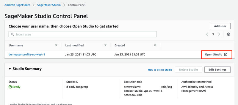
    --query "Stacks[0].Outputs[*].[OutputKey, OutputValue]"

4. Launch Studio via the SageMaker console.

Experiment with Network Firewall

Now you can learn how to control the internet inbound and outbound access with Network Firewall. In this section, we discuss the initial setup, accessing resources not on the allow list, adding domains to the allow list, configuring logging, and additional firewall rules.

Initial setup

The solution deploys a Network Firewall policy with a stateful rule group with an allow domain list. This policy is attached to the Network Firewall. All inbound and outbound internet traffic is blocked now, except for the .kaggle.com domain, which is on the allow list.

Let’s try to access https://kaggle.com by opening a new notebook in Studio and attempting to download the front page from kaggle.com:

!wget https://kaggle.com

The following screenshot shows that the request succeeds because the domain is allowed by the firewall policy. Users can connect to this and only to this domain from any Studio notebook.

Access resources not on the allowed domain list

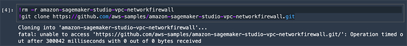
In the Studio notebook, try to clone any public GitHub repository, such as the following:

!git clone https://github.com/aws-samples/amazon-sagemaker-studio-vpc-networkfirewall.git

This operation times out after 5 minutes because any internet traffic except to and from the .kaggle.com domain isn’t allowed and is dropped by Network Firewall.

Add a domain to the allowed domain list

To be able to run the git clone command, you must allow internet traffic to the .github.com domain.

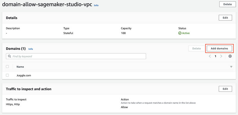
1. On the Amazon VPC console, choose Firewall policies.
2. Choose the policy network-firewall-policy-<ProjectName>.

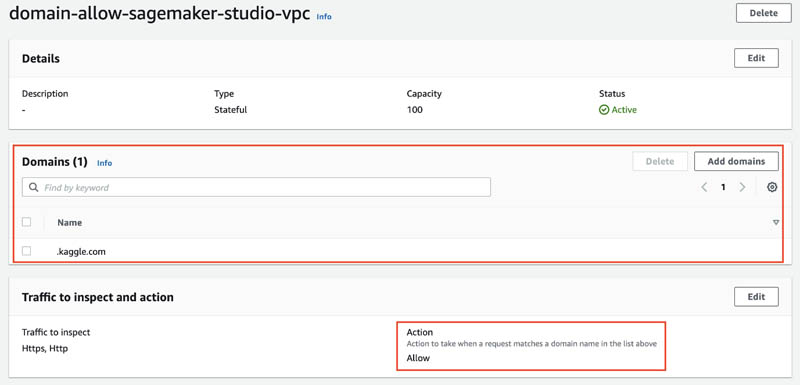
3. In the Stateful rule groups section, select the group rule domain-allow-sagemaker-<ProjectName>.

You can see the domain .kaggle.com on the allow list.

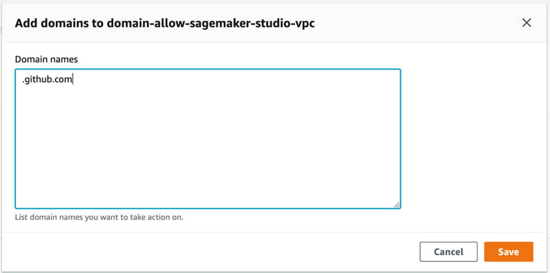
4. Choose Add domain.

5. Enter .github.com.
6. Choose Save.

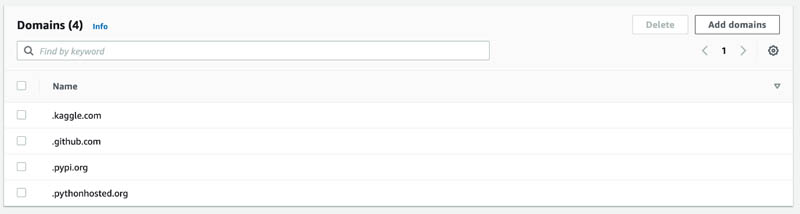
You now have two names on the allow domain list.

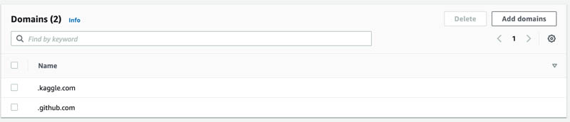
Firewall policy is propagated in real time to Network Firewall and your changes take effect immediately. Any inbound or outbound traffic from or to these domains is now allowed by the firewall and all other traffic is dropped.

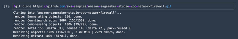
To validate the new configuration, go to your Studio notebook and try to clone the same GitHub repository again:

!git clone https://github.com/aws-samples/amazon-sagemaker-studio-vpc-networkfirewall.git

The operation succeeds this time—Network Firewall allows access to the .github.com domain.

Network Firewall logging

In this section, you configure Network Firewall logging for your firewall’s stateful engine. Logging gives you detailed information about network traffic, including the time that the stateful engine received a packet, detailed information about the packet, and any stateful rule action taken against the packet. The logs are published to the log destination that you configured, where you can retrieve and view them.

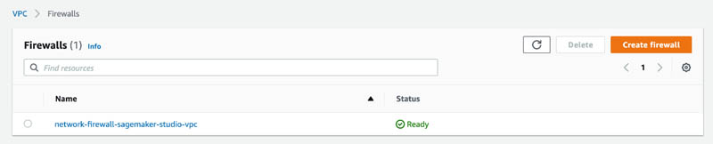
1. On the Amazon VPC console, choose Firewalls.
2. Choose your firewall.

3. Choose the Firewall details tab.

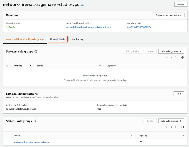
4. In the Logging section, choose Edit.

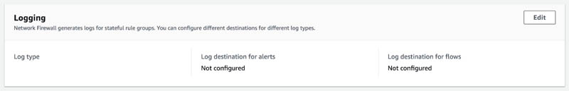
5. Configure your firewall logging by selecting what log types you want to capture and providing the log destination.

For this post, select Alert log type, set Log destination for alerts to CloudWatch Log group, and provide an existing or a new log group where the firewall logs are delivered.

6. Choose Save.

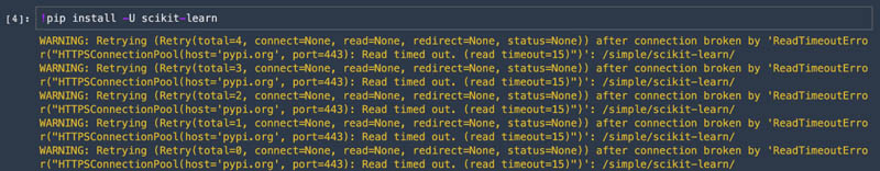
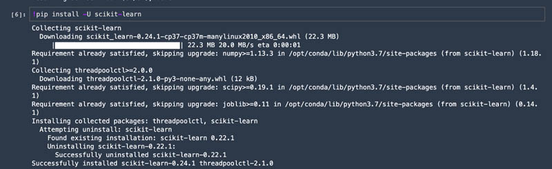
To check your settings, go back to Studio and try to access pypi.org to install a Python package:

!pip install -U scikit-learn

This command fails with ReadTimeoutError because Network Firewall drops any traffic to any domain not on the allow list (which contains only two domains: .github.com and .kaggle.com).

On the Amazon CloudWatch console, navigate to the log group and browse through the recent log streams.

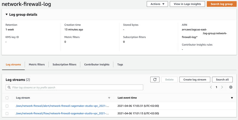
The pipy.org domain shows the blocked action. The log event also provides additional details such as various timestamps, protocol, port and IP details, event type, availability zone, and the firewall name.

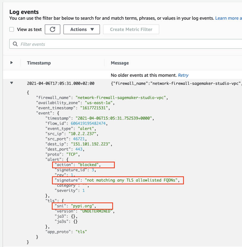
You can continue experimenting with Network Firewall by adding .pypi.org and .pythonhosted.org domains to the allowed domain list.

Then validate your access to them via your Studio notebook.

Additional firewall rules

You can create any other stateless or stateful firewall rules and implement traffic filtering based on a standard stateful 5-tuple rule for network traffic inspection (protocol, source IP, source port, destination IP, destination port). Network Firewall also supports industry standard stateful Suricata compatible IPS rule groups. You can implement protocol-based rules to detect and block any non-standard or promiscuous usage or activity. For more information about creating and managing Network Firewall rule groups, see Rule groups in AWS Network Firewall.

Additional security controls with Network Firewall

In the previous section, we looked at one feature of the Network Firewall: filtering network traffic based on the domain name. In addition to stateless or stateful firewall rules, Network Firewall provides several tools and features for further security controls and monitoring:

• Central firewall management and visibility in AWS Firewall Manager. You can centrally manage security policies and automatically enforce mandatory security policies across existing and newly created accounts and VPCs.
• Network Firewall logging for the firewall’s stateful engine. You can record flow and alert logs, and use the same or different logging destinations for each log type.
• Stateless rules to filter network traffic based on protocol, source IP addresses, ranges, source port ranges, destination IP addresses and ranges, and TCP flags.
• Integration into a broader set of AWS security components. For an example, see Automatically block suspicious traffic with AWS Network Firewall and Amazon GuardDuty.
• Integration in a diverse ecosystem of Network Firewall Partners that complement Network Firewall, enabling the deployment of a comprehensive security architecture. For example use cases, see Full VPC traffic visibility with AWS Network Firewall and Sumo Logic and Splunk Named Launch Partner of AWS Network Firewall.

Build secure ML environments

A robust security design normally includes multi-layer security controls for the system. For SageMaker environments and workloads, you can use the following AWS security services and concepts to secure, control, and monitor your environment:

• VPC and private subnets to perform secure API calls to other AWS services and restrict internet access for downloading packages.
• S3 bucket policies that restrict access to specific VPC endpoints.
• Encryption of ML model artifacts and other system artifacts that are either in transit or at rest. Requests to the SageMaker API and console are made over a Secure Sockets Layer (SSL) connection.
• Restricted IAM roles and policies for SageMaker runs and notebook access based on resource tags and project ID.
• Restricted access to Amazon public services, such as Amazon Elastic Container Registry (Amazon ECR) to VPC endpoints only.

For a reference deployment architecture and ready-to-use deployable constructs for your environment, see Amazon SageMaker with Guardrails on AWS.

Conclusion

In this post, we showed how you can secure, log, and monitor internet ingress and egress traffic in Studio notebooks for your sensitive ML workloads using managed Network Firewall. You can use the provided CloudFormation templates to automate SageMaker deployment as part of your Infrastructure as Code (IaC) strategy.

For more information about other possibilities to secure your SageMaker deployments and ML workloads, see Building secure machine learning environments with Amazon SageMaker.

About the Author

Yevgeniy Ilyin is a Solutions Architect at AWS. He has over 20 years of experience working at all levels of software development and solutions architecture and has used programming languages from COBOL and Assembler to .NET, Java, and Python. He develops and codes cloud native solutions with a focus on big data, analytics, and data engineering.

Read More

Medical providers often need to analyze and dictate patient phone conversations, doctors’ notes, clinical trial reports, and patient health records. By automating transcription, providers can quickly and accurately provide patients with medical conditions, medication, dosage, strength, and frequency.

Generic artificial intelligence-based transcription models can be used to transcribe voice to text. However, medical voice data often uses complex medical terms and abbreviations. Transcribing such data needs medical/healthcare-specific machine learning (ML) models. To address this issue, AWS launched Amazon Transcribe Medical, an automatic speech recognition (ASR) service that makes it easy for you to add medical speech-to-text capabilities to your voice-enabled applications.

Additionally, Amazon Comprehend Medical is a HIPAA-eligible service that helps providers extract information from unstructured medical text accurately and quickly. To transcribe voice in real time, providers need access to raw audio from the call while in-progress. Twilio, an AWS partner, offers real-time telephone voice integration.

In this post, we show you how to integrate Twilio Media Streams with Amazon Transcribe Medical and Amazon Comprehend Medical to transcribe and analyze data from phone calls. For non-healthcare industries, you can use this same solution with Amazon Transcribe and Amazon Comprehend.

Twilio Media Streams works in the context of a traditional Twilio voice application, like an Interactive Voice Response (IVR), that serves customers directly, as well as a contact center, like Twilio Flex, where agents are serving consumers. You have discrete control over your voice data within your contact center to build the experience your customers prefer.

Amazon Transcribe Medical is an ML service that makes it easy to quickly create accurate transcriptions between patients and physicians. Amazon Comprehend Medical is a natural language processing (NLP) service that makes it easy to use ML to extract relevant medical information from unstructured text. You can quickly and accurately gather information (such as medical condition, medication, dosage, strength, and frequency), from a variety of sources (like doctors’ notes, clinical trial reports, and patient health records). Amazon Comprehend Medical can also link the detected information to medical ontologies such as ICD-10-CM or RxNorm so downstream healthcare applications can use it easily.

The following diagram illustrates how Amazon Comprehend Medical supports medical named entity and relationship extractions.

Amazon Transcribe Medical, Amazon Comprehend Medical, and Twilio Media Streams are all managed platforms. This means that data scientists and healthcare IT teams don’t need to build services from the ground up. Voice integration is provided by Twilio and  AWS ML services APIs, and only requires a simple plug-and-play with AWS and Twilio services to build the end-to-end workflow.

Solution overview

Our solution uses Twilio Media Streams to provide telephony service to the customer. This service provides a telephone number and backend to media services to integrate it with REST API-based web applications. In this solution, we build a Node.js web app and deploy it with AWS Amplify. Amplify helps front-end web and mobile developers build secure, scalable, full stack applications. The web app interfaces with Twilio Media Streams to receive phone calls in voice format, and uses Amazon Transcribe Medical to convert voice to text. Upon receiving the transcription, the application interfaces with Amazon Comprehend Medical to extract medical terms and insights from the transcription. The insights are displayed on the web app and stored in an Amazon DynamoDB table for further analysis. The solution also uses Amazon Simple Storage Service (Amazon S3) and an AWS Cloud9 environment.

The following diagram illustrates the solution architecture.

To implement the solution, we complete the following high-level steps:

1. Create a trial Twilio account.
2. Create an AWS Identity and Access Management (IAM) user.
3. Create an AWS Cloud9 integrated development environment (IDE).
4. Clone the GitHub repo.
5. Create a secured HTTPS tunnel using ngrok and set up Twilio phone number’s voice configuration.
6. Run the application.

Create a trial Twilio account

Before getting started, make sure to sign up for a trial Twilio account (https://www.twilio.com/try-twilio), if you don’t already have one.

Create an IAM user

To create an IAM user, complete the following steps:

1. On the IAM console, under Access management, choose Users.
2. Choose Add user.
3. On the Set user details page, for User name¸ enter a name.
4. For Access type, select Programmatic access.
5. Choose Next: Permissions.

6. On the Set permissions page, choose Attach existing policies directly.
7. Select the following AWS Managed Policies, AmazonTranscribeFullAccess, ComprehendMedicalFullAccess, AmazonDyanmoDBFullAccess, and AmazonS3FullAccess.
8. Choose Next: Tags.
9. Skip adding tags and choose Next: Review.
10. Review the IAM user details and attached policies and choose Create user.

11. On the next page, copy the access key ID and secret access key to your clipboard or download the CSV file.

We use these credentials for testing the Node.js application.

Create an S3 Bucket

To create your Amazon S3 Bucket, complete the following steps.

1. On the Amazon S3 console, choose Create bucket.
2. For Bucket name, enter a name for the Amazon S3 bucket.
3. For Block Public Access settings for this bucket check Block all public access.
4. Review the settings and choose Create bucket.

Create an Amazon DynamoDB Table

To create your Amazon DynamoDB table, complete the following steps.

1. On the Amazon DynamoDB console, choose Create table.
2. For Table name, enter a name for the Amazon DynamoDB Table.
3. For Primary key, enter ROWID for the primary key.

4. Review the Amazon DynamoDB table settings and choose

Create an AWS Cloud9 environment

To create your AWS Cloud9 environment, complete the following steps.

1. On the AWS Cloud9 console, choose Environments.
2. Choose Create environment.
3. For Name, enter a name for the environment.
4. For Description, enter an optional description.
5. Choose Next step.

6. On the Configure Settings page, select Ubuntu Server 18.04 LTS for Platform and leave the other settings as default.

7. Review the settings and choose Create environment.

The AWS Cloud9 IDE tab opens on your browser; you may have to wait a few minutes for the environment creation process to complete.

Clone the GitHub repo

In the AWS Cloud9 environment, close the Welcome and AWS Toolkit – QuickStart tabs. To clone the GitHub repository, on the bash terminal, enter the following code:

git clone https://github.com/aws-samples/amazon-transcribe-comprehend-medical-twilio

cd twilio-medical-transcribe && npm install --silent

Edit the config.json file under the project directory. Replace the values with your Amazon S3 Bucket and Amazon DynamoDB table.

Set up ngrok and the Twilio phone number

Before we start the Node.js application, we need to start a secured HTTPS tunnel using ngrok and set up the Twilio phone number’s voice configuration.

1. On the terminal, choose the +
2. Choose New Terminal.

3. On the terminal, install ngrok:

   sudo snap install ngrok

4. After ngrok is installed, run the following code to expose the local Express Node.js server to the internet:

   ngrok http 8080

5. Copy the public HTTPS URL.

You use this URL for the Twilio phone number’s voice configuration.

6. Sign in to your Twilio account.
7. On the dashboard, choose the … icon to open the Settings

8. Choose Phone Numbers.

9. On the Phone Numbers page, choose your Twilio phone number.

10. In the Voice section, for A Call Comes In, choose Webhook.
11. Enter the ngrok tunnel followed by /twiml.
12. Save the configuration.

Run the application

Let’s now run the Twilio Media Streams, Amazon Transcribe Medical, and Amazon Comprehend Medical services by entering the following code:

npm start

We can preview the application in AWS Cloud9. In the environment, on the Preview menu, choose Preview Running Application.

You can copy the public URL to view the application in another browser tab.

Enter the IAM user access ID and secret key credentials, and your Twilio account SID, auth token, and phone number.

Demonstration

In this section, we use two sample recordings to demonstrate real-time audio transcription with Twilio Media Streams.

After you enter your IAM and Twilio credentials, choose Submit Credentials.

The following screenshot shows the transcription for our first audio file, sample-1.mp4.

The following screenshot shows the transcription for our second file, sample-3.mp4.

This application uses Amazon Transcribe Medical to transcribe media content in real time, and stores the output in Amazon S3 for further analysis. The application then uses Amazon Comprehend Medical to detect the following entities:

• ANATOMY – Detects references to the parts of the body or body systems and the locations of those parts or systems
• MEDICAL_CONDITION – Detects the signs, symptoms, and diagnosis of medical conditions
• MEDICATION – Detects medication and dosage information for the patient
• PROTECTED_HEALTH_INFORMATION – Detects the patient’s personal information
• TEST_TREATMENT_PROCEDURE – Detects the procedures that are used to determine a medical condition
• TIME_EXPRESSION – Detects entities related to time when they are associated with a detected entity

These entities are stored in the DynamoDB table. Healthcare providers can use this data to create patient diagnosis and treatment plan.

You can further analyze this data through services such as Amazon Elasticsearch Service (Amazon ES) and Amazon Kendra.

Clean up your resources

The AWS services used in this solution are part of the AWS Free Tier. If you’re not using the Free Tier, clean up the following resources to avoid incurring additional charges:

• AWS Cloud9 environment
• Amazon S3 Bucket
• Amazon DynamoDB Table
• IAM user

Conclusion

In this post, we showed how to integrate Twilio Media Streams with Amazon Transcribe Medical and Amazon Comprehend Medical to transcribe and analyze medical data from audio files. You can also use this solution in non-healthcare industries to transcribe information from audio.

We invite you to check out the code in the GitHub repo and try out the solution, and even expand on the data analysis with Amazon ES or Amazon Kendra.

About the Author

Mahendra Bairagi is a Principal Machine Learning Prototyping Architect at Amazon Web Services. He helps customers build machine learning solutions on AWS. He has extensive experience on ML, Robotics, IoT and Analytics services. Prior to joining Amazon Web Services, he had long tenure as entrepreneur, enterprise architect and software developer.

Jay Park is a Prototyping Solutions Architect for AWS. Jay is focused on helping AWS customers speed their adoption of cloud-native workloads through rapid prototyping

Read More

Amazon Forecast now displays the estimated time it takes to complete an in-progress workflow for importing your data, training the predictor, and generating the forecast. You can now manage your time more efficiently and better plan for your next workflow around the estimated time remaining for your in-progress workflow. Forecast uses machine learning (ML) to generate more accurate demand forecasts, without requiring any prior ML experience. Forecast brings the same technology used at Amazon.com to developers as a fully managed service, removing the need to manage resources or rebuild your systems.

Previously, you had no clear insights as to how long a workflow would take to complete, which forced you to proactively monitor each stage, whether it was importing your data, training the predictor, or generating the forecast. This made it difficult for you to plan for subsequent steps, causing frustration and anxiety. This can be especially frustrating when the time required to import data, train a predictor, and creating forecasts can vary widely depending on the size and characteristics of your data.

Now, you have visibility into the time that a workflow may take, which can be especially useful for manually running your forecast workloads and during the process of experimentation. Knowing how long each workflow will take allows you to focus on other tasks and come back to the forecast journey later. Additionally, the displayed estimated time to complete a workflow refreshes automatically, which provides better expectations and removes further frustration.

In this post, we walk through the Forecast console experience of reading the estimated time to workflow completion. To check the estimated time through the APIs, refer to DescribeDatasetImportJob, DescribePredictor, DescribeForecast.

If you want to build automated workflows for Forecast, we recommend following the steps outlined in Create forecasting systems faster with automated workflows and notifications in Amazon Forecast, which walks through integrating Forecast with Amazon EventBridge to build event-driven Forecast workflows. EventBridge removes the need to manually check the estimated time for a workflow to complete, because it starts your desired next workflow automatically.

Check the estimated time to completion of your dataset import workflow

After you create a new dataset import job, you can see the Create pending status for the newly created job. When the status changes to Create in progress, you can see the estimated time remaining in the Status column of the Datasets imports section. This estimated time refreshes automatically until the status changes to Active.

On the details page of the newly created dataset import job, when the status is Create in progress, the Estimated time remaining field shows the remaining time for the import job to complete and Actual import time shows -. This section refreshes automatically with the estimated time to completion. After the import job is complete and the status becomes Active, the Actual import time shows the total time of the import.

Check the estimated time to completion of your predictor training workflow

After you create a new predictor, you first see the Create pending status for the newly created job. When the status changes to Create in progress, you see the estimated time remaining in the Status column in the Predictors section. This estimated time refreshes automatically until the status changes to Active.

On the details page of the newly created predictor job, when the status is Create in progress, the Estimated time remaining field shows the remaining time for the predictor job to complete and Actual import time shows -. This section refreshes automatically with the estimated time to completion. After the import job is complete and the status becomes Active, the Actual import time shows the total time for the predictor creation.

Check the estimated time to completion of your forecast creation workflow

After you create a new forecast, you first see the Create pending status for the newly created job. When the status changes to Create in progress, you see the estimated time remaining in the Status column. This estimated time refreshes automatically until it changes to Active.

On the details page of the newly created forecast job, when the status is Create in progress, the Estimated time remaining field shows the remaining time for the forecast job to complete and Actual import time shows -. This section refreshes automatically with the estimated time to completion. After the import job is complete and the status changes to Active, the Actual import time shows the total time for the forecast creation to complete.

Conclusion

You can now find out how long it takes when you initiate a workload using Forecast, which can help you manage your time more efficiently. The new field is part of the response to Describe* calls that will show up automatically, without requiring any setup.

To learn more about this capability, see DescribeDatasetImportJob, DescribePredictor, and DescribeForecast. You can use this capability in all Regions where Forecast is publicly available. For more information about Region availability, see AWS Regional Services.

About the Authors

Alex Kim is a Sr. Product Manager for Amazon Forecast. His mission is to deliver AI/ML solutions to all customers who can benefit from it. In his free time, he enjoys all types of sports and discovering new places to eat.

Ranjith Kumar Bodla is an SDE in the Amazon Forecast team. He works as a backend developer within a distributed environment with a focus on AI/ML and leadership. During his spare time, he enjoys playing table tennis, traveling, and reading.

Gautam Puri is a Software Development Engineer on the Amazon Forecast team. His focus area is on building distributed systems that solve machine learning problems. In his free time, he enjoys hiking and basketball.

Shannon Killingsworth is a UX Designer for Amazon Forecast and Amazon Personalize. His current work is creating console experiences that are usable by anyone, and integrating new features into the console experience. In his spare time, he is a fitness and automobile enthusiast.

Read More

Amazon Lookout for Vision is a machine learning (ML) service that spots defects and anomalies in visual representations using computer vision (CV). With Amazon Lookout for Vision, manufacturing companies can increase quality and reduce operational costs by quickly identifying differences in images of objects at scale.

Many enterprise customers want to identify missing components in products, damage to vehicles or structures, irregularities in production lines, minuscule defects in silicon wafers, and other similar problems. Amazon Lookout for Vision uses ML to see and understand images from any camera as a person would, but with an even higher degree of accuracy and at a much larger scale. Amazon Lookout for Vision eliminates the need for costly and inconsistent manual inspection, while improving quality control, defect and damage assessment, and compliance. In minutes, you can begin using Amazon Lookout for Vision to automate inspection of images and objects—with no ML expertise required.

In this post, we look at how we can automate detecting anomalies in silicon wafers and notifying operators in real time.

Solution overview

Keeping track of the quality of products in a manufacturing line is a challenging task. Some process steps take images of the product that humans then review in order to assure good quality. Thanks to artificial intelligence, you can automate these anomaly detection tasks, but human intervention may be necessary after anomalies are detected. A standard approach is sending emails when problematic products are detected. These emails might be overlooked, which could cause a loss in quality in a manufacturing plant.

In this post, we automate the process of detecting anomalies in silicon wafers and notifying operators in real time using automated phone calls. The following diagram illustrates our architecture. We deploy a static website using AWS Amplify, which serves as the entry point for our application. Whenever a new image is uploaded via the UI (1), an AWS Lambda function invokes the Amazon Lookout for Vision model (2) and predicts whether this wafer is anomalous or not. The function stores each uploaded image to Amazon Simple Storage Service (Amazon S3) (3). If the wafer is anomalous, the function sends the confidence of the prediction to Amazon Connect and calls an operator (4), who can take further action (5).

Setting up Amazon Connect and the associated contact flow

To configure Amazon Connect and the contact flow, you complete the following high-level steps:

1. Create an Amazon Connect instance.
2. Set up the contact flow.
3. Claim your phone number.

Create an Amazon Connect instance

The first step is to create an Amazon Connect instance. For the rest of the setup, we use the default values, but don’t forget to create an administrator login.

Instance creation can take a few minutes, after which we can log in to the Amazon Connect instance using the admin account we created.

Setting up the contact flow

In this post, we have a predefined contact flow that we can import. For more information about importing an existing contact flow, see Import/export contact flows.

1. Choose the file contact-flow/wafer-anomaly-detection from the GitHub repo.
2. Choose Import.

The imported contact flow looks similar to the following screenshot.

3. On the flow details page, expand Show additional flow information.

Here you can find the ARN of the contact flow.

4. Record the contact flow ID and contact center ID, which you need later.

Claim your phone number

Claiming a number is easy and takes just a few clicks. Make sure to choose the previously imported contact flow while claiming the number.

If no numbers are available in the country of your choice, raise a support ticket.

Contact flow overview

The following screenshot shows our contact flow.

The contact flow performs the following functions:

• Enable logging
• Set the output Amazon Polly voice (for this post, we use the Kendra voice)
• Get customer input using DTMF (only keys 1 and 2 are valid).
• Based on the user’s input, the flow does one of the following:
  • Prompt a goodbye message stating no action will be taken and exit
  • Prompt a goodbye message stating an action will be taken and exit
  • Fail and deliver a fallback block stating that the machine will shut down and exit

Optionally, you can enhance your system with an Amazon Lex bot.

Deploy the solution

Now that you have set up Amazon Connect, deployed your contact flow, and noted the information you need for the rest of the deployment, we can deploy the remaining components. In the cloned GitHub repository, edit the build.sh script and run it from the command line:

#Global variables
ApplicationRegion="YOUR_REGION"
S3SourceBucket="YOUR_S3_BUCKET-sagemaker"
LookoutProjectName="YOUR_PROJECT_NAME"
FlowID="YOUR_FLOW_ID"
InstanceID="YOUR_INSTANCE_ID"
SourceNumber="YOUR_CLAIMED_NUMBER"
DestNumber="YOUR_MOBILE_PHONE_NUMBER"
CloudFormationStack="YOUR_CLOUD_FORMATION_STACK_NAME"

Provide the following information:

• Your Region
• The S3 bucket name you want to use (make sure the name includes the word sagemaker).
• The name of the Amazon Lookout for Vision project you want to use
• The ID of your contact flow
• Your Amazon Connect instance ID
• The number you’ve claimed in Amazon Connect in E.164 format (for example, +132398765)
• A name for the AWS CloudFormation stack you create by running this script

This script then performs the following actions:

• Create an S3 bucket for you
• Build the .zip files for your Lambda function
• Upload the CloudFormation template and the Lambda function to your new S3 bucket
• Create the CloudFormation stack

After the stack is deployed, you can find the following resources created on the AWS CloudFormation console.

You can see that an Amazon SageMaker notebook called amazon-lookout-vision-create-project is also created.

Build, train, and deploy the Amazon Lookout for Vision model

In this section, we see how to build, train, and deploy the Amazon Lookout for Vision model using the open-source Python SDK. For more information about the Amazon Lookout for Vision Python SDK, see this blog post.

You can build the model via the AWS Management Console. For programmatic deployment, complete the following steps:

1. On the SageMaker console, on the Notebook instances page, access the SageMaker notebook instance that was created earlier by choosing Open Jupyter.

In the instance, you can find the GitHub repository of the Amazon Lookout for Vision Python SDK automatically cloned.

2. Navigate into the amazon-lookout-for-vision-python-sdk/example folder.

The folder contains an example notebook that walks you through building, training, and deploying a model. Before you get started, you need to upload the images to use to train the model into your notebook instance.

3. In the example/folder, create two new folders named good and bad.
4. Navigate into both folders and upload your images accordingly.

Example images are in the downloaded GitHub repository.

5. After you upload the images, open the lookout_for_vision_example.ipynb notebook.

The notebook walks you through the process of creating your model. One important step you should do first is provide the following information:

# Training & Inference
input_bucket = "YOUR_S3_BUCKET_FOR_TRAINING"
project_name = "YOUR_PROJECT_NAME"
model_version = "1" # leave this as one if you start right at the beginning

# Inference
output_bucket = "YOUR_S3_BUCKET_FOR_INFERENCE" # can be same as input_bucket
input_prefix = "YOUR_KEY_TO_FILES_TO_PREDICT/" # used in batch_predict
output_prefix = "YOUR_KEY_TO_SAVE_FILES_AFTER_PREDICTION/" # used in batch_predict

You can ignore the inference section, but feel free to also play around with this part of the notebook. Because you’re just getting started, you can leave model_version set to “1”.

For input_bucket and project_name, use the S3 bucket and Amazon Lookout for Vision project name that are provided as part of the build.sh script. You can then run each cell in the notebook, which successfully deploys the model.

You can view the training metrics using the SDK, but you can also find them on the console. To do so, open your project, navigate to the models, and choose the model you’ve trained. The metrics are available on the Performance metrics tab.

You’re now ready to deploy a static website that can call your model on demand.

Deploy the static website

Your first step is to add the endpoint of your Amazon API Gateway to your static website’s source code.

1. On the API Gateway console, find the REST API called LookoutVisionAPI.
2. Open the API and choose Stages.
3. On the stage’s drop-down menu (for this post, dev), choose the POST
4. Copy the value for Invoke URL.

We add the URL to the HTML source code.

5. Open the file html/index.html.

At the end of the file, you can find a section that uses jQuery to trigger an AJAX request. One key is called url, which has an empty string as its value.

6. Enter the URL you copied as your new url value and save the file.

The code should look similar to the following:

$.ajax({
    type: 'POST',
    url: 'https://<API_Gateway_ID>.execute-api.<AWS_REGION>.amazonaws.com/dev/amazon-lookout-vision-api',
    data: JSON.stringify({coordinates: coordinates, image: reader.result}),
    cache: false,
    contentType: false,
    processData: false,
    success:function(data) {
        var anomaly = data["IsAnomalous"]
        var confidence = data["Confidence"]
        text = "Anomaly:" + anomaly + "<br>" + "Confidence:" + confidence + "<br>";
        $("#json").html(text);
    },
    error: function(data){
        console.log("error");
        console.log(data);
}});

7. Convert the index.html file to a .zip file.
8. On the AWS Amplify console, choose the app ObjectTracking.

The front-end environment page of your app opens automatically.

9. Select Deploy without Git provider.

You can enhance this piece to connect AWS Amplify to Git and automate your whole deployment.

10. Choose Connect branch.

11. For Environment name¸ enter a name (for this post, we enter dev).
12. For Method, select Drag and drop.
13. Choose Choose files to upload the index.html.zip file you created.
14. Choose Save and deploy.

After the deployment is successful, you can use your web application by choosing the domain displayed in AWS Amplify.

Detect anomalies

Congratulations! You just built a solution to automate the detection of anomalies in silicon wafers and alert an operator to take appropriate action. The data we use for Amazon Lookout for Vision is a wafer map taken from Wikipedia. A few “bad” spots have been added to mimic real-world scenarios in semiconductor manufacturing.

After deploying the solution, you can run a test to see how it works. When you open the AWS Amplify domain, you see a website that lets you upload an image. For this post, we present the result of detecting a bad wafer with a so-called donut pattern. After you upload the image, it’s displayed on your website.

If the image is detected as an anomaly, Amazon Connect calls your phone number and you can interact with the service.

Conclusion

In this post, we used Amazon Lookout for Vision to automate the detection of anomalies in silicon wafers and alert an operator in real time using Amazon Connect so they can take action as needed.

This solution isn’t bound to just wafers. You can extend it to object tracking in transportation, products in manufacturing, and other endless possibilities.

About the Authors

Tolla Cherwenka is an AWS Global Solutions Architect who is certified in data and analytics. She uses an art of the possible approach to work backwards from business goals to develop transformative event-driven data architectures that enable data-driven decisions. Moreover, she is passionate about creating prescriptive solutions for refactoring to mission critical monolithic workloads to microservices, supply chain and connected factories that leverage IOT, machine learning, big data and analytics services.

 Michael Wallner is a Global Data Scientist with AWS Professional Services and is passionate about enabling customers on their AI/ML journey in the cloud to become AWSome. Besides having a deep interest in Amazon Connect he likes sports and enjoys cooking.

Krithivasan Balasubramaniyan is a Principal Consultant at Amazon Web Services. He enables global enterprise customers in their digital transformation journey and helps architect cloud native solutions.

Read More

Data quality is an important topic for virtually all teams and systems deriving insights from data, especially teams and systems using machine learning (ML) models. Supervised ML is the task of learning a function that maps an input to an output based on examples of input-output pairs. For a supervised ML algorithm to effectively learn this mapping, the input-output pairs must be accurately labeled, which makes data labeling a crucial step in any supervised ML task.

Supervised ML is commonly used in the computer vision space. You can train an algorithm to perform a variety of tasks, including image classification, bounding box detection, and semantic segmentation, among many others. Computer vision annotation tools, like those available in Amazon SageMaker Ground Truth (Ground Truth), simplify the process of creating labels for computer vision algorithms and encourage best practices, resulting in high-quality labels.

To ensure quality, humans must be involved at some stage to either annotate or verify the assets. However, human labelers are often expensive, so it’s important to use them cost-effectively. There is no industry-wide standard for automatically monitoring the quality of annotations during the labeling process of images (or videos or point clouds), so human verification is the most common solution.

The process for human verification of labels involves expert annotators (verifiers) verifying a sample of the data labeled by a primary annotator where the experts correct (overturn) any errors in the labels. You can often find candidate samples that require label verification by using ML methods. In some scenarios, you need the same images, videos, or point clouds to be labeled and processed by multiple labelers to determine ground truth when there is ambiguity. Ground Truth accomplishes this through annotation consolidation to get agreement on what the ground truth is based on multiple responses.

In computer vision, we often deal with tasks that contain a temporal dimension, such as video and LiDAR sensors capturing sequential frames. Labeling this kind of sequential data is complex and time consuming. The goal of this blog post is to reduce the total number of frames that need human review by performing automated quality checks in multi-object tracking (MOT) time series data like video object tracking annotations while maintaining data quality at scale. The quality initiative in this blog post proposes science-driven methods that take advantage of the sequential nature of these inputs to automatically identify potential outlier labels. These methods enable you to a) objectively track data labeling quality for Ground Truth video, b) use control mechanisms to achieve and maintain quality targets, and c) optimize costs to obtain high-quality data.

We will walk through an example situation in which a large video dataset has been labeled by primary human annotators for a ML system and demonstrate how to perform automatic quality assurance (QA) to identify samples that may not be labeled properly. How can this be done without overwhelming a team’s limited resources? We’ll show you how using Ground Truth and Amazon SageMaker.

Background

Data annotation is, typically, a manual process in which the annotator follows a set of guidelines and operates in a “best-guess” manner. Discrepancies in labeling criteria between annotators can have an effect on label quality, which may impact algorithm inference performance downstream.

For sequential inputs like video at a high frame rate, it can be assumed that a frame at time t will be very similar to a frame at time t+1. This extends to the labeled objects in the frames and allows large deviations between labels across labels to be considered outliers, which can be identified with statistical metrics. Auditors can be directed to pay special attention to these outlier frames in the verification process.

A common theme in feedback from customers is the desire to create a standard methodology and framework to monitor annotations from Ground Truth and identify frames with low-quality annotations for auditing purposes. We propose this framework to allow you to measure the quality on a certain set of metrics and take action — for example, by sending those specific frames for relabeling using Ground Truth or Amazon Augmented AI (Amazon A2I).

The following table provides a glossary of terms frequently used in this post.

Evaluation metrics

This is an exciting open area of research for quality validation of annotations using statistical approaches, and the following quality metrics are often used to perform statistical validation.

Intersection over union (IoU)

IoU is the overlap between the ground truth and the prediction for each frame and the percentage of overlap between two bounding boxes. A high IoU combined with a low Hausdorff Distance indicates that a source bounding box corresponds well with a target bounding box in geometric space. These parameters may also indicate a skew in imagery. A low IoU may indicate quality conflicts between bounding boxes.

In the preceding equation b_p is predicted bounding box and b_gt is the ground truth bounding box.

Center Loss

Center loss is the distance between bounding box centers:

In the preceding equation (x_p>,y_p) is the center of predicted bounding box and (x_gt,y_gt) is the center of the ground truth bounding box.

IoU distribution

If the mean, median, and mode of an object’s IoU is drastically different than other objects, we may want to flag the object in question for manual auditing. We can use visualizations like heat maps for a quick understanding of object-level IoU variance.

MOT17 Dataset

The Multi Object Tracking Benchmark is a commonly used benchmark for multiple target tracking evaluation. They have a variety of datasets for training and evaluating multi-object tracking models available. For this post, we use the MOT17 dataset for our source data, which is based around detecting and tracking a large number of vehicles.

Solution

To run and customize the code used in this blog post, use the notebook Ground_Truth_Video_Quality_Metrics.ipynb in the Amazon SageMaker Examples tab of a notebook instance, under Ground Truth Labeling Jobs. You can also find the notebook on GitHub.

Download MOT17 dataset

Our first step is to download the data, which takes a few minutes, unzip it, and send it to Amazon Simple Storage Service (Amazon S3) so we can launch audit jobs. See the following code:

# Grab our data this will take ~5 minutes
!wget https://motchallenge.net/data/MOT17.zip -O /tmp/MOT17.zip
    
# unzip our data
!unzip -q /tmp/MOT17.zip -d MOT17
!rm /tmp/MOT17.zip

View MOT17 annotations

Now let’s look at what the existing MOT17 annotations look like.

In the following image, we have a scene with a large number of cars and pedestrians on a street. The labels include both bounding box coordinates as well as unique IDs for each object, or in this case cars, being tracked.

Evaluate our labels

For demonstration purposes, we’ve labeled three vehicles in one of the videos and inserted a few labeling anomalies into the annotations. Although human labelers tend to be accurate, they’re subject to conditions like distraction and fatigue, which can affect label quality. If we use automated methods to identify annotator mistakes and send directed recommendations for frames and objects to fix, we can make the label auditing process more accurate and efficient. If a labeler only has to focus on a few frames instead of a deep review of the entire scene, they can drastically improve speed and reduce cost.

Analyze our tracking data

Let’s put our tracking data into a form that’s easier to analyze.

We use a function to take the output JSON from Ground Truth and turn our tracking output into a dataframe. We can use this to plot values and metrics that will help us understand how the object labels move through our frames. See the following code:

# generate dataframes
lab_frame_real = create_annot_frame(tlabels['tracking-annotations'])
lab_frame_real.head()

Plot progression

Let’s start with some simple plots. The following plots illustrate how the coordinates of a given object progress through the frames of your video. Each bounding box has a left and top coordinate, representing the top-left point of the bounding box. We also have height and width values that let us determine the other three points of the box.

In the following plots, the blue lines represent the progression of our four values (top coordinate, left coordinate, width, and height) through the video frames and the orange lines represent a rolling average of the values from the previous five frames. Because a video is a sequence of frames, if we have a video that has five frames per second or more, the objects within the video (and the bounding boxes drawn around them) should have some amount of overlap between frames. In our video, we have vehicles driving at a normal pace so our plots should show a relatively smooth progression.

We can also plot the deviation between the rolling average and the actual values of bounding box coordinates. We’ll likely want to look at frames where the actual value deviates substantially from the rolling average.

Plot box sizes

Let’s combine the width and height values to look at how the size of the bounding box for a given object progresses through the scene. For Vehicle 1, we intentionally reduced the size of the bounding box on frame 139 and restored it on frame 141. We also removed a bounding box on frame 217. We can see both of these flaws reflected in our size progression plots.

Box size differential

Let’s now look at how the size of the box changes from frame to frame by plotting the actual size differential. This allows us to get a better idea of the magnitude of these changes. We can also normalize the magnitude of the size changes by dividing the size differentials by the sizes of the boxes. This lets us express the differential as a percentage change from the original size of the box. This makes it easier to set thresholds beyond which we can classify this frame as potentially problematic for this object bounding box. The following plots visualize both the absolute size differential and the size differential as a percentage. We can also add lines representing where the bounding box changed by more than 20% in size from one frame to the next.

View the frames with the largest size differential

Now that we have the indexes for the frames with the largest size differential, we can view them in sequence. If we look at the following frames, we can see for Vehicle 1 we were able to identify frames where our labeler made a mistake. Frame 217 was flagged because there was a large difference between frame 216 and the subsequent frame, frame 217.

Rolling IoU

IoU is a commonly used evaluation metric for object detection. We calculate it by dividing the area of overlap between two bounding boxes by the area of union for two bounding boxes. Although it’s typically used to evaluate the accuracy of a predicted box against a ground truth box, we can use it to evaluate how much overlap a given bounding box has from one frame of a video to the next.

Because our frames differ, we don’t expect a given bounding box for a single object to have 100% overlap with the corresponding bounding box from the next frame. However, depending on the frames per second for the video, there often is only a small amount of change in one from to the next because the time elapsed between frames is only a fraction of a second. For higher FPS video, we can expect a substantial amount of overlap between frames. The MOT17 videos are all shot at 25 FPS, so these videos qualify. Operating with this assumption, we can use IoU to identify outlier frames where we see substantial differences between a bounding box in one frame to the next. See the following code:

# calculate rolling intersection over union
def calc_frame_int_over_union(annot_frame, obj, i):
    lframe_len = max(annot_frame['frameid'])
    annot_frame = annot_frame[annot_frame.obj==obj]
    annot_frame.index = list(np.arange(len(annot_frame)))
    coord_vec = np.zeros((lframe_len+1,4))
    coord_vec[annot_frame['frameid'].values, 0] = annot_frame['left']
    coord_vec[annot_frame['frameid'].values, 1] = annot_frame['top']
    coord_vec[annot_frame['frameid'].values, 2] = annot_frame['width']
    coord_vec[annot_frame['frameid'].values, 3] = annot_frame['height']
    boxA = [coord_vec[i,0], coord_vec[i,1], coord_vec[i,0] + coord_vec[i,2], coord_vec[i,1] + coord_vec[i,3]]
    boxB = [coord_vec[i+1,0], coord_vec[i+1,1], coord_vec[i+1,0] + coord_vec[i+1,2], coord_vec[i+1,1] + coord_vec[i+1,3]]
    return bb_int_over_union(boxA, boxB)
# create list of objects
objs = list(np.unique(label_frame.obj))
# iterate through our objects to get rolling IoU values for each
iou_dict = {}
for obj in objs:
    iou_vec = np.ones(len(np.unique(label_frame.frameid)))
    ious = []
    for i in label_frame[label_frame.obj==obj].frameid[:-1]:
        iou = calc_frame_int_over_union(label_frame, obj, i)
        ious.append(iou)
        iou_vec[i] = iou
    iou_dict[obj] = iou_vec
    
fig, ax = plt.subplots(nrows=1,ncols=3, figsize=(24,8), sharey=True)
ax[0].set_title(f'Rolling IoU {objs[0]}')
ax[0].set_xlabel('frames')
ax[0].set_ylabel('IoU')
ax[0].plot(iou_dict[objs[0]])
ax[1].set_title(f'Rolling IoU {objs[1]}')
ax[1].set_xlabel('frames')
ax[1].set_ylabel('IoU')
ax[1].plot(iou_dict[objs[1]])
ax[2].set_title(f'Rolling IoU {objs[2]}')
ax[2].set_xlabel('frames')
ax[2].set_ylabel('IoU')
ax[2].plot(iou_dict[objs[2]])

The following plots show our results:

Identify and visualize low overlap frames

Now that we have calculated our intersection over union for our objects, we can identify objects below an IoU threshold we set. Let’s say we want to identify frames where the bounding box for a given object has less than 50% overlap. We can use the following code:

## ID problem indices
iou_thresh = 0.5
vehicle = 1 # because index starts at 0, 0 -> vehicle:1, 1 -> vehicle:2, etc.
# use np.where to identify frames below our threshold.
inds = np.where(np.array(iou_dict[objs[vehicle]]) < iou_thresh)[0]
worst_ind = np.argmin(np.array(iou_dict[objs[vehicle]]))
print(objs[vehicle],'worst frame:', worst_ind)

Visualize low overlap frames

Now that we have identified our low overlap frames, let’s view them. We can see for Vehicle:2, there is an issue on frame 102, compared to frame 101.

The annotator made a mistake and the bounding box for Vehicle:2 does not go low enough and clearly needs to be extended.

Thankfully our IoU metric was able to identify this!

Embedding comparison

The two preceding methods work because they’re simple and are based on the reasonable assumption that objects in high FPS video don’t move too much from frame to frame. They can be considered more classical methods of comparison. Can we improve upon them? Let’s try something more experimental.

We can use a deep learning method to identify outliers is to generate embeddings for our bounding box crops with an image classification model like ResNet and compare these across frames. Convolutional neural network image classification models have a final fully connected layer using a softmax or scaling activation function that outputs probabilities. If we remove the final layer of our network, our predictions will instead be the image embedding that is essentially the neural network’s representation of the image. If we isolate our objects by cropping our images, we can compare the representations of these objects across frames to see if we can identify any outliers.

We can use a ResNet18 model from Torchhub that was trained on ImageNet. Because ImageNet is a very large and generic dataset, the network over time was able to learn information regarding images that allow it to classify them into different categories. While a neural network more finely tuned on vehicles would likely perform better, a network trained on a large dataset like ImageNet should have learned enough information to give us some indication if images are similar.

The following code shows our crops:

def plot_crops(obj = 'Vehicle:1', start=0):
    fig, ax = plt.subplots(nrows=1, ncols=5, figsize=(20,12))
    for i,a in enumerate(ax):
        a.imshow(img_crops[i+start][obj])
        a.set_title(f'Frame {i+start}')
plot_crops(start=1)

The following image compares the crops in each frame:

Let’s compute the distance between our sequential embeddings for a given object:

def compute_dist(img_embeds, dist_func=distance.euclidean, obj='Vehicle:1'):
    dists = []
    inds = []
    for i in img_embeds:
        if (i>0)&(obj in list(img_embeds[i].keys())):
            if (obj in list(img_embeds[i-1].keys())):
                dist = dist_func(img_embeds[i-1][obj],img_embeds[i][obj]) # distance  between frame at t0 and t1
                dists.append(dist)
                inds.append(i)
    return dists, inds
obj = 'Vehicle:2'
dists, inds = compute_dist(img_embeds, obj=obj)
    
# look for distances that are 2 standard deviation greater than the mean distance
prob_frames = np.where(dists>(np.mean(dists)+np.std(dists)*2))[0]
prob_inds = np.array(inds)[prob_frames]
print(prob_inds)
print('The frame with the greatest distance is frame:', inds[np.argmax(dists)])

Let’s look at the crops for our problematic frames. We can see we were able to catch the issue on frame 102 where the bounding box was off-center.

Combine the metrics

Now that we have explored several methods for identifying anomalous and potentially problematic frames, let’s combine them and identify all of those outlier frames (see the following code). Although we might have a few false positives, these tend to be areas with a lot of action that we might want our annotators to review regardless.

def get_problem_frames(lab_frame, flawed_labels, size_thresh=.25, iou_thresh=.4, embed=False, imgs=None, verbose=False, embed_std=2):
    """
    Function for identifying potentially problematic frames using bounding box size, rolling IoU, and optionally embedding comparison.
    """
    if embed:
        model = torch.hub.load('pytorch/vision:v0.6.0', 'resnet18', pretrained=True)
        model.eval()
        modules=list(model.children())[:-1]
        model=nn.Sequential(*modules)
        
    frame_res = {}
    for obj in list(np.unique(lab_frame.obj)):
        frame_res[obj] = {}
        lframe_len = max(lab_frame['frameid'])
        ann_subframe = lab_frame[lab_frame.obj==obj]
        size_vec = np.zeros(lframe_len+1)
        size_vec[ann_subframe['frameid'].values] = ann_subframe['height']*ann_subframe['width']
        size_diff = np.array(size_vec[:-1])- np.array(size_vec[1:])
        norm_size_diff = size_diff/np.array(size_vec[:-1])
        norm_size_diff[np.where(np.isnan(norm_size_diff))[0]] = 0
        norm_size_diff[np.where(np.isinf(norm_size_diff))[0]] = 0
        frame_res[obj]['size_diff'] = [int(x) for x in size_diff]
        frame_res[obj]['norm_size_diff'] = [int(x) for x in norm_size_diff]
        try:
            problem_frames = [int(x) for x in np.where(np.abs(norm_size_diff)>size_thresh)[0]]
            if verbose:
                worst_frame = np.argmax(np.abs(norm_size_diff))
                print('Worst frame for',obj,'in',frame, 'is: ',worst_frame)
        except:
            problem_frames = []
        frame_res[obj]['size_problem_frames'] = problem_frames
        iou_vec = np.ones(len(np.unique(lab_frame.frameid)))
        for i in lab_frame[lab_frame.obj==obj].frameid[:-1]:
            iou = calc_frame_int_over_union(lab_frame, obj, i)
            iou_vec[i] = iou
            
        frame_res[obj]['iou'] = iou_vec.tolist()
        inds = [int(x) for x in np.where(iou_vec<iou_thresh)[0]]
        frame_res[obj]['iou_problem_frames'] = inds
        
        if embed:
            img_crops = {}
            img_embeds = {}
            for j,img in tqdm(enumerate(imgs)):
                img_arr = np.array(img)
                img_embeds[j] = {}
                img_crops[j] = {}
                for i,annot in enumerate(flawed_labels['tracking-annotations'][j]['annotations']):
                    try:
                        crop = img_arr[annot['top']:(annot['top']+annot['height']),annot['left']:(annot['left']+annot['width']),:]                    
                        new_crop = np.array(Image.fromarray(crop).resize((224,224)))
                        img_crops[j][annot['object-name']] = new_crop
                        new_crop = np.reshape(new_crop, (1,224,224,3))
                        new_crop = np.reshape(new_crop, (1,3,224,224))
                        torch_arr = torch.tensor(new_crop, dtype=torch.float)
                        with torch.no_grad():
                            emb = model(torch_arr)
                        img_embeds[j][annot['object-name']] = emb.squeeze()
                    except:
                        pass
                    
            dists = compute_dist(img_embeds, obj=obj)
            # look for distances that are 2+ standard deviations greater than the mean distance
            prob_frames = np.where(dists>(np.mean(dists)+np.std(dists)*embed_std))[0]
            frame_res[obj]['embed_prob_frames'] = prob_frames.tolist()
        
    return frame_res
    
# if you want to add in embedding comparison, set embed=True
num_images_to_validate = 300
embed = False
frame_res = get_problem_frames(label_frame, flawed_labels, size_thresh=.25, iou_thresh=.5, embed=embed, imgs=imgs[:num_images_to_validate])
        
prob_frame_dict = {}
all_prob_frames = []
for obj in frame_res:
    prob_frames = list(frame_res[obj]['size_problem_frames'])
    prob_frames.extend(list(frame_res[obj]['iou_problem_frames']))
    if embed:
        prob_frames.extend(list(frame_res[obj]['embed_prob_frames']))
    all_prob_frames.extend(prob_frames)
    
prob_frame_dict = [int(x) for x in np.unique(all_prob_frames)]
prob_frame_dict

Launch a directed audit job

Now that we’ve identified our problematic annotations, we can launch a new audit labeling job to review identified outlier frames. We can do this via the SageMaker console, but when we want to launch jobs in a more automated fashion, using the boto3 API is very helpful.

Generate manifests

SageMaker Ground Truth operates using manifests. When using a modality like image classification, a single image corresponds to a single entry in a manifest and a given manifest will contains paths for all of the images to be labeled in a single manifest. For videos, because we have multiple frames per video and we can have multiple videos in a single manifest, this is organized instead by using a JSON sequence file for each video that contains all the paths for our frames. This allows a single manifest to contain multiple videos for a single job. For example, the following code:

# create manifest
man_dict = {}
for vid in all_vids:
    source_ref = f"s3://{bucket}/tracking_manifests/{vid.split('/')[-1]}_seq.json"
    annot_labels = f"s3://{bucket}/tracking_manifests/SeqLabel.json"
    manifest = {
        "source-ref": source_ref,
        'Person':annot_labels, 
        "Person-metadata":{"class-map": {"1": "Pedestrian"},
                         "human-annotated": "yes",
                         "creation-date": "2020-05-25T12:53:54+0000",
                         "type": "groundtruth/video-object-tracking"}
    }
    man_dict[vid] = manifest
    
# save videos as individual jobs
for vid in all_vids:
    with open(f"tracking_manifests/{vid.split('/')[-1]}.manifest", 'w') as f:
        json.dump(man_dict[vid],f)
        
# put multiple videos in a single manifest, with each job as a line
# with open(f"/home/ec2-user/SageMaker/tracking_manifests/MOT17.manifest", 'w') as f:
#     for vid in all_vids:    
#         f.write(json.dumps(man_dict[vid]))
#         f.write('n')
        
print('Example manifest: ', manifest)

The following is our manifest file:

Example manifest:  {'source-ref': 's3://smgt-qa-metrics-input-322552456788-us-west-2/tracking_manifests/MOT17-13-SDP_seq.json', 'Person': 's3://smgt-qa-metrics-input-322552456788-us-west-2/tracking_manifests/SeqLabel.json', 'Person-metadata': {'class-map': {'1': 'Vehicle'}, 'human-annotated': 'yes', 'creation-date': '2020-05-25T12:53:54+0000', 'type': 'groundtruth/video-object-tracking'}}

Launch jobs

We can use this template for launching labeling jobs (see the following code). For the purposes of this post, we already have labeled data, so this isn’t necessary, but if you want to label the data yourself, you can do so using a private workteam.

# generate jobs
job_names = []
outputs = []
# for vid in all_vids:
LABELING_JOB_NAME = f"mot17-tracking-adjust-{int(time.time()} "
task = 'AdjustmentVideoObjectTracking'
job_names.append(LABELING_JOB_NAME)
INPUT_MANIFEST_S3_URI = f's3://{bucket}/tracking_manifests/MOT20-01.manifest'
createLabelingJob_request = {
  "LabelingJobName": LABELING_JOB_NAME,
  "HumanTaskConfig": {
    "AnnotationConsolidationConfig": {
      "AnnotationConsolidationLambdaArn": f"arn:aws:lambda:us-east-1:432418664414:function:ACS-{task}"
    }, # changed us-west-2 to us-east-1
    "MaxConcurrentTaskCount": 200,
    "NumberOfHumanWorkersPerDataObject": 1,
    "PreHumanTaskLambdaArn": f"arn:aws:lambda:us-east-1:432418664414:function:PRE-{task}",
    "TaskAvailabilityLifetimeInSeconds": 864000,
    "TaskDescription": f"Please draw boxes around vehicles, with a specific focus on the following frames {prob_frame_dict}",
    "TaskKeywords": [
      "Image Classification",
      "Labeling"
    ],
    "TaskTimeLimitInSeconds": 7200,
    "TaskTitle": LABELING_JOB_NAME,
    "UiConfig": {
      "HumanTaskUiArn": f'arn:aws:sagemaker:us-east-1:394669845002:human-task-ui/VideoObjectTracking'
    },
    "WorkteamArn": WORKTEAM_ARN
  },
  "InputConfig": {
    "DataAttributes": {
      "ContentClassifiers": [
        "FreeOfPersonallyIdentifiableInformation",
        "FreeOfAdultContent"
      ]
    },
    "DataSource": {
      "S3DataSource": {
        "ManifestS3Uri": INPUT_MANIFEST_S3_URI
      }
    }
  },
  "LabelAttributeName": "Person-ref",
  "LabelCategoryConfigS3Uri": LABEL_CATEGORIES_S3_URI,
  "OutputConfig": {
    "S3OutputPath": f"s3://{bucket}/gt_job_results"
  },
  "RoleArn": role,
  "StoppingConditions": {
    "MaxPercentageOfInputDatasetLabeled": 100
  }
}
print(createLabelingJob_request)
out = sagemaker_cl.create_labeling_job(**createLabelingJob_request)
outputs.append(out)
print(out)

Conclusion

In this post, we introduced how to measure the quality of sequential annotations, namely video multi-frame object tracking annotations, using statistical analysis and various quality metrics (IoU, rolling IoU and embedding comparisons). In addition, we walked through how to flag frames that aren’t labeled properly using these quality metrics and send those frames for verification or audit jobs using SageMaker Ground Truth to generate a new version of the dataset with more accurate annotations. We can perform quality checks on the annotations for video data using this approach or similar approaches such as 3D IoU for 3D point cloud data in automated manner at scale with reduction in the number of frames for human audit.

Try out the notebook and add your own quality metrics for different task types supported by SageMaker Ground Truth. With this process in place, you can generate high-quality datasets for a wide range of business use cases in a cost-effective manner without compromising the quality of annotations.

For more information about labeling with Ground Truth, see Easily perform bulk label quality assurance using Amazon SageMaker Ground Truth.

References

1. https://en.wikipedia.org/wiki/Hausdorff_distance
2. https://aws.amazon.com/blogs/machine-learning/easily-perform-bulk-label-quality-assurance-using-amazon-sagemaker-ground-truth/

About the Authors

 Vidya Sagar Ravipati is a Deep Learning Architect at the Amazon ML Solutions Lab, where he leverages his vast experience in large-scale distributed systems and his passion for machine learning to help AWS customers across different industry verticals accelerate their AI and cloud adoption. Previously, he was a Machine Learning Engineer in Connectivity Services at Amazon who helped to build personalization and predictive maintenance platforms.

Isaac Privitera is a Machine Learning Specialist Solutions Architect and helps customers design and build enterprise-grade computer vision solutions on AWS. Isaac has a background in using machine learning and accelerated computing for computer vision and signals analysis. Isaac also enjoys cooking, hiking, and keeping up with the latest advancements in machine learning in his spare time.

Read More