Sports analytics is in the midst of a remarkably important era, offering interesting opportunities for AI researchers and sports leaders alike.Read More
Crisscrossed Captions: Semantic Similarity for Images and Text
Posted by Zarana Parekh, Software Engineer and Jason Baldridge, Staff Research Scientist, Google Research
The past decade has seen remarkable progress on automatic image captioning, a task in which a computer algorithm creates written descriptions for images. Much of the progress has come through the use of modern deep learning methods developed for both computer vision and natural language processing, combined with large scale datasets that pair images with descriptions created by people. In addition to supporting important practical applications, such as providing descriptions of images for visually impaired people, these datasets also enable investigations into important and exciting research questions about grounding language in visual inputs. For example, learning deep representations for a word like “car”, means using both linguistic and visual contexts.
Image captioning datasets that contain pairs of textual descriptions and their corresponding images, such as MS-COCO and Flickr30k, have been widely used to learn aligned image and text representations and to build captioning models. Unfortunately, these datasets have limited cross-modal associations: images are not paired with other images, captions are only paired with other captions of the same image (also called co-captions), there are image-caption pairs that match but are not labeled as a match, and there are no labels that indicate when an image-caption pair does not match. This undermines research into how inter-modality learning (connecting captions to images, for example) impacts intra-modality tasks (connecting captions to captions or images to images). This is important to address, especially because a fair amount of work on learning from images paired with text is motivated by arguments about how visual elements should inform and improve representations of language.
To address this evaluation gap, we present “Crisscrossed Captions: Extended Intramodal and Intermodal Semantic Similarity Judgments for MS-COCO“, which was recently presented at EACL 2021. The Crisscrossed Captions (CxC) dataset extends the development and test splits of MS-COCO with semantic similarity ratings for image-text, text-text and image-image pairs. The rating criteria are based on Semantic Textual Similarity, an existing and widely-adopted measure of semantic relatedness between pairs of short texts, which we extend to include judgments about images as well. In all, CxC contains human-derived semantic similarity ratings for 267,095 pairs (derived from 1,335,475 independent judgments), a massive extension in scale and detail to the 50k original binary pairings in MS-COCO’s development and test splits. We have released CxC’s ratings, along with code to merge CxC with existing MS-COCO data. Anyone familiar with MS-COCO can thus easily enhance their experiments with CxC.
 |
| Crisscrossed Captions extends the MS-COCO evaluation sets by adding human-derived semantic similarity ratings for existing image-caption pairs and co-captions (solid lines), and it increases rating density by adding human ratings for new image-caption, caption-caption and image-image pairs (dashed lines).* |
Creating the CxC Dataset
If a picture is worth a thousand words, it is likely because there are so many details and relationships between objects that are generally depicted in pictures. We can describe the texture of the fur on a dog, name the logo on the frisbee it is chasing, mention the expression on the face of the person who has just thrown the frisbee, or note the vibrant red on a large leaf in a tree above the person’s head, and so on.
The CxC dataset extends the MS-COCO evaluation splits with graded similarity associations within and across modalities. MS-COCO has five captions for each image, split into 410k training, 25k development, and 25k test captions (for 82k, 5k, 5k images, respectively). An ideal extension would rate every pair in the dataset (caption-caption, image-image, and image-caption), but this is infeasible as it would require obtaining human ratings for billions of pairs.
Given that randomly selected pairs of images and captions are likely to be dissimilar, we came up with a way to select items for human rating that would include at least some new pairs with high expected similarity. To reduce the dependence of the chosen pairs on the models used to find them, we introduce an indirect sampling scheme (depicted below) where we encode images and captions using different encoding methods and compute the similarity between pairs of same modality items, resulting in similarity matrices. Images are encoded using Graph-RISE embeddings, while captions are encoded using two methods — Universal Sentence Encoder (USE) and average bag-of-words (BoW) based on GloVe embeddings. Since each MS-COCO example has five co-captions, we average the co-caption encodings to create a single representation per example, ensuring all caption pairs can be mapped to image pairs (more below on how we select intermodality pairs).
The next step of the indirect sampling scheme is to use the computed similarities of images for a biased sampling of caption pairs for human rating (and vice versa). For example, we select two captions with high computed similarities from the text similarity matrix, then take each of their images, resulting in a new pair of images that are different in appearance but similar in what they depict based on their descriptions. For example, the captions “A dog looking bashfully to the side” and “A black dog lifts its head to the side to enjoy a breeze” would have a reasonably high model similarity, so the corresponding images of the two dogs in the figure below could be selected for image similarity rating. This step can also start with two images with high computed similarities to yield a new pair of captions. We now have indirectly sampled new intramodal pairs — at least some of which are highly similar — for which we obtain human ratings.
 |
| Top: Text similarity matrix (each cell corresponds to a similarity score) constructed using averaged co-caption encodings, so each text entry corresponds to a single image, resulting in a 5k x 5k matrix. Two different text encoding methods were used, but only one text similarity matrix has been shown for simplicity. Bottom: Image similarity matrix for each image in the dataset, resulting in a 5k x 5k matrix. |
 |
| Top: Pairs of images are picked based on their computed caption similarity. Bottom: pairs of captions are picked based on the computed similarity of the images they describe. |
Last, we then use these new intramodal pairs and their human ratings to select new intermodal pairs for human rating. We do this by using existing image-caption pairs to link between modalities. For example, if a caption pair example ij was rated by humans as highly similar, we pick the image from example i and caption from example j to obtain a new intermodal pair for human rating. And again, we use the intramodal pairs with the highest rated similarity for sampling because this includes at least some new pairs with high similarity. Finally, we also add human ratings for all existing intermodal pairs and a large sample of co-captions.
The following table shows examples of semantic image similarity (SIS) and semantic image-text similarity (SITS) pairs corresponding to each rating, with 5 being the most similar and 0 being completely dissimilar.
 |
 |
 |
 |
 |
 |
| Examples for each human-derived similarity score (left: 5 to 0, 5 being very similar and 0 being completely dissimilar) of image pairs based on SIS (middle) and SITS (right) tasks. Note that these examples are for illustrative purposes and are not themselves in the CxC dataset. |
Evaluation
MS-COCO supports three retrieval tasks:
- Given an image, find its matching captions out of all other captions in the evaluation set.
- Given a caption, find its corresponding image out of all other images in the evaluation set.
- Given a caption, find its other co-captions out of all other captions in the evaluation set.
MS-COCO’s pairs are incomplete because captions created for one image at times apply equally well to another, yet these associations are not captured in the dataset. CxC enhances these existing retrieval tasks with new positive pairs, and it also supports a new image-image retrieval task. With its graded similarity judgements, CxC also makes it possible to measure correlations between model and human rankings. Retrieval metrics in general focus only on positive pairs, while CxC’s correlation scores additionally account for the relative ordering of similarity and include low-scoring items (non-matches). Supporting these evaluations on a common set of images and captions makes them more valuable for understanding inter-modal learning compared to disjoint sets of caption-image, caption-caption, and image-image associations.
We ran a series of experiments to show the utility of CxC’s ratings. For this, we constructed three dual encoder (DE) models using BERT-base as the text encoder and EfficientNet-B4 as the image encoder:
- A text-text (DE_T2T) model that uses a shared text encoder for both sides.
- An image-text model (DE_I2T) that uses the aforementioned text and image encoders, and includes a layer above the text encoder to match the image encoder output.
- A multitask model (DE_I2T+T2T) trained on a weighted combination of text-text and image-text tasks.
 |
| CxC retrieval results — a comparison of our text-text (T2T), image-text (I2T) and multitask (I2T+T2T) dual encoder models on all the four retrieval tasks. |
From the results on the retrieval tasks, we can see that DE_I2T+T2T (yellow bar) performs better than DE_I2T (red bar) on the image-text and text-image retrieval tasks. Thus, adding the intramodal (text-text) training task helped improve the intermodal (image-text, text-image) performance. As for the other two intramodal tasks (text-text and image-image), DE_I2T+T2T shows strong, balanced performance on both of them.
 |
| CxC correlation results for the same models shown above. |
For the correlation tasks, DE_I2T performs the best on SIS and DE_I2T+T2T is the best overall. The correlation scores also show that DE_I2T performs well only on images: it has the highest SIS but has much worse STS. Adding the text-text loss to DE_I2T training (DE_I2T+T2T) produces more balanced overall performance.
The CxC dataset provides a much more complete set of relationships between and among images and captions than the raw MS-COCO image-caption pairs. The new ratings have been released and further details are in our paper. We hope to encourage the research community to push the state of the art on the tasks introduced by CxC with better models for jointly learning inter- and intra-modal representations.
Acknowledgments
The core team includes Daniel Cer, Yinfei Yang and Austin Waters. We thank Julia Hockenmaier for her inputs on CxC’s formulation, the Google Data Compute Team, especially Ashwin Kakarla and Mohd Majeed for their tooling and annotation support, Yuan Zhang, Eugene Ie for their comments on the initial versions of the paper and Daphne Luong for executive support for the data collection.
* All the images in the article have been taken from the Open Images dataset under the CC-by 4.0 license.

Create a serverless pipeline to translate large documents with Amazon Translate
In our previous post, we described how to translate documents using the real-time translation API from Amazon Translate and AWS Lambda. However, this method may not work for files that are too large. They may take too much time, triggering the 15-minute timeout limit of Lambda functions. One can use batch API, but this is available only in seven AWS Regions (as of this blog’s publication). To enable translation of large files in regions where Batch Translation is not supported, we created the following solution.
In this post, we walk you through performing translation of large documents.
Architecture overview
Compared to the architecture featured in the post Translating documents with Amazon Translate, AWS Lambda, and the new Batch Translate API, our architecture has one key difference: the presence of AWS Step Functions, a serverless function orchestrator that makes it easy to sequence Lambda functions and multiple services into business-critical applications. Step Functions allows us to keep track of running the translation, managing retrials in case of errors or timeouts, and orchestrating event-driven workflows.
The following diagram illustrates our solution architecture.

This event-driven architecture shows the flow of actions when a new document lands in the input Amazon Simple Storage Service (Amazon S3) bucket. This event triggers the first Lambda function, which acts as the starting point of the Step Functions workflow.
The following diagram illustrates the state machine and the flow of actions.

The Process Document Lambda function is triggered when the state machine starts; this function performs all the activities required to translate the documents. It accesses the file from the S3 bucket, downloads it locally in the environment in which the function is run, reads the file contents, extracts short segments from the document that can be passed through the real-time translation API, and uses the API’s output to create the translated document.
Other mechanisms are implemented within the code to avoid failures, such as handling an Amazon Translate throttling error and Lambda function timeout by taking action and storing the progress that was made in a /temp folder 30 seconds before the function times out. These mechanisms are critical for handling large text documents.
When the function has successfully finished processing, it uploads the translated text document in the output S3 bucket inside a folder for the target language code, such as en for English. The Step Functions workflow ends when the Lambda function moves the input file from the /drop folder to the /processed folder within the input S3 bucket.
We now have all the pieces in place to try this in action.
Deploy the solution using AWS CloudFormation
You can deploy this solution in your AWS account by launching the provided AWS CloudFormation stack. The CloudFormation template provisions the necessary resources needed for the solution. The template creates the stack the us-east-1 Region, but you can use the template to create your stack in any Region where Amazon Translate is available. As of this writing, Amazon Translate is available in 16 commercial Regions and AWS GovCloud (US-West). For the latest list of Regions, see the AWS Regional Services List.
To deploy the application, complete the following steps:
- Launch the CloudFormation template by choosing Launch Stack:
![]()
- Choose Next.
Alternatively, on the AWS CloudFormation console, choose Create stack with new resources (standard), choose Amazon S3 URL as the template source, enter https://s3.amazonaws.com/aws-ml-blog/artifacts/create-a-serverless-pipeline-to-translate-large-docs-amazon-translate/translate.yml, and choose Next.
- For Stack name, enter a unique stack name for this account; for example, serverless-document-translation.
- For InputBucketName, enter a unique name for the S3 bucket the stack creates; for example, serverless-translation-input-bucket.
The documents are uploaded to this bucket before they are translated. Use only lower-case characters and no spaces when you provide the name of the input S3 bucket. This operation creates a new bucket, so don’t use the name of an existing bucket. For more information, see Bucket naming rules.
- For OutputBucketName, enter a unique name for your output S3 bucket; for example, serverless-translation-output-bucket.
This bucket stores the documents after they are translated. Follow the same naming rules as your input bucket.
- For SourceLanguageCode, enter the language code that your input documents are in; for this post we enter auto to detect the dominant language.
- For TargetLanguageCode, enter the language code that you want your translated documents in; for example, en for English.
For more information about supported language codes, see Supported Languages and Language Codes.
- Choose Next.

- On the Configure stack options page, set any additional parameters for the stack, including tags.
- Choose Next.
- Select I acknowledge that AWS CloudFormation might create IAM resources with custom names.
- Choose Create stack.
Stack creation takes about a minute to complete.
Translate your documents
You can now upload a text document that you want to translate into the input S3 bucket, under the drop/ folder.
The following screenshot shows our sample document, which contains a sentence in Greek.

This action starts the workflow, and the translated document automatically shows up in the output S3 bucket, in the folder for the target language (for this example, en). The length of time for the file to appear depends on the size of the input document.

Our translated file looks like the following screenshot.

You can also track the state machine’s progress on the Step Functions console, or with the relevant API calls.

Let’s try the solution with a larger file. The test_large.txt file contains content from multiple AWS blog posts and other content written in German (for example, we use all the text from the post AWS DeepLens (Version 2019) kommt nach Deutschland und in weitere Länder).

This file is much bigger than the file in previous test. We upload the file in the drop/ folder of the input bucket.

On the Step Functions console, you can confirm that the pipeline is running by checking the status of the state machine.
![]()
On the Graph inspector page, you can get more insights on the status of the state machine at any given point. When you choose a step, the Step output tab shows the completion percentage.

When the state machine is complete, you can retrieve the translated file from the output bucket.

The following screenshot shows that our file is translated in English.

Troubleshooting
If you don’t see the translated document in the output S3 bucket, check Amazon CloudWatch Logs for the corresponding Lambda function and look for potential errors. For cost-optimization, by default, the solution uses 256 MB of memory for the Process Document Lambda function. While processing a large document, if you see Runtime.ExitError for the function in the CloudWatch Logs, increase the function memory.
Other considerations
It’s worth highlighting the power of the automatic language detection feature of Amazon Translate, captured as auto in the SourceLanguageCode field that we specified when deploying the CloudFormation stack. In the previous examples, we submitted a file containing text in Greek and another file in German, and they were both successfully translated into English. With our solution, you don’t have to redeploy the stack (or manually change the source language code in the Lambda function) every time you upload a source file with a different language. Amazon Translate detects the source language and starts the translation process. Post deployment, if you need to change the target language code, you can either deploy a new CloudFormation stack or update the existing stack.
This solution uses the Amazon Translate synchronous real-time API. It handles the maximum document size limit (5,000 bytes) by splitting the document into paragraphs (ending with a newline character). If needed, it further splits each paragraph into sentences (ending with a period). You can modify these delimiters based on your source text. This solution can support a maximum of 5,000 bytes for a single sentence and it only handles UTF-8 formatted text documents with .txt or .text file extensions. You can modify the Python code in the Process Document Lambda function to handle different file formats.
In addition to Amazon S3 costs, the solution incurs usage costs from Amazon Translate, Lambda, and Step Functions. For more information, see Amazon Translate pricing, Amazon S3 pricing, AWS Lambda pricing, and AWS Step Functions pricing.
Conclusion
In this post, we showed the implementation of a serverless pipeline that can translate documents in real time using the real-time translation feature of Amazon Translate and the power of Step Functions as orchestrators of individual Lambda functions. This solution allows for more control and for adding sophisticated functionality to your applications. Come build your advanced document translation pipeline with Amazon Translate!
For more information, see the Amazon Translate Developer Guide and Amazon Translate resources. If you’re new to Amazon Translate, try it out using our Free Tier, which offers 2 million characters per month for free for the first 12 months, starting from your first translation request.
About the Authors
 Jay Rao is a Senior Solutions Architect at AWS. He enjoys providing technical guidance to customers and helping them design and implement solutions on AWS.
 Seb Kasprzak is a Solutions Architect at AWS. He spends his days at Amazon helping customers solve their complex business problems through use of Amazon technologies.
 Nikiforos Botis is a Solutions Architect at AWS. He enjoys helping his customers succeed in their cloud journey, and is particularly interested in AI/ML technologies.
 Bobbie Couhbor is a Senior Solutions Architect for Digital Innovation at AWS, helping customers solve challenging problems with emerging technology, such as machine learning, robotics, and IoT.
How Genworth built a serverless ML pipeline on AWS using Amazon SageMaker and AWS Glue
This post is co-written with Liam Pearson, a Data Scientist at Genworth Mortgage Insurance Australia Limited.
Genworth Mortgage Insurance Australia Limited is a leading provider of lenders mortgage insurance (LMI) in Australia; their shares are traded on Australian Stock Exchange as ASX: GMA.
Genworth Mortgage Insurance Australia Limited is a lenders mortgage insurer with over 50 years of experience and volumes of data collected, including data on dependencies between mortgage repayment patterns and insurance claims. Genworth wanted to use this historical information to train Predictive Analytics for Loss Mitigation (PALM) machine learning (ML) models. With the ML models, Genworth could analyze recent repayment patterns for each of the insurance policies to prioritize them in descending order of likelihood (chance of a claim) and impact (amount insured). Genworth wanted to run batch inference on ML models in parallel and on schedule while keeping the amount of effort to build and operate the solution to the minimum. Therefore, Genworth and AWS chose Amazon SageMaker batch transform jobs and serverless building blocks to ingest and transform data, perform ML inference, and process and publish the results of the analysis.
Genworth’s Advanced Analytics team engaged in an AWS Data Lab program led by Data Lab engineers and solutions architects. In a pre-lab phase, they created a solution architecture to fit specific requirements Genworth had, especially around security controls, given the nature of the financial services industry. After the architecture was approved and all AWS building blocks identified, training needs were determined. AWS Solutions Architects conducted a series of hands-on workshops to provide the builders at Genworth with the skills required to build the new solution. In a 4-day intensive collaboration, called a build phase, the Genworth Advanced Analytics team used the architecture and learnings to build an ML pipeline that fits their functional requirements. The pipeline is fully automated and is serverless, meaning that there is no maintenance, scaling issues, or downtime. Post-lab activities were focused on productizing the pipeline and adopting it as a blueprint for other ML use cases.
In this post, we (the joint team of Genworth and AWS Architects) explain how we approached the design and implementation of the solution, the best practices we followed, the AWS services we used, and the key components of the solution architecture.
Solution overview
We followed the modern ML pipeline pattern to implement a PALM solution for Genworth. The pattern allows ingestion of data from various sources, followed by transformation, enrichment, and cleaning of the data, then ML prediction steps, finishing up with the results made available for consumption with or without data wrangling of the output.
In short, the solution implemented has three components:
- Data ingestion and preparation
- ML batch inference using three custom developed ML models
- Data post processing and publishing for consumption
The following is the architecture diagram of the implemented solution.

Let’s discuss the three components in more detail.
Component 1: Data ingestion and preparation
Genworth source data is published weekly into a staging table in their Oracle on-premises database. The ML pipeline starts with an AWS Glue job (Step 1, Data Ingestion, in the diagram) connecting to the Oracle database over an AWS Direct Connect connection secured with VPN to ingest raw data and store it in an encrypted Amazon Simple Storage Service (Amazon S3) bucket. Then a Python shell job runs using AWS Glue (Step 2, Data Preparation) to select, clean, and transform the features used later in the ML inference steps. The results are stored in another encrypted S3 bucket used for curated datasets that are ready for ML consumption.
Component 2: ML batch inference
Genworth’s Advanced Analytics team has already been using ML on premises. They wanted to reuse pretrained model artifacts to implement a fully automated ML inference pipeline on AWS. Furthermore, the team wanted to establish an architectural pattern for future ML experiments and implementations, allowing them to iterate and test ideas quickly in a controlled environment.
The three existing ML artifacts forming the PALM model were implemented as a hierarchical TensorFlow neural network model using Keras. The models seek to predict the probability of an insurance policy submitting a claim, the estimated probability of a claim being paid, and the magnitude of that possible claim.
Because each ML model is trained on different data, the input data needs to be standardized accordingly. Individual AWS Glue Python shell jobs perform this data standardization specific to each model. Three ML models are invoked in parallel using SageMaker batch transform jobs (Step 3, ML Batch Prediction) to perform the ML inference and store the prediction results in the model outputs S3 bucket. SageMaker batch transform manages the compute resources, installs the ML model, handles data transfer between Amazon S3 and the ML model, and easily scales out to perform inference on the entire dataset.
Component 3: Data postprocessing and publishing
Before the prediction results from the three ML models are ready for use, they require a series of postprocessing steps, which were performed using AWS Glue Python shell jobs. The results are aggregated and scored (Step 4, PALM Scoring), business rules applied (Step 5, Business Rules), the files generated (Step 6, User Files Generation), and data in the files validated (Step 7, Validation) before publishing the output of these steps back to a table in the on-premises Oracle database (Step 8, Delivering the Results). The solution uses Amazon Simple Notification Service (Amazon SNS) and Amazon CloudWatch Events to notify users via email when the new data becomes available or any issues occur (Step 10, Alerts & Notifications).
All of the steps in the ML pipeline are decoupled and orchestrated using AWS Step Functions, giving Genworth the ease of implementation, the ability to focus on the business logic instead of the scaffolding, and the flexibility they need for future experiments and other ML use cases. The following diagram shows the ML pipeline orchestration using a Step Functions state machine.

Business benefit and what’s next
By building a modern ML platform, Genworth was able to automate an end-to-end ML inference process, which ingests data from an Oracle database on premises, performs ML operations, and helps the business make data-driven decisions. Machine learning helps Genworth simplify high-value manual work performed by the Loss Mitigation team.
This Data Lab engagement has demonstrated the importance of making modern ML and analytics tools available to teams within an organization. It has been a remarkable experience witnessing how quickly an idea can be piloted and, if successful, productionized.
In this post, we showed you how easy it is to build a serverless ML pipeline at scale with AWS Data Analytics and ML services. As we discussed, you can use AWS Glue for a serverless, managed ETL processing job and SageMaker for all your ML needs. All the best on your build!
Genworth, Genworth Financial, and the Genworth logo are registered service marks of Genworth Financial, Inc. and used pursuant to license.
About the Authors
 Liam Pearson is a Data Scientist at Genworth Mortgage Insurance Australia Limited who builds and deploys ML models for various teams within the business. In his spare time, Liam enjoys seeing live music, swimming and—like a true millennial—enjoying some smashed avocado.
 Maria Sokolova is a Solutions Architect at Amazon Web Services. She helps enterprise customers modernize legacy systems and accelerates critical projects by providing technical expertise and transformations guidance where they’re needed most.
 Vamshi Krishna Enabothala is a Data Lab Solutions Architect at AWS. Vamshi works with customers on their use cases, architects a solution to solve their business problems, and helps them build a scalable prototype. Outside of work, Vamshi is an RC enthusiast, building and playing with RC equipment (cars, boats, and drones), and also enjoys gardening.
Perform batch fraud predictions with Amazon Fraud Detector without writing code or integrating an API
Amazon Fraud Detector is a fully managed service that makes it easy to identify potentially fraudulent online activities, such as the creation of fake accounts or online payment fraud. Unlike general-purpose machine learning (ML) packages, Amazon Fraud Detector is designed specifically to detect fraud. Amazon Fraud Detector combines your data, the latest in ML science, and more than 20 years of fraud detection experience from Amazon.com and AWS to build ML models tailor-made to detect fraud in your business.
After you train a fraud detection model that is customized to your business, you create rules to interpret the model’s outputs and create a detector to contain both the model and rules. You can then evaluate online activities for fraud in real time by calling your detector through the GetEventPrediction API and passing details about a single event in each request. But what if you don’t have the engineering support to integrate the API, or you want to quickly evaluate many events at once? Previously, you needed to create a custom solution using AWS Lambda and Amazon Simple Storage Service (Amazon S3). This required you to write and maintain code, and it could only evaluate a maximum of 4,000 events at once. Now, you can generate batch predictions in Amazon Fraud Detector to quickly and easily evaluate a large number of events for fraud.
Solution overview
To use the batch predictions feature, you must complete the following high-level steps:
- Create and publish a detector that contains your fraud prediction model and rules, or simply a ruleset.
- Create an input S3 bucket to upload your file to and, optionally, an output bucket to store your results.
- Create a CSV file that contains all the events you want to evaluate.
- Perform a batch prediction job through the Amazon Fraud Detector console.
- Review your results in the CSV file that is generated and stored to Amazon S3.
Create and publish a detector
You can create and publish a detector version using the Amazon Fraud Detector console or via the APIs. For console instructions, see Get started (console).
Create the input and output S3 buckets
Create an S3 bucket on the Amazon S3 console where you upload your CSV files. This is your input bucket. Optionally, you can create a second output bucket where Amazon Fraud Detector stores the results of your batch predictions as CSV files. If you don’t specify an output bucket, Amazon Fraud Detector stores both your input and output files in the same bucket.
Make sure you create your buckets in the same Region as your detector. For more information, see Creating a bucket.
Create a sample CSV file of event records
Prepare a CSV file that contains the events you want to evaluate. In this file, include a column for each variable in the event type associated to your detector. In addition, include columns for:
- EVENT_ID – An identifier for the event, such as a transaction number. The field values must satisfy the following regular expression pattern: ^[0-9a-z_-]+$.
- ENTITY_ID – An identifier for the entity performing the event, such as an account number. The field values must also satisfy the following regular expression pattern: ^[0-9a-z_-]+$.
- EVENT_TIMESTAMP – A timestamp, in ISO 8601 format, for when the event occurred.
- ENTITY_TYPE – The entity that performs the event, such as a customer or a merchant.
Column header names must match their corresponding Amazon Fraud Detector variable names exactly. The preceding four required column header names must be uppercase, and the column header names for the variables associated to your event type must be lowercase. You receive an error for any events in your file that have missing values.
In your CSV file, each row corresponds to one event for which you want to generate a prediction. The CSV file can be up to 50 MB, which allows for about 50,000-100,000 events depending on your event size. The following screenshot shows an example of an input CSV file.

For more information about Amazon Fraud Detector variable data types and formatting, see Create a variable.
Perform a batch prediction
Upload your CSV file to your input bucket. Now it’s time to start a batch prediction job.
- On the Amazon Fraud Detector console, choose Batch predictions in the navigation pane.
This page contains a summary of past batch prediction jobs.
- Choose New batch prediction.

- For Job name¸ you can enter a name for your job or let Amazon Fraud Detector assign a random name.
- For Detector and Detector version, choose the detector and version you want to use for your batch prediction.
- For IAM role, if you already have an AWS Identity and Access Management (IAM) role, you can choose it from the drop-down menu. Alternatively, you can create one by choosing Create IAM role.

When creating a new IAM role, you can specify different buckets for the input and output files or enter the same bucket name for both.

If you use an existing IAM role such as the one that you use for accessing datasets for model training, you need to ensure the role has the s3:PutObject permission attached before starting a batch predictions job.
- After you choose your IAM role, for Data Location, enter the S3 URI for your input file.
- Choose Start.

You’re returned to the Batch predictions page, where you can see the job you just created. Batch prediction job processing times vary based on how many events you’re evaluating. For example, a 20 MB file (about 20,000 events) takes about 12 minutes. You can view the status of the job at any time on the Amazon Fraud Detector console. Choosing the job name opens a job detail page with additional information like the input and output data locations.

Review your batch prediction results
After the job is complete, you can download your output file from the S3 bucket you designated. To find the file quickly, choose the link under Output data location on the job detail page.

The output file has all the columns you provided in your input file, plus three additional columns:
- STATUS – Shows
Successif the event was successfully evaluated or an error code if the event couldn’t be evaluated - OUTCOMES – Denotes which outcomes were returned by your ruleset
- MODEL_SCORES – Denotes the risk scores that were returned by any models called by your ruleset
The following screenshot shows an example of an output CSV file.

Conclusion
Congrats! You have successfully performed a batch of fraud predictions. You can use the batch predictions feature to test changes to your fraud detection logic, such as a new model version or updated rules. You can also use batch predictions to perform asynchronous fraud evaluations, like a daily check of all accounts created in the past 24 hours.
Depending on your use case, you may want to use your prediction results in other AWS services. For example, you can analyze the prediction results in Amazon QuickSight or send results that are high risk to Amazon Augmented AI (Amazon A2I) for a human review of the prediction. You may also want to use Amazon CloudWatch to schedule recurring batch predictions.
Amazon Fraud Detector has a 2-month free trial that includes 30,000 predictions per month. After that, pricing starts at $0.005 per prediction for rules-only predictions and $0.03 for ML-based predictions. For more information, see Amazon Fraud Detector pricing. For more information about Amazon Fraud Detector, including links to additional blog posts, sample notebooks, user guide, and API documentation, see Amazon Fraud Detector.
If you have any questions or comments, let us know in the comments!
About the Author
 Bilal Ali is a Sr. Product Manager working on Amazon Fraud Detector. He listens to customers’ problems and finds ways to help them better fight fraud and abuse. He spends his free time watching old Jeopardy episodes and searching for the best tacos in Austin, TX.
Using TFX inference with Dataflow for large scale ML inference patterns
Posted by Reza Rokni, Snr Staff Developer Advocate
In part I of this blog series we discussed best practices and patterns for efficiently deploying a machine learning model for inference with Google Cloud Dataflow. Amongst other techniques, it showed efficient batching of the inputs and the use of shared.py to make efficient use of a model.
In this post, we walk through the use of the RunInference API from tfx-bsl, a utility transform from TensorFlow Extended (TFX), which abstracts us away from manually implementing the patterns described in part I. You can use RunInference to simplify your pipelines and reduce technical debt when building production inference pipelines in batch or stream mode.
The following four patterns are covered:
- Using RunInference to make ML prediction calls.
- Post-processing RunInference results. Making predictions is often the first part of a multistep flow, in the business process. Here we will process the results into a form that can be used downstream.
- Attaching a key. Along with the data that is passed to the model, there is often a need for an identifier — for example, an IOT device ID or a customer identifier — that is used later in the process even if it’s not used by the model itself. We show how this can be accomplished.
- Inference with multiple models in the same pipeline.Often you may need to run multiple models within the same pipeline, be it in parallel or as a sequence of predict – process – predict calls. We walk through a simple example.
Creating a simple model
In order to illustrate these patterns, we’ll use a simple toy model that will let us concentrate on the data engineering needed for the input and output of the pipeline. This model will be trained to approximate multiplication by the number 5.
Please note the following code snippets can be run as cells within a notebook environment.
Step 1 – Set up libraries and imports
%pip install tfx_bsl==0.29.0 --quietimport argparse
import tensorflow as tf
from tensorflow import keras
from tensorflow_serving.apis import prediction_log_pb2
import apache_beam as beam
import tfx_bsl
from tfx_bsl.public.beam import RunInference
from tfx_bsl.public import tfxio
from tfx_bsl.public.proto import model_spec_pb2
import numpy
from typing import Dict, Text, Any, Tuple, List
from apache_beam.options.pipeline_options import PipelineOptions
project = "<your project>"
bucket = "<your bucket>"
save_model_dir_multiply = f'gs://{bucket}/tfx-inference/model/multiply_five/v1/'
save_model_dir_multiply_ten = f'gs://{bucket}/tfx-inference/model/multiply_ten/v1/'Step 2 – Create the example data
In this step we create a small dataset that includes a range of values from 0 to 99 and labels that correspond to each value multiplied by 5.
"""
Create our training data which represents the 5 times multiplication table for 0 to 99. x is the data and y the labels.

x is a range of values from 0 to 99.
y is a list of 5x

value_to_predict includes a values outside of the training data
"""
x = numpy.arange(0, 100)
y = x * 5
Step 3 – Create a simple model, compile, and fit it
"""
Build a simple linear regression model.
Note the model has a shape of (1) for its input layer, it will expect a single int64 value.
"""
input_layer = keras.layers.Input(shape=(1), dtype=tf.float32, name='x')
output_layer= keras.layers.Dense(1)(input_layer)

model = keras.Model(input_layer, output_layer)
model.compile(optimizer=tf.optimizers.Adam(), loss='mean_absolute_error')
model.summary()
Let’s teach the model about multiplication by 5.
model.fit(x, y, epochs=2000)Next, check how well the model performs using some test data.
value_to_predict = numpy.array([105, 108, 1000, 1013], dtype=numpy.float32)
model.predict(value_to_predict)
From the results below it looks like this simple model has learned its 5 times table close enough for our needs!
OUTPUT:

array([[ 524.9939],
       [ 539.9937],
       [4999.935 ],
       [5064.934 ]], dtype=float32)
Step 4 – Convert the input to tf.example
In the model we just built, we made use of a simple list to generate the data and pass it to the model. In this next step we make the model more robust by using tf.example objects in the model training.
tf.example is a serializable dictionary (or mapping) from names to tensors, which ensures the model can still function even when new features are added to the base examples. Making use of tf.example also brings with it the benefit of having the data be portable across models in an efficient, serialized format.
To use tf.example for this example, we first need to create a helper class, ExampleProcessor, that is used to serialize the data points.
class ExampleProcessor:

   def create_example_with_label(self, feature: numpy.float32,
                            label: numpy.float32)-> tf.train.Example:
       return tf.train.Example(
           features=tf.train.Features(
                 feature={'x': self.create_feature(feature),
                          'y' : self.create_feature(label)
                 }))

   def create_example(self, feature: numpy.float32):
       return tf.train.Example(
           features=tf.train.Features(
                 feature={'x' : self.create_feature(feature)})
           )

   def create_feature(self, element: numpy.float32):
       return tf.train.Feature(float_list=tf.train.FloatList(value=[element]))
Using the ExampleProcess class, the in-memory list can now be moved to disk.
# Create our labeled example file for 5 times table

example_five_times_table = 'example_five_times_table.tfrecord'

with tf.io.TFRecordWriter(example_five_times_table) as writer:
 for i in zip(x, y):
   example = ExampleProcessor().create_example_with_label(
       feature=i[0], label=i[1])
   writer.write(example.SerializeToString())

# Create a file containing the values to predict

predict_values_five_times_table = 'predict_values_five_times_table.tfrecord'

with tf.io.TFRecordWriter(predict_values_five_times_table) as writer:
 for i in value_to_predict:
   example = ExampleProcessor().create_example(feature=i)
   writer.write(example.SerializeToString())
With the new examples stored in TFRecord files on disk, we can use the Dataset API to prepare the data so it is ready for consumption by the model.
RAW_DATA_TRAIN_SPEC = {
'x': tf.io.FixedLenFeature([], tf.float32),
'y': tf.io.FixedLenFeature([], tf.float32)
}

RAW_DATA_PREDICT_SPEC = {
'x': tf.io.FixedLenFeature([], tf.float32),
}
With the feature spec in place, we can train the model as before.
dataset = tf.data.TFRecordDataset(example_five_times_table)
dataset = dataset.map(lambda e : tf.io.parse_example(e, RAW_DATA_TRAIN_SPEC))
dataset = dataset.map(lambda t : (t['x'], t['y']))
dataset = dataset.batch(100)
dataset = dataset.repeat()
model.fit(dataset, epochs=500, steps_per_epoch=1)
Note that these steps would be done automatically for us if we had built the model using a TFX pipeline, rather than hand-crafting the model as we did here.
Step 5 – Save the model
Now that we have a model, we need to save it for use with the RunInference transform. RunInference accepts TensorFlow saved model pb files as part of its configuration. The saved model file must be stored in a location that can be accessed by the RunInference transform. In a notebook this can be the local file system; however, to run the pipeline on Dataflow, the file will need to be accessible by all the workers, so here we use a GCP bucket.
Note that the gs:// schema is directly supported by the tf.keras.models.save_model api.
tf.keras.models.save_model(model, save_model_dir_multiply)During development it’s useful to be able to inspect the contents of the saved model file. For this, we use the saved_model_cli that comes with TensorFlow. You can run this command from a cell:
!saved_model_cli show --dir {save_model_dir_multiply} --allAbbreviated output from the saved model file is shown below. Note the signature def 'serving_default', which accepts a tensor of float type. We will change this to accept another type in the next section.
OUTPUT:

signature_def['serving_default']:
  The given SavedModel SignatureDef contains the following input(s):
    inputs['example'] tensor_info:
        dtype: DT_FLOAT
        shape: (-1, 1)
        name: serving_default_example:0
  The given SavedModel SignatureDef contains the following output(s):
    outputs['dense_1'] tensor_info:
        dtype: DT_FLOAT
        shape: (-1, 1)
        name: StatefulPartitionedCall:0
  Method name is: tensorflow/serving/predict
RunInference will pass a serialized tf.example to the model rather than a tensor of float type as seen in the current signature. To accomplish this we have one more step to prepare the model: creation of a specific signature.
Signatures are a powerful feature as they enable us to control how calling programs interact with the model. From the TensorFlow documentation:
“The optional signatures argument controls which methods in obj will be available to programs which consume SavedModels, for example, serving APIs. Python functions may be decorated with @tf.function(input_signature=…) and passed as signatures directly, or lazily with a call to get_concrete_function on the method decorated with @tf.function.”
In our case, the following code will create a signature that accepts a tf.string data type with a name of ‘examples’. This signature is then saved with the model, which replaces the previous saved model.
@tf.function(input_signature=[tf.TensorSpec(shape=[None], dtype=tf.string , name='examples')])
def serve_tf_examples_fn(serialized_tf_examples):
 """Returns the output to be used in the serving signature."""
 features = tf.io.parse_example(serialized_tf_examples, RAW_DATA_PREDICT_SPEC)
 return model(features, training=False)

signature = {'serving_default': serve_tf_examples_fn}

tf.keras.models.save_model(model, save_model_dir_multiply, signatures=signature)
If you run the saved_model_cli command again, you will see that the input signature has changed to DT_STRING.
Pattern 1: RunInference for Predictions
Step 1 – Use RunInference within the pipeline
Now that the model is ready, the RunInference transform can be plugged into an Apache Beam pipeline. The pipeline below uses TFXIO TFExampleRecord, which it converts to a transform via RawRecordBeamSource(). The saved model location and signature are passed to the RunInference API as a SavedModelSpec configuration object.
pipeline = beam.Pipeline()

tfexample_beam_record = tfx_bsl.public.tfxio.TFExampleRecord(file_pattern=predict_values_five_times_table)

with pipeline as p:
   _ = (p | tfexample_beam_record.RawRecordBeamSource()
          | RunInference(
              model_spec_pb2.InferenceSpecType(
                  saved_model_spec=model_spec_pb2.SavedModelSpec(model_path=save_model_dir_multiply)))
          | beam.Map(print)
       )
Note:
You can perform two types of inference using RunInference:
- In-process inference from a SavedModel instance. Used when the
saved_model_specfield is set ininference_spec_type. - Remote inference by using a service endpoint. Used when the
ai_platform_prediction_model_specfield is set ininference_spec_type.
Below is a snippet of the output. The values here are a little difficult to interpret as they are in their raw unprocessed format. In the next section the raw results are post-processed.
OUTPUT:

predict_log {
  request {
model_spec { signature_name: "serving_default" }
                inputs {
      key: "examples"
...
       string_val: "n22n20n07example22053203n01i"
...
response {
    outputs {
      key: "output_0"
      value {
   ...
        float_val: 524.993896484375
Pattern 2: Post-processing RunInference results
The RunInference API returns a PredictionLog object, which contains the serialized input and the output from the call to the model. Having access to both the input and output enables you to create a simple tuple during post-processing for use downstream in the pipeline. Also worthy of note is that RunInference will consider the amenable-to-batching capability of the model (and does batch inference for performance purposes) transparently for you.
The PredictionProcessor beam.DoFn takes the output of RunInference and produces formatted text with the questions and answers as output. Of course in a production system, the output would more normally be a Tuple[input, output], or simply the output depending on the use case.
class PredictionProcessor(beam.DoFn):

   def process(
           self,
           element: prediction_log_pb2.PredictionLog):
       predict_log = element.predict_log
       input_value = tf.train.Example.FromString(predict_log.request.inputs['examples'].string_val[0])
       output_value = predict_log.response.outputs
       yield (f"input is [{input_value.features.feature['x'].float_list.value}] output is {output_value['output_0'].float_val}");

pipeline = beam.Pipeline()

tfexample_beam_record = tfx_bsl.public.tfxio.TFExampleRecord(file_pattern=predict_values_five_times_table)

with pipeline as p:
   _ = (p | tfexample_beam_record.RawRecordBeamSource()
          | RunInference(
              model_spec_pb2.InferenceSpecType(
                  saved_model_spec=model_spec_pb2.SavedModelSpec(model_path=save_model_dir_multiply)))
          | beam.ParDo(PredictionProcessor())
          | beam.Map(print)
       )
Now the output contains both the original input and the model’s output values.
OUTPUT:

input is [[105.]] output is [523.6328735351562]
input is [[108.]] output is [538.5157470703125]
input is [[1000.]] output is [4963.6787109375]
input is [[1013.]] output is [5028.1708984375]
Pattern 3: Attaching a key
One useful pattern is the ability to pass information, often a unique identifier, with the input to the model and have access to this identifier from the output. For example, in an IOT use case you could associate a device id with the input data being passed into the model. Often this type of key is not useful for the model itself and thus should not be passed into the first layer.
RunInference takes care of this for us, by accepting a Tuple[key, value] and outputting Tuple[key, PredictLog]
Step 1 – Create a source with attached key
Since we need a key with the data that we are sending in for prediction, in this step we create a table in BigQuery, which has two columns: One holds the key and the second holds the test value.
CREATE OR REPLACE TABLE
  maths.maths_problems_1 ( key STRING OPTIONS(description="A unique key for the maths problem"),
    value FLOAT64 OPTIONS(description="Our maths problem" ) );
INSERT INTO
  maths.maths_problems_1
VALUES
  ( "first_question", 105.00),
  ( "second_question", 108.00),
  ( "third_question", 1000.00),
  ( "fourth_question", 1013.00)
Step 2 – Modify post processor and pipeline
In this step we:
- Modify the pipeline to read from the new BigQuery source table
- Add a map transform, which converts a table row into a Tuple[ bytes, Example]
- Modify the post inference processor to output results along with the key
class PredictionWithKeyProcessor(beam.DoFn):

   def __init__(self):
       beam.DoFn.__init__(self)

   def process(
           self,
           element: Tuple[bytes, prediction_log_pb2.PredictionLog]):
       predict_log = element[1].predict_log
       input_value = tf.train.Example.FromString(predict_log.request.inputs['examples'].string_val[0])
       output_value = predict_log.response.outputs
       yield (f"key is {element[0]} input is {input_value.features.feature['x'].float_list.value} output is { output_value['output_0'].float_val[0]}" )

pipeline_options = PipelineOptions().from_dictionary({'temp_location':f'gs://{bucket}/tmp'})
pipeline = beam.Pipeline(options=pipeline_options)

with pipeline as p:
 _ = (p | beam.io.gcp.bigquery.ReadFromBigQuery(table=f'{project}:maths.maths_problems_1')
         | beam.Map(lambda x : (bytes(x['key'], 'utf-8'), ExampleProcessor().create_example(numpy.float32(x['value']))))
         | RunInference(
             model_spec_pb2.InferenceSpecType(
                 saved_model_spec=model_spec_pb2.SavedModelSpec(model_path=save_model_dir_multiply)))
         | beam.ParDo(PredictionWithKeyProcessor())
         | beam.Map(print)
     )
key is b'first_question' input is [105.] output is 524.0875854492188
key is b'second_question' input is [108.] output is 539.0093383789062
key is b'third_question' input is [1000.] output is 4975.75830078125
key is b'fourth_question' input is [1013.] output is 5040.41943359375Pattern 4: Inference with multiple models in the same pipeline
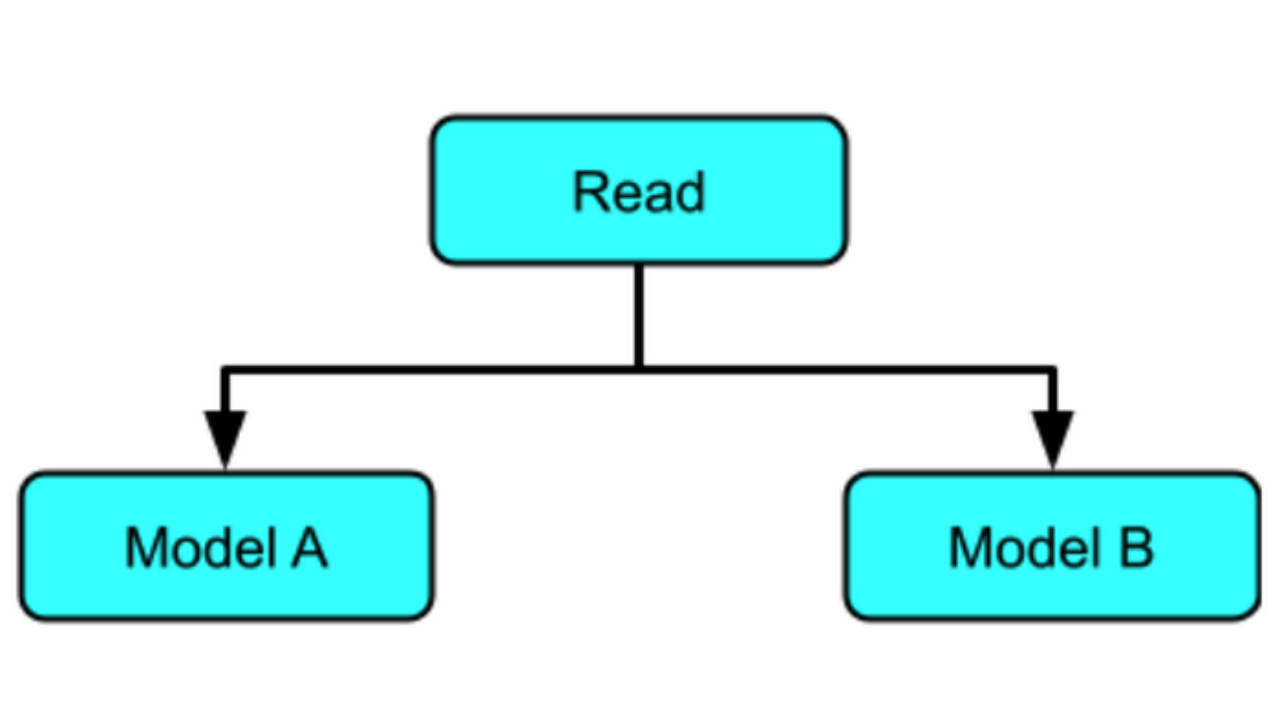
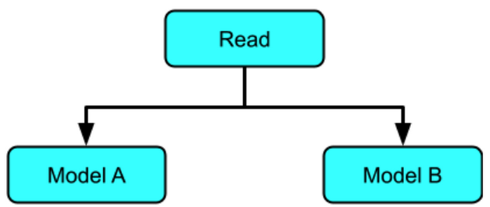
In part I of the series, the “join results from multiple models” pattern covered the various branching techniques in Apache Beam that make it possible to run data through multiple models.
Those techniques are applicable to RunInference API, which can easily be used by multiple branches within a pipeline, with the same or different models. This is similar in function to cascade ensembling, although here the data flows through multiple models in a single Apache Beam DAG.
Inference with multiple models in parallel
In this example, the same data is run through two different models: the one that we’ve been using to multiply by 5 and a new model, which will learn to multiply by 10.
"""
Create multiply by 10 table.

x is a range of values from 0 to 100.
y is a list of x * 10

value_to_predict includes a values outside of the training data
"""
x = numpy.arange( 0, 1000)
y = x * 10

# Create our labeled example file for 10 times table

example_ten_times_table = 'example_ten_times_table.tfrecord'

with tf.io.TFRecordWriter( example_ten_times_table ) as writer:
 for i in zip(x, y):
   example = ExampleProcessor().create_example_with_label(
       feature=i[0], label=i[1])
   writer.write(example.SerializeToString())

dataset = tf.data.TFRecordDataset(example_ten_times_table)
dataset = dataset.map(lambda e : tf.io.parse_example(e, RAW_DATA_TRAIN_SPEC))
dataset = dataset.map(lambda t : (t['x'], t['y']))
dataset = dataset.batch(100)
dataset = dataset.repeat()

model.fit(dataset, epochs=500, steps_per_epoch=10, verbose=0)

tf.keras.models.save_model(model,
                           save_model_dir_multiply_ten,
                           signatures=signature)
Now that we have two models, we apply them to our source data.
pipeline_options = PipelineOptions().from_dictionary(
                                     {'temp_location':f'gs://{bucket}/tmp'})

pipeline = beam.Pipeline(options=pipeline_options)

with pipeline as p:
 questions = p | beam.io.gcp.bigquery.ReadFromBigQuery(
                                   table=f'{project}:maths.maths_problems_1')

 multiply_five = ( questions
             | "CreateMultiplyFiveTuple" >>
             beam.Map(lambda x : (bytes('{}{}'.format(x['key'],' * 5'),'utf-8'),
                                   ExampleProcessor().create_example(x['value'])))

             | "Multiply Five" >> RunInference(
                 model_spec_pb2.InferenceSpecType(
                 saved_model_spec=model_spec_pb2.SavedModelSpec(
                                           model_path=save_model_dir_multiply)))
     )
 multiply_ten = ( questions
         | "CreateMultiplyTenTuple" >>
         beam.Map(lambda x : (bytes('{}{}'.format(x['key'],'* 10'), 'utf-8'),
                              ExampleProcessor().create_example(x['value'])))
         | "Multiply Ten" >> RunInference(
             model_spec_pb2.InferenceSpecType(
             saved_model_spec=model_spec_pb2.SavedModelSpec(
                                         model_path=save_model_dir_multiply_ten)))
 )
 _ = ((multiply_five, multiply_ten) | beam.Flatten()
                                    | beam.ParDo(PredictionWithKeyProcessor())
                                    | beam.Map(print))
Output:
key is b'first_question * 5' input is [105.] output is 524.0875854492188
key is b'second_question * 5' input is [108.] output is 539.0093383789062
key is b'third_question * 5' input is [1000.] output is 4975.75830078125
key is b'fourth_question * 5' input is [1013.] output is 5040.41943359375
key is b'first_question* 10' input is [105.] output is 1054.333984375
key is b'second_question* 10' input is [108.] output is 1084.3131103515625
key is b'third_question* 10' input is [1000.] output is 9998.0908203125
key is b'fourth_question* 10' input is [1013.] output is 10128.0009765625Inference with multiple models in sequence
In a sequential pattern, data is sent to one or more models in sequence, with the output from each model chaining to the next model.

Here are the steps:
- Read the data from BigQuery
- Map the data
- RunInference with multiply by 5 model
- Process the results
- RunInference with multiply by 10 model
- Process the results
pipeline_options = PipelineOptions().from_dictionary(
                                       {'temp_location':f'gs://{bucket}/tmp'})

pipeline = beam.Pipeline(options=pipeline_options)

def process_interim_inference(element : Tuple[
                                        bytes, prediction_log_pb2.PredictionLog
                                        ])-> Tuple[bytes, tf.train.Example]:

  key = '{} original input is {}'.format(
             element[0], str(tf.train.Example.FromString(
                 element[1].predict_log.request.inputs['examples'].string_val[0]
                 ).features.feature['x'].float_list.value[0]))

  value = ExampleProcessor().create_example(
              element[1].predict_log.response.outputs['output_0'].float_val[0])

  return (bytes(key,'utf-8'),value)

with pipeline as p:

 questions = p | beam.io.gcp.bigquery.ReadFromBigQuery(
                                   table=f'{project}:maths.maths_problems_1')

 multiply = ( questions
             | "CreateMultiplyTuple" >>
             beam.Map(lambda x : (bytes(x['key'],'utf-8'),
                                   ExampleProcessor().create_example(x['value'])))
             | "MultiplyFive" >> RunInference(
                 model_spec_pb2.InferenceSpecType(
                 saved_model_spec=model_spec_pb2.SavedModelSpec(
                                   model_path=save_model_dir_multiply)))

     )

 _ = ( multiply
         | "Extract result " >>
         beam.Map(lambda x : process_interim_inference(x))
         | "MultiplyTen" >> RunInference(
             model_spec_pb2.InferenceSpecType(
             saved_model_spec=model_spec_pb2.SavedModelSpec(
                             model_path=save_model_dir_multiply_ten)))
         | beam.ParDo(PredictionWithKeyProcessor())
         | beam.Map(print)
 )
Output:
key is b"b'first_question' original input is 105.0" input is [524.9771118164062] output is 5249.7822265625
key is b"b'second_question' original input is 108.0" input is [539.9765014648438] output is 5399.7763671875
key is b"b'third_question' original input is 1000.0" input is [4999.7841796875] output is 49997.9453125
key is b"b'forth_question' original input is 1013.0" input is [5064.78125] output is 50647.91796875Running the pipeline on Dataflow
Until now the pipeline has been run locally, using the direct runner, which is implicitly used when running a pipeline with the default configuration. The same examples can be run using the production Dataflow runner by passing in configuration parameters including --runner. Details and an example can be found here.
Here is an example of the multimodel pipeline graph running on the Dataflow service:
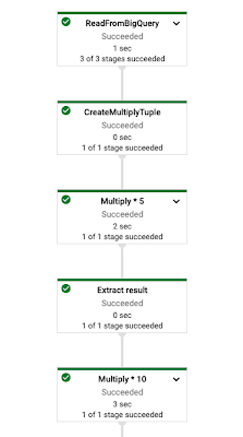
With the Dataflow runner you also get access to pipeline monitoring as well as metrics that have been output from the RunInference transform. The following table shows some of these metrics from a much larger list available from the library.

Conclusion
In this blog, part II of our series, we explored the use of the tfx-bsl RunInference within some common scenarios, from standard inference, to post processing and the use of RunInference API in multiple locations in the pipeline.
To learn more, review the Dataflow and TFX documentation, you can also try out TFX with Google Cloud AI platform pipelines..
Acknowledgements
None of this would be possible without the hard work of many folks across both the Dataflow TFX and TF teams. From the TFX and TF team we would especially like to thank Konstantinos Katsiapis, Zohar Yahav, Vilobh Meshram, Jiayi Zhao, Zhitao Li, and Robert Crowe. From the Dataflow team I would like to thank Ahmet Altay for his support and input throughout.
Michael Bronstein aims to unite the deep learning community
The ARA recipient is pioneering geometric deep learning, an approach that not only promises breakthroughs, but also a way to unify the machine learning “zoo”.Read More
Improving explainable AI’s explanations
Causal analysis improves both the classification accuracy and the relevance of the concepts identified by popular concept-based explanatory models.Read More
Sharpening Its Edge: U.S. Postal Service Opens AI Apps on Edge Network
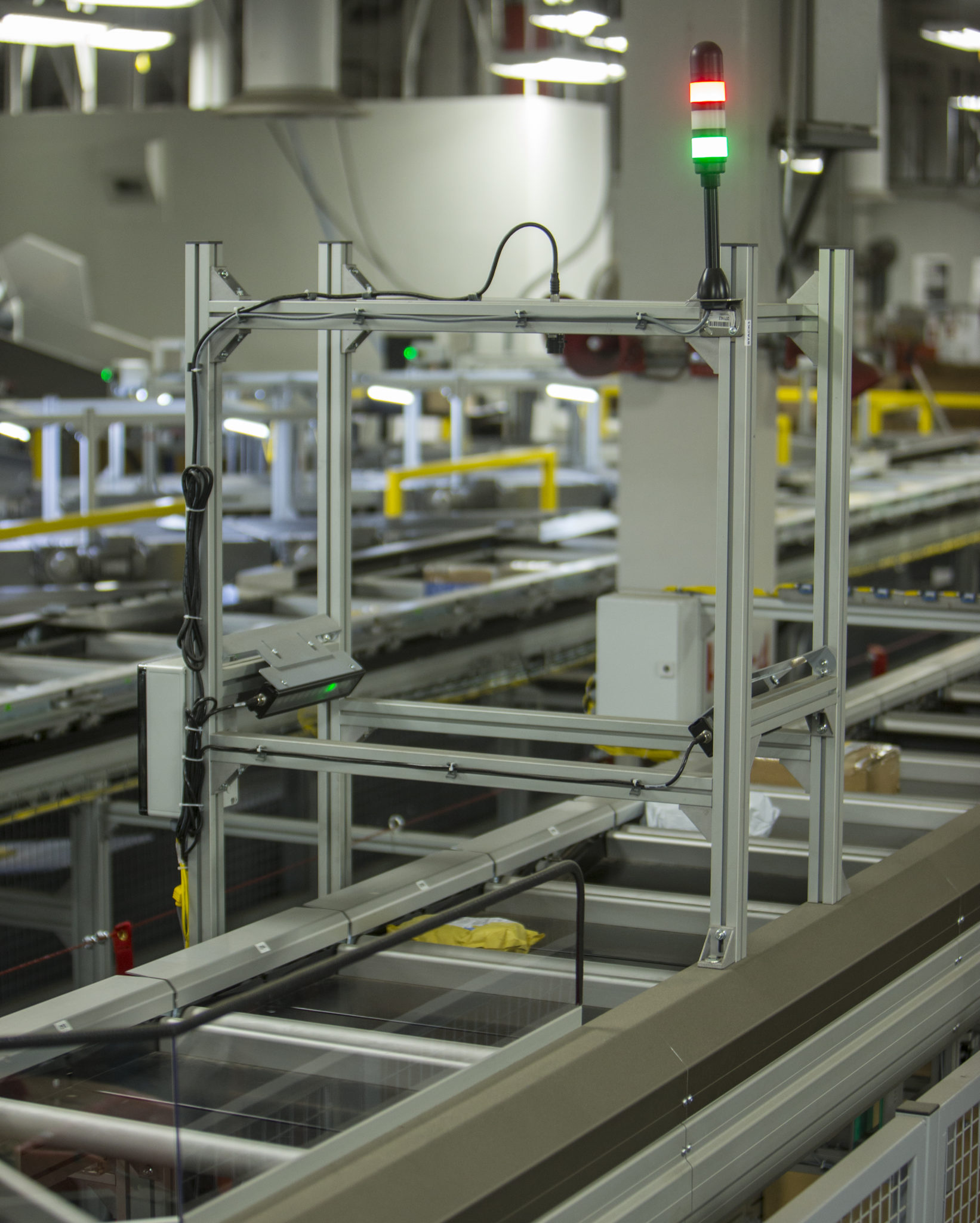
In 2019, the U.S. Postal Service had a need to identify and track items in its torrent of more than 100 million pieces of daily mail.
A USPS AI architect had an idea. Ryan Simpson wanted to expand an image analysis system a postal team was developing into something much broader that could tackle this needle-in-a-haystack problem.
With edge AI servers strategically located at its processing centers, he believed USPS could analyze the billions of images each center generated. The resulting insights, expressed in a few key data points, could be shared quickly over the network.
The data scientist, half a dozen architects at NVIDIA and others designed the deep-learning models needed in a three-week sprint that felt like one long hackathon. The work was the genesis of the Edge Computing Infrastructure Program (ECIP, pronounced EE-sip), a distributed edge AI system that’s up and running on the NVIDIA EGX platform at USPS today.
An AI Platform at the Edge
It turns out edge AI is a kind of stage for many great performances. ECIP is already running a second app that acts like automated eyes, tracking items for a variety of business needs.
“It used to take eight or 10 people several days to track down items, now it takes one or two people a couple hours,” said Todd Schimmel, the manager who oversees USPS systems including ECIP, which uses NVIDIA-Certified edge servers from Hewlett-Packard Enterprise.
Another analysis was even more telling. It said a computer vision task that would have required two weeks on a network of servers with 800 CPUs can now get done in 20 minutes on the four NVIDIA V100 Tensor Core GPUs in one of the HPE Apollo 6500 servers.
Today, each edge server processes 20 terabytes of images a day from more than 1,000 mail processing machines. Open source software from NVIDIA, the Triton Inference Server, acts as the digital mailperson, delivering the AI models each of the 195 systems need — when and how they need it.
Next App for the Edge
USPS put out a request for what could be the next app for ECIP, one that uses optical character recognition (OCR) to streamline its imaging workflow.
“In the past, we would have bought new hardware, software — a whole infrastructure for OCR; or if we used a public cloud service, we’d have to get images to the cloud, which takes a lot of bandwidth and has significant costs when you’re talking about approximately a billion images,” said Schimmel.
Today, the new OCR use case will live as a deep learning model in a container on ECIP managed by Kubernetes and served by Triton.
The same systems software smoothed the initial deployment of ECIP in the early weeks of the pandemic. Operators rolled out containers to get the first systems running as others were being delivered, updating them as the full network of nearly nodes was installed.
“The deployment was very streamlined,” Schimmel said. “We awarded the contract in September 2019, started deploying systems in February 2020 and finished most of the hardware by August — the USPS was very happy with that,” he added.
Triton Expedites Model Deliveries
Part of the software magic dust under ECIP’s hood, Triton automates the delivery of different AI models to different systems that may have different versions of GPUs and CPUs supporting different deep-learning frameworks. That saves a lot of time for edge AI systems like the ECIP network of almost 200 distributed servers.

The app that checks for mail items alone requires coordinating the work of more than a half dozen deep-learning models, each checking for specific features. And operators expect to enhance the app with more models enabling more features in the future.
“The models we have deployed so far help manage the mail and the Postal Service — it helps us maintain our mission,” Schimmel said.
A Pipeline of Edge AI Apps
So far, departments across USPS from enterprise analytics to finance and marketing have spawned ideas for as many as 30 applications for ECIP. Schimmel hopes to get a few of them up and running this year.
One would automatically check if a package carries the right postage for its size, weight and destination. Another one would automatically decipher a damaged barcode and could be online as soon as this summer.
“This has a benefit for us and our customers, letting us know where a specific parcel is at — it’s not a silver bullet, but it will fill a gap and boost our performance,” he said.
The work is part of a broader effort at USPS to explore its digital footprint and unlock the value of its data in ways that benefit customers.
“We’re at the very beginning of our journey with edge AI. Every day, people in our organization are thinking of new ways to apply machine learning to new facets of robotics, data processing and image handling,” he said.
Learn more about the benefits of edge computing and the NVIDIA EGX platform, as well as how NVIDIA’s edge AI solutions are transforming every industry.
Pictured at top: Postal Service employees perform spot checks to ensure packages are properly handled and sorted. Courtesy of U.S. Postal Service.
The post Sharpening Its Edge: U.S. Postal Service Opens AI Apps on Edge Network appeared first on The Official NVIDIA Blog.
GFN Thursday: 61 Games Join GeForce NOW Library in May
May’s shaping up to be a big month for bringing fan-favorites to GeForce NOW. And since it’s the first week of the month, this week’s GFN Thursday is all about the games members can look forward to joining the service this month.
In total, we’re adding 61 games to the GeForce NOW library in May, including 17 coming this week.
Joining This Week
This week’s additions include games from Remedy Entertainment, a classic Wild West FPS and a free title on Epic Games Store. Here are a few highlights:
Alan Wake (Steam)
A Dark Presence stalks the small town of Bright Falls, pushing Alan Wake to the brink of sanity in his fight to unravel the mystery and save his love.
Call of Juarez: Gunslinger (Steam)
From the dust of a gold mine to the dirt of a saloon, Call of Juarez Gunslinger is a real homage to Wild West tales. Live the epic and violent journey of a ruthless bounty hunter on the trail of the West’s most notorious outlaws.
Pine (Free on Epic Games Store until May 13)
An open-world action-adventure game set in a simulated world in which humans never reached the top of the food chain. Fight with or against a variety of species as you make your way to a new home for your human tribe.


Members can also look for the following titles later today:
- Alan Wake’s American Nightmare (Steam)
- Assetto Corsa (Steam)
- Beat Cop (Steam)
- Chronicon (Steam)
- Death Rally (Steam)
- Hitman 2: Silent Assassin (Steam)
- The Legend of Heroes: Trails of Cold Steel IV (Epic Games Store)
- MotoGP21 (Steam)
- Observer System Redux (Epic Games Store)
- Pacify (Steam)
- Project: Gorgon (Steam)
- THE SHORE (Steam)
- Steep (Steam)
- Tom Clancy’s Splinter Cell Blacklist (Steam)

More in May
This week is just the beginning. We have a giant list of titles joining GeForce NOW throughout the month, including:
- 41 Hours (Steam)
- Bad North (Steam, Epic Games Store)
- Battlefleet Gothic: Armada (Steam)
- Beyond Good & Evil (Steam)
- Breathedge (Steam, Epic Games Store)
- Bridge Constructor Portal (Steam)
- Chess Ultra (Steam)
- Child of Light (Ubisoft Connect)
- Cyber Hook (Steam)
- Deathsmiles (Steam)
- Enlisted (Native Launcher)
- Groove Coaster (Steam)
- Hearts of Iron 2 Complete (Steam)
- Hearts of Iron III (Steam)
- Hood: Outlaws & Legends (Steam, Epic Games Store)
- Hyperdrive Massacre (Steam)
- Imagine Earth (Steam)
- Just Die Already (Steam)
- Kill It With Fire (Steam)
- King’s Bounty: Dark Side (Steam)
- Last Epoch (Steam)
- Monopoly Plus (Ubisoft Connect)
- Monster Prom (Steam)
- Necromunda: Underhive Wars (Steam)
- OneShot (Steam)
- Ostriv (Steam)
- Outland (Steam)
- Outlast 2 (Steam)
- Red Wings: Ace of the Skies (Steam)
- Redout: Enhanced Edition (Steam)
- RIME (Steam)
- Sabotaj (Steam, only available in Europe)
- Space Crew (Steam)
- Space Invaders Extreme (Steam)
- Super Mecha Champions (Steam)
- Thea: The Awakening (Steam)
- Three Kingdoms: The Last Warlord (Steam)
- Tomb Raider Legend (Steam)
- Trainz Railroad Simulator 2019 (Steam)
- Valiant Hearts: The Great War (Ubisoft Connect)
- Warhammer 40,000: Inquisitor – Prophecy (Steam)
- Warhammer Age of Sigmar: Storm Ground (Steam)
- Warlock – Master of the Arcane (Steam)
- When Ski Lifts Go Wrong (Steam)
In Case You Missed It
In April, we added 27 more titles than shared on April 1. Check out these games, streaming straight from the cloud:
- Anno 2070 (Steam)
- Anno 2205 (Steam)
- AO Tennis 2 (Steam)
- Aron’s Adventure (Steam)
- Cardaclysm (Steam)
- Chinese Paladin: Sword and Fairy (Steam)
- Darksiders: Warmastered Edition (Epic Games Store)
- Darksiders II Deathinitive Edition (Epic Games Store)
- The Dungeon of Naheulbeuk: The Amulet of Chaos (Epic Games Store)
- Exanima (Steam)
- Far Cry 2: Fortune’s Edition (Epic Games Store)
- GoNNER (Epic Games Store)
- Nigate Tale (Steam)
- Port Royale 4 (Epic Games Store)
- Rayman Legends (Steam)
- Sheltered (Steam)
- Skyborn (Steam)
- SOMA (Epic Games Store)
- Stronghold Legends: Steam Edition (Steam)
- UNDER NIGHT IN-BIRTH Exe:Late[cl-r] (Steam)
- Vigil: The Longest Night (Steam)
- Warhammer 40,000: Inquisitor – Martyr (Steam)
- Werewolf: The Apocalypse – Heart of the Forest (Steam)
- Worms: Clan Wars (Steam)
- Yes, Your Grace (Steam, Epic Games Store)
- Yooka-Laylee and the Impossible Lair (Epic Games Store)
- Yuppie Psycho: Executive Edition (Steam)
Time to start planning your month, members. What are you going to play? Let us know on Twitter or in the comments below.
The post GFN Thursday: 61 Games Join GeForce NOW Library in May appeared first on The Official NVIDIA Blog.