Our research explored a new approach to an old problem: we reformulated principal component analysis (PCA), a type of eigenvalue problem, as a competitive multi-agent game we call EigenGame.Read More
Automatically scale Amazon Kendra query capacity units with Amazon EventBridge and AWS Lambda
Data is proliferating inside the enterprise and employees are using more applications than ever before to get their jobs done, in fact according to Okta Inc., the number of software apps deployed by large firms across all industries world-wide has increased 68%, reaching an average of 129 apps per company.
As employees continue to self-serve and the number of applications they use grows, so will the likelihood that critical business information will remain hard to find or get lost between systems, negatively impacting workforce productivity and operating costs.
Amazon Kendra is an intelligent search service powered by machine learning (ML). Unlike conventional search technologies, Amazon Kendra reimagines search by unifying unstructured data across multiple data sources as part of a single searchable index. It’s deep learning and natural language processing capabilities then make it easy for you to get relevant answers when you need them.
Amazon Kendra Enterprise Edition includes storage capacity for 500,000 documents (150 GB of storage) and a query capacity of 40,000 queries per day (0.5 queries per second), and allows you to adjust index capacity by increasing or decreasing your query and storage capacity units as needed.
However, usage patterns and business needs are not always predictable. In this post we’ll demonstrate how you can automatically scale your Amazon Kendra index based on a time schedule using Amazon EventBridge and AWS Lambda. By doing this you can increase capacity for peak usage, avoid service throttling, maintain flexibility, and control costs.
Solution overview
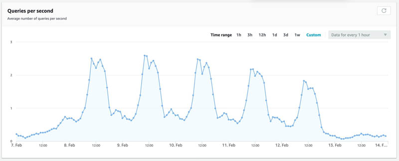
Amazon Kendra provides a dashboard that allows you to evaluate the average number of queries per second for your index. With this information, you can estimate the number of additional capacity units your workload requires at a specific point in time.
For example, the following graph shows that during business hours, a surge occurs in the average queries per second, but after hours, the number of queries reduces. We base our solution on this pattern to set up an EventBridge scheduled event that triggers the automatic scaling Lambda function.
The following diagram illustrates our architecture.

You can deploy the solution into your account two different ways:
- Deploy an AWS Serverless Application Model (AWS SAM) template:
- Clone the project from the aws-samples repository on GitHub and follow the instructions.
- Create the resources by using the AWS Management Console. In this post, we walk you through the following steps:
- Set up the Lambda function for scaling
- Configure permissions for the function
- Test the function
- Set up an EventBridge scheduled event
Set up the Lambda function
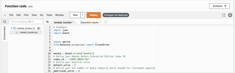
To create the Lambda function that we use for scaling, we create a function using the Python runtime (for this post, we use the Python 3.8 runtime).

Use the following code as the content of your lambda_function.py code:
#
# Copyright 2020 Amazon.com, Inc. or its affiliates. All Rights Reserved.
#
# Permission is hereby granted, free of charge, to any person obtaining a copy of this
# software and associated documentation files (the "Software"), to deal in the Software
# without restriction, including without limitation the rights to use, copy, modify,
# merge, publish, distribute, sublicense, and/or sell copies of the Software, and to
# permit persons to whom the Software is furnished to do so.
#
# THE SOFTWARE IS PROVIDED "AS IS", WITHOUT WARRANTY OF ANY KIND, EXPRESS OR IMPLIED,
# INCLUDING BUT NOT LIMITED TO THE WARRANTIES OF MERCHANTABILITY, FITNESS FOR A
# PARTICULAR PURPOSE AND NONINFRINGEMENT. IN NO EVENT SHALL THE AUTHORS OR COPYRIGHT
# HOLDERS BE LIABLE FOR ANY CLAIM, DAMAGES OR OTHER LIABILITY, WHETHER IN AN ACTION
# OF CONTRACT, TORT OR OTHERWISE, ARISING FROM, OUT OF OR IN CONNECTION WITH THE
# SOFTWARE OR THE USE OR OTHER DEALINGS IN THE SOFTWARE.
#

'''
 Changes the number of Amazon Kendra Enterprise Edition index capacity units

 Parameters
 ----------
 event : dict
 Lambda event

 Returns
 -------
 The additional capacity action or an error
'''

import json
import boto3
from botocore.exceptions import ClientError

# Variable declaration
KENDRA = boto3.client("kendra")
# Define your Amazon Kendra Enterprise Edition index ID
INDEX_ID = "<YOUR-INDEX-ID>"
# Define your baseline units
DEFAULT_UNITS = 0
# Define your the number of Query Capacity Units needed for increased capacity
ADDITIONAL_UNITS= 1


def add_capacity(INDEX_ID,capacity_units):
    try:
        response = KENDRA.update_index(
            Id=INDEX_ID,
            CapacityUnits={
                'QueryCapacityUnits': int(capacity_units),
                'StorageCapacityUnits': 0

            })
        return(response)
    except Exception as e:
        raise e


def reset_capacity(INDEX_ID,DEFAULT_UNITS):
    try:
        response = KENDRA.update_index(
            Id=INDEX_ID,
            CapacityUnits={
            'QueryCapacityUnits': DEFAULT_UNITS,
            'StorageCapacityUnits': 0
        })
    except Exception as e:
        raise e


def current_capacity(INDEX_ID):
    try:
        response = KENDRA.describe_index(
        Id=INDEX_ID)
        return(response)
    except Exception as e:
        raise e


def lambda_handler(event,context):
    print("Checking for query capacity units......")
    response = current_capacity(INDEX_ID)
    currentunits = response['CapacityUnits']['QueryCapacityUnits']
    print ("Current query capacity units are: "+str(currentunits))
    status = response['Status']
    print ("Current index status is: "+status)
    # If index is stuck in UPDATE state, don't attempt changing the capacity
    if status == "UPDATING":
        return ("Index is currently being updated. No changes have been applied")
    if status == "ACTIVE":
        if currentunits == 0:
            print ("Adding query capacity...")
            response = add_capacity(INDEX_ID,ADDITIONAL_UNITS)
            print(response)
            return response
        else:
            print ("Removing query capacity....")
            response = reset_capacity(INDEX_ID, DEFAULT_UNITS)
            print(response)
            return response
    else:
         response = "Index is not ready to modify capacity. No changes have been applied."
         return(response)
You must modify the following variables to match with your environment:
# Define your Amazon Kendra Enterprise Edition index ID
INDEX_ID = "<YOUR-INDEX-ID>"
# Define your baseline units
DEFAULT_UNITS = 1
# Define your the number of Query Capacity Units needed for increased capacity
ADDITIONAL_UNITS = 4
- INDEX_ID – The ID for your index; you can check it on the Amazon Kendra console.
- DEFAULT_UNITS – The number of query processing units that your Amazon Kendra Enterprise Edition requires to operate at minimum capacity. This number can range from 0–20 (you can request more capacity). 0 represents that no extra capacity units are provisioned to your Amazon Kendra Enterprise Edition index, which leaves it with a default capacity of 0.5 queries per second.
- ADDITIONAL_UNITS – The number of query capacity units you require at those times where additional capacity is required. This value can range from 1–20 (you can request additional capacity).
Configure function permissions
To query the status of your index and to modify the number of query capacity units, you need to attach a policy to your Lambda function AWS Identity and Access Management (IAM) execution role with those permissions.
- On the Lambda console, navigate to your function.
- On the Permissions tab, choose the execution role.

The IAM console opens automatically.
- On the Permissions tab, choose Attach policies.

- Choose Create policy.
A new tab opens.
- On the JSON tab, add the following content (make sure to provide your account and user information):
{
    "Version": "2012-10-17",
    "Statement": [
        {
            "Sid": "MyPolicy",
            "Effect": "Allow",
            "Action": [
                "kendra:UpdateIndex",
                "kendra:DescribeIndex"
            ],
            "Resource": "arn:aws:kendra:<YOUR-AWS-REGION>:<YOUR-ACCOUNT-ID>:index/<YOUR-INDEX-ID>"
        }
    ]
}
- Choose Next: Tags.
- Choose Next: Review.
- For Name, enter a policy name (for this post, we use
AmazonKendra_UpdateIndex). - Choose Create policy.
- On the Attach permissions page, choose the refresh icon.
- Filter to find the policy you created.
- Select the policy and choose Attach policy.

Test the function
You can test your Lambda function by running a test event. For more information, see Invoke the Lambda function.
- On the Lambda console, navigate to your function.
- Create a new test event by choosing Test.

- Select Create new test event.
- For Event template, because your function doesn’t require any input from the event, you can choose the
hello-worldevent template.
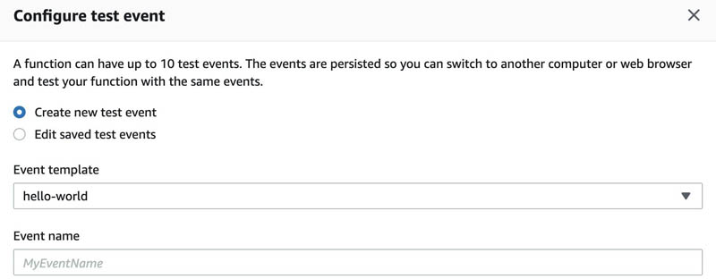
- Choose Create.
- Choose Test.
On the Lambda function logs, you can see the following messages:
Function Logs
START RequestId: 9b2382b7-0229-4b2b-883e-ba0f6b149513 Version: $LATEST
Checking for capacity units......
Current capacity units are: 1
Current index status is: ACTIVE
Adding capacity...
Set up an EventBridge scheduled event
An EventBridge scheduled event is an EventBridge event that is triggered on a regular schedule. This section shows how to create an EventBridge scheduled event that runs every day at 7 AM UTC and at 8 PM UTC to trigger the kendra-index-scaler Lambda function. This allows your index to scale up with the additional query capacity units at 7 AM and scale down at 8 PM.
When you set up EventBridge scheduled events, you do so for the UTC time zone, so you need to calculate the time offset. For example, to run the event at 7 AM Central Standard Time (CST), you need to set the time to 1 PM UTC. If you want to accommodate for daylight savings, you have to create a different rule to account for the difference.
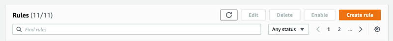
- On the EventBridge console, in the navigation pane, under Events, choose Rules.
- Choose Create rule.
- For Name, enter a name for your rule (for this post, we use
kendra-index-scaler).

- In the Define pattern section, select Schedule.
- Select Cron expression and enter
0 7,20 * * ? *.
We use this cron expression to trigger the EventBridge event every day at 7 AM and 8 PM.
- In the Select event bus section, select AWS default event bus.

- In the Select targets section, for Target, choose Lambda function.
- For Function, enter the function you created earlier (
lambda_function_kendra_index_handler).

- Choose Create.
You can check Amazon CloudWatch Logs for the lambda_function_kendra_index_handler function and see how it behaves depending on your index’s query capacity units.

Conclusion
In this post, you deployed a mechanism to automatically scale additional query processing units for your Amazon Kendra Enterprise Edition index.
As a next step, you could periodically review your usage patterns in order to plan the schedule to accommodate your query volume. To learn more about Amazon Kendra’s use cases, benefits, and how to get started with it, visit the webpage!
About the Authors
 Juan Bustos is an AI Services Specialist Solutions Architect at Amazon Web Services, based in Dallas, TX. Outside of work, he loves spending time writing and playing music as well as trying random restaurants with his family.

Tapodipta Ghosh is a Senior Architect. He leads the Content And Knowledge Engineering Machine Learning team that focuses on building models related to AWS Technical Content. He also helps our customers with AI/ML strategy and implementation using our AI Language services like Amazon Kendra.
 Tom McMahon is a Product Marketing Manager on the AI Services team at AWS. He’s passionate about technology and storytelling and has spent time across a wide-range of industries including healthcare, retail, logistics, and ecommerce. In his spare time he enjoys spending time with family, music, playing golf, and exploring the amazing Pacific northwest and its surrounds.
Automate multi-modality, parallel data labeling workflows with Amazon SageMaker Ground Truth and AWS Step Functions
This is the first in a two-part series on the Amazon SageMaker Ground Truth hierarchical labeling workflow and dashboards. In Part 1, we look at creating multi-step labeling workflows for hierarchical label taxonomies using AWS Step Functions. In Part 2 (coming soon), we look at how to build dashboards for analyzing dataset annotations and worker performance metrics on data lakes generated as output from the complex workflows and derive insights.
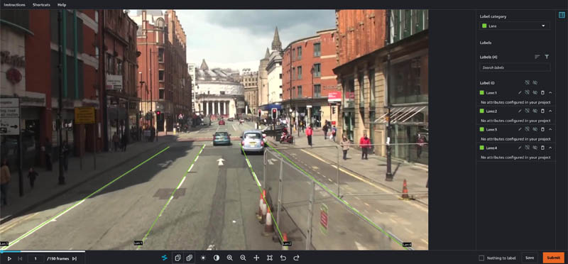
Data labeling often requires a single data object to include multiple types of annotations, or multi-type, such as 2D boxes (bounding boxes), lines, and segmentation masks, all on a single image. Additionally, to create high-quality machine learning (ML) models using labeled data, you need a way to monitor the quality of the labels. You can do this by creating a workflow in which labeled data is audited and adjusted as needed. This post introduces a solution to address both of these labeling challenges using an automotive dataset, and you can extend this solution for use with any type of dataset.
For our use case, assume you have a large quantity of automotive video data filmed from one or more angles on a moving vehicle (for example, some Multi-Object Tracking (MOT) scenes) and you want to annotate the data using multiple types of annotations. You plan to use this data to train a cruise control, lane-keeping ML algorithm. Given the task at hand, it’s imperative that you use high-quality labels to train the model.
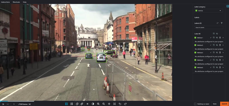
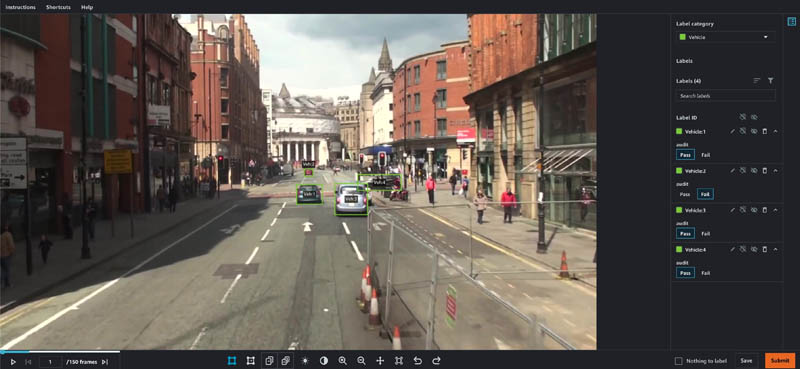
First, you must identify the types of annotations you want to add to your video frames. Some of the most important objects to label for this use case are other vehicles in the frame, road boundaries, and lanes. To do this, you define a hierarchical label taxonomy, which defines the type of labels you want to add to each video, and the order in which you want the labels to be added. The Ground Truth video tracking labeling job supports bounding box, polyline, polygon, and keypoint annotations. In this use case, vehicles are annotated using 2-dimensional boxes, or bounding boxes, and road boundaries and curves are annotated with a series of flexible lines segments, referred to as polylines.
Second, you need to establish a workflow to ensure label quality. To do this, you can create an audit workflow to verify the labels generated by your pipeline are of high enough quality to be useful for model training. In this audit workflow, you can greatly improve label accuracy by building a multi-step review pipeline that allows annotations to be audited, and if necessary, adjusted by a second reviewer who may be a subject matter expert.
Based on the size of the dataset and data objects, you should also consider the time and resources required to create and maintain this pipeline. Ideally, you want this series of labeling jobs to be started automatically, only requiring human operation to specify the input data and workflow.
The solution used in this post uses Ground Truth, AWS CloudFormation, Step Functions, and Amazon DynamoDB to create a series of labeling jobs that run in a parallel and hierarchical fashion. You use a hierarchical label taxonomy to create labeling jobs of different modalities (polylines and bounding boxes), and you add secondary human review steps to improve annotation quality and final results.
For this post, we demonstrate the solution in the context of the automotive space, but you can easily apply this general pipeline to labeling pipelines involving images, videos, text, and more. In addition, we demonstrate a workflow that is extensible, allowing you to reduce the total number of frames that need human review by adding automated quality checks and maintaining data quality at scale. In this use case, we use these checks to find anomalies in MOT time series data like video object tracking annotations.
We walk through a use case in which we generate multiple types of annotations for an automotive scene. Specifically, we run four labeling jobs per input video clip: an initial labeling of vehicles, initial labeling of lanes, and then an adjustment job per initial job with a separate quality assurance workforce.
We demonstrate the various extension points in our Step Function workflow that can allow you to run automated quality assurance checks. This allows for clip filtering between and after jobs have completed, which can result in high-quality annotations for a fraction of the cost.
AWS services used to implement this solution
This solution creates and manages Ground Truth labeling jobs to label video frames using multiple types of annotations. Ground Truth has native support for video datasets through its video frame object tracking task type.
This task type allows workers to create annotations across a series of video frames, providing tools to predict the next location of a bounding box in subsequent frames. It also supports multiple annotation types such as bounding boxes or polylines through the label category configuration files provided during job creation. We use these tools in this tutorial, running a job for vehicle bounding boxes and a job for lane polylines.
We use Step Functions to manage the labeling job. This solution abstracts labeling job creation so that you specify the overall workflow you want to run using a hierarchical label taxonomy, and all job management is handled by Step Functions.
The solution is implemented using CloudFormation templates that you can deploy in your AWS account. The interface to the solution is an API managed by Amazon API Gateway, which provides the ability to submit annotation tasks to the solution, which are then translated into Ground Truth labeling jobs.
Estimated costs
By deploying and using this solution, you incur the maximum cost of approximately $20 other than human labeling costs because it only uses fully managed compute resources on demand. Amazon Simple Storage Service (Amazon S3), AWS Lambda, Amazon SageMaker, API Gateway, Amazon Simple Notification Service (Amazon SNS), Amazon Simple Queue Service (Amazon SQS), AWS Glue, and Step Functions are included in the AWS Free Tier, with charges for additional use. For more information, see the following pricing pages:
Ground Truth pricing depends on the type of workforce that you use. If you’re a new user of Ground Truth, we suggest that you use a private workforce and include yourself as a worker to test your labeling job configuration. For more information, see Amazon SageMaker Ground Truth pricing.
Solution overview
In this two-part series, we discuss an architecture pattern that allows you to build a pipeline for orchestrating multi-step data labeling workflows that have workers add different types of annotation in parallel using Ground Truth. You also learn how you can analyze the dataset annotations produced by the workflow as well as worker performance. The first post covers the Step Functions workflow that automates advanced ML data labeling workflows using Ground Truth for chaining and hierarchical label taxonomies. The second post describes how to build data lakes on dataset annotations from Ground Truth and worker metrics and use these data lakes to derive insights or analyze the performance of your workers and dataset annotation quality using advanced analytics.
The following diagram depicts the hierarchical workflow, which you can use to run groups of labeling jobs in sequential steps, or levels, in which each labeling job in a single level runs in parallel.

The solution is composed of two main parts:
- Use an API to trigger the orchestration workflow.
- Run the individual steps of the workflow to achieve the labeling pipeline.
Trigger the orchestration workflow with an API
The CloudFormation template launched in this solution uses API Gateway to expose an endpoint for you to trigger batch labeling jobs. After you send the post request to the API Gateway endpoint, it runs a Lambda function to trigger the workflow.
The following table contains the two main user-facing APIs relevant to running batch, which represents multi-level labeling jobs.
| URL | Request Type | Description |
| {endpointUrl}/batch/create | POST | API triggers a new batch of labeling jobs |
| {endpointUrl}/batch/show | GET | APIs describe current state of the batch job run |
Run the workflow
For the orchestration of steps, we use Step Functions as a managed solution. When the batch job creation API is triggered, a Lambda function triggers a Step Functions workflow like the following. This begins the annotation input processing.
Let’s discuss the steps in more detail.
Transformation step
The first step is to preprocess the data. The current implementation converts the notebook inputs into the internal manifest file data type shared across multiple steps. This step doesn’t currently perform any complex processing, but you can further customize this step by adding custom data preprocessing logic to this function. For example, if your dataset was encoded in raw videos, you could perform frame splitting and manifest generation within transformation rather than in a separate notebook. Alternatively, if you’re using this solution to create a 3D point cloud labeling pipeline, you may want to add logic to extract pose data in a world coordinate system using the camera and LiDAR extrinsic matrices.
TriggerLabelingFirstLevel
When the data preprocessing is complete, the Ground Truth API operation CreateLabelingJob is used to launch labeling jobs. These labeling jobs are responsible for annotating datasets that are tied to the first level.
CheckForFirstLevelComplete
This step waits for the FIRST_LEVEL Ground Truth labeling jobs triggered from the TriggerLabelingFirstStep. When the job trigger is complete, this step waits for all the created labeling jobs to complete. An external listener Lambda function monitors the status of the labeling jobs, and when all the pending labeling jobs are done, it runs the sendTokenSucess API to signal to this state to proceed to the next step. Failure cases are handled using appropriate error clauses and timeouts in the step definition.
SendSecondLevelSNSAndCheckResponse
This step performs postprocessing on the output of the first-level job. For example, if your requirements are to only send 10% of frames to the adjustment jobs, you can implement this logic here by filtering the set of outputs from the first job.
TriggerLabelingSecondLevel
When the data postprocessing from the first-level is complete, CreateLabelingJobs is used to launch labeling jobs to complete annotations at the second level. At this stage, a private workforce reviews the quality of annotations of the first-level labeling jobs and updates annotations as needed.
CheckForSecondLevelComplete
This step is the same wait step as CheckForFirstLevelComplete, but this step simply waits for the jobs that are created from the second level.
SendThirdLevelSNSAndCheckResponse
This step is the same post-processing step as SendSecondLevelSNSAndCheckResponse, but this step does the postprocessing of the second-level output and feeds as input to the third-level labeling job.
TriggerLabelingThirdLevel
This is the same logic as TriggerLabelingSecondLevel, but the labeling jobs are triggered that are annotated as third level. At this stage, the private workforce is updating annotations for quality of the second-level labeling job.
CopyLogsAndSendBatchCompleted
This Lambda function logs and sends SNS messages to notify users that the batch is complete. It’s also a placeholder for any post-processing logic that you may want to run. Common postprocessing includes transforming the labeled data into a format compatible with a customer-specific data format.
Prerequisites
Before getting started, make sure you have the following prerequisites:
- An AWS account.
- A notebook AWS Identity and Access Management (IAM) role with the permissions required to complete this walkthrough. Your IAM role must have the required permissions attached. If you don’t require granular permission, attach the following AWS managed policies:
AmazonS3FullAccessAmazonAPIGatewayInvokeFullAccessAmazonSageMakerFullAccess
- Familiarity with Ground Truth, AWS CloudFormation, and Step Functions.
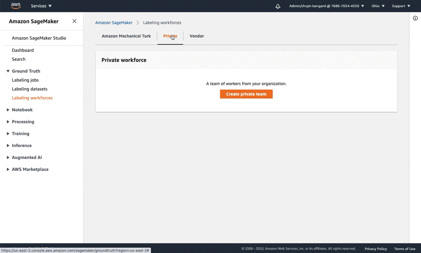
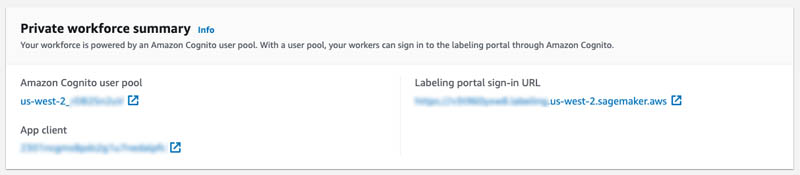
- A SageMaker workforce. For this post, we use a private workforce. You can create a workforce on the SageMaker console. Note the Amazon Cognito user pool identifier and the app client identifier after your workforce is created. You use these values to tell the CloudFormation stack deployment which workforce to create work teams, which represent the group of labelers. You can find these values in the Private workforce summary section on the console after you create your workforce, or when you call DescribeWorkteam.
The following GIF demonstrates how to create a private workforce. For step-by-step instructions, see Create an Amazon Cognito Workforce Using the Labeling Workforces Page.
Launch the CloudFormation stack
Now that we’ve seen the structure of the solution, we deploy it into our account so we can run an example workflow. All our deployment steps are managed by AWS CloudFormation—it creates resources in Lambda, Step Functions, DynamoDB, and API Gateway for you.
You can launch the stack in AWS Region us-east-1 on the CloudFormation console by choosing Launch Stack:
![]()
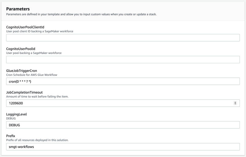
On the CloudFormation console, select Next, and then modify the following template parameters to customize the solution.
You can locate the CognitoUserPoolClientId and CognitoUserPoolId in the SageMaker console.
- CognitoUserPoolClientId: App client ID of your private workforce.
- CognitoUserPoolId: ID of the user pool associated with your private workforce.
To locate these values in the console:
- Open the SageMaker console at https://console.aws.amazon.com/sagemaker/
- Select Labeling workforces in the navigation pane.
- Choosing the Private
- Use the values in the Private work team summary Use the App client for the CognitoUserPoolClientId and use Amazon Cognito user pool for the CognitoUserPoolId.
For this tutorial, you can use the default values for the following parameters.
- GlueJobTriggerCron: Cron expression to use when scheduling reporting AWS Glue cron job. The results from annotations generated with SageMaker Ground Truth and worker performance metrics are used to create a dashboard in Amazon QuickSight. This will be explained in detail as part of second part. The outputs from SageMaker annotations and worker performance metrics shows up in Athena queries after processing the data with AWS Glue. By default, AWS Glue cron jobs run every hour.
- JobCompletionTimeout: Number of seconds to wait before treating a labeling job as failed and moving to the BatchError state.
- LoggingLevel: This is used internally and can be ignored. Logging level to change verbosity of logs. Accepts values DEBUG and PROD.
Prefix: A prefix to use when naming resources used to creating and manage labeling jobs and worker metrics.
To launch the stack in a different AWS Region, use the instructions found in the README of the GitHub repository.
After you deploy the solution, two new work teams are in the private workforce you created earlier: smgt-workflow-first-level and smgt-workflow-second-level. These are the default work teams used by the solution if no overrides are specified, and the smgt-workflow-second-level work team is used for labeling second-level and third-level jobs. You should add yourself to both work teams to see labeling tasks created by the solution. To learn how to add yourself to a private work team, see Add or Remove Workers.
You also need to go the the API Gateway console and look for the deployed API prefixed with smgt-workflow and note its ID. The notebook needs to reference this ID so it can determine which API URL to call.
Launch the notebook
After you deploy the solution into your account, you’re ready to launch a notebook to interact with it and start new workflows. In this section, we walk through the following steps:
- Set up and access the notebook instance.
- Obtain the example dataset.
- Prepare Ground Truth input files.
Set up the SageMaker notebook instance
In this example notebook, you learn how to map a simple taxonomy consisting of a vehicle class and a lane class to Ground Truth label category configuration files. A label category configuration file is used to define the labels that workers use to annotation your images. Next, you learn how to launch and configure the solution that runs the pipeline using a CloudFormation template. You can also further customize this code, for example by customizing the batch creation API call to run labeling for a different combination of task types.
To create a notebook instance and access the notebook used in this post, complete the following steps:
- Create a notebook instance with the following parameters:
- Use ml.t2.medium to launch the notebook instance.
- Increase the ML storage volume size to at least 10 GB.
- Select the notebook IAM role described in prerequisites. This role allows your notebook to upload your dataset to Amazon S3 and call the solution APIs.
- Open Jupyter Lab or Jupyter to access your notebook instances.
- In Jupyter, choose the SageMaker Examples In Jupyter Lab, choose the SageMaker icon.
- Choose Ground Truth Labeling Jobs and then choose the job sagemaker_ground_truth_workflows.ipynb.
- If you’re using Jupyter, choose Use to copy the notebook to your instance and run it. If you’re in Jupyter lab, choose Create a Copy.
Obtain the example dataset
Complete the following steps to set up your dataset:
- Download MOT17.zip using the Download Dataset section of the notebook.
This download is approximately 5 GB and takes several minutes.
- Unzip MOT17.zip using the notebook’s Unzip dataset
- Under the Copy Data to S3 header, run the cell to copy one set of video frames dataset to Amazon S3.
Prepare the Ground Truth input files
To use the solution, we need to create a manifest file. This file tells Ground Truth where your dataset is. We also need two label category configuration files to describe our label names, and the labeling tool to use for each (bounding box or polyline).
- Run the cells under Generate Manifest to obtain a list of frames in a video from the dataset. We take 150 frames at half the frame rate of the video as an example.
- Continue running cells under Generate Manifest to build a sequence file describing our video frames, and then to create a manifest file referring to our sequence file.
- Run the cell under Generate Label Category Configuration Files to create two new files: a vehicle label configuration file (which uses the bounding box tool), and a lane label configuration file (which uses the polyline tool).
- Copy the manifest file and label the category configuration files to Amazon S3 by running the Send data to S3
At this point, you have prepared all inputs to the labeling jobs and are ready to begin operating the solution.
To learn more about Ground Truth video frame labeling jobs and chaining, see the following references:
Run an example workflow
In this section, we walk through the steps to run an example workflow on the automotive dataset. We create a multi-modality workflow, perform both initial and audit labeling, then view our completed annotations.
Create a workflow batch
This solution orchestrates a workflow of Ground Truth labeling jobs to run both video object tracking bounding box jobs and polyline jobs, as well as automatically create adjustment jobs after the initial labeling. This workflow batch is configured through the batch_create API available to the solution.
Run the cell under Batch Creation Demo in the notebook. This passes your input manifest and label category configuration S3 URIs to a new workflow batch.
The cell should output the ID of the newly created workflow batch, for example:
Batch processor successfully triggered with BatchId : nb-ccb0514cComplete the first round of labeling tasks
To simulate workers completing labeling, we log in as a worker in the first-level Ground Truth work team and complete the labeling task.
- Run the cell under Sign-in To Worker Portal to get a link to log in to the worker portal.
An invitation should have already been sent to your email address if you invited yourself to the solution-generated first-level and second-level work teams.
- Log in and wait for the tasks to appear in the worker portal.
Two tasks should be available, one with ending in vehicle and one ending in lane, corresponding to the two jobs we created during workflow batch creation.
- Open each task and add some dummy labels by choosing and dragging on the image frames.
- Choose Submit on each task.
Complete the second round of labeling tasks
Our workflow specified we wanted adjustment jobs auto-launched for each first-level job. We now complete the second round of labeling tasks.
- Still in the worker portal, wait for tasks with
vehicle-auditandlane-auditto appear. - Open each task in the worker portal, noting that the prior level’s labels are still visible.
These adjustment tasks could be performed by a more highly trained quality assurance group in a different work team.
- Make adjustments as desired and choose Pass or Fail on each annotation.
- When you’re finished, choose Submit.

View the completed annotations
We can view details about the completed workflow batch by running the batch show API.
- Run the cell under Batch Show Demo.
This queries the solution’s database for all complete workflow run batches, and should output your batch ID when your batch is complete.
- We can get more specific details about a batch by running the cell under Batch Detailed Show Demo.
This takes the ID of a batch in the system and returns status information and the locations of all input and output manifests for each created job.
- Copy and enter the field
jobOutputS3Urlfor any of the jobs and verify the manifest file for that job is downloaded.
This file contains a reference to your input data sequence as well as the S3 URI of the output annotations for each sequence.
Final results
When all labeling jobs in the pipeline are complete, an SNS message is published on the default status SNS topic. You can subscribe to SNS topics using an email address for verifying the solution’s functionality. The message includes the batch ID used during batch creation, a message about the batch completion, and the same information the batch/show API provides under a batchInfo key. You can parse this message to extract metadata about the completed labeling jobs in the second level of the pipeline.
{
    "batchId": "nb-track-823f6d3e",
    "message": "Batch processing has completed successfully.",
    "batchInfo": {
        "batchId": "nb-track-823f6d3e",
        "status": "COMPLETE",
        "inputLabelingJobs": [
            {
                "jobName": "nb-track-823f6d3e-vehicle",
                "taskAvailabilityLifetimeInSeconds": "864000",
                "inputConfig": {
                    "inputManifestS3Uri": "s3://smgt-workflow-1-322552456788-us-west-2-batch-input/tracking_manifests/MOT17-13-SDP.manifest"
                },
                "jobModality": "VideoObjectTracking",
                "taskTimeLimitInSeconds": "604800",
                "maxConcurrentTaskCount": "100",
                "workteamArn": "arn:aws:sagemaker:us-west-2:322552456788:workteam/private-crowd/smgt-workflow-1-first-level",
                "jobType": "BATCH",
                "jobLevel": "1",
                "labelCategoryConfigS3Uri": "s3://smgt-workflow-1-322552456788-us-west-2-batch-input/tracking_manifests/vehicle_label_category.json"
            },
            {
                "jobName": "nb-track-823f6d3e-lane",
                "taskAvailabilityLifetimeInSeconds": "864000",
                "inputConfig": {
                    "inputManifestS3Uri": "s3://smgt-workflow-1-322552456788-us-west-2-batch-input/tracking_manifests/MOT17-13-SDP.manifest"
                },
                "jobModality": "VideoObjectTracking",
                "taskTimeLimitInSeconds": "604800",
                "maxConcurrentTaskCount": "100",
                "workteamArn": "arn:aws:sagemaker:us-west-2:322552456788:workteam/private-crowd/smgt-workflow-1-first-level",
                "jobType": "BATCH",
                "jobLevel": "1",
                "labelCategoryConfigS3Uri": "s3://smgt-workflow-1-322552456788-us-west-2-batch-input/tracking_manifests/lane_label_category.json"
            },
            {
                "jobName": "nb-track-823f6d3e-vehicle-audit",
                "taskAvailabilityLifetimeInSeconds": "864000",
                "inputConfig": {
                    "chainFromJobName": "nb-track-823f6d3e-vehicle"
                },
                "jobModality": "VideoObjectTrackingAudit",
                "taskTimeLimitInSeconds": "604800",
                "maxConcurrentTaskCount": "100",
                "workteamArn": "arn:aws:sagemaker:us-west-2:322552456788:workteam/private-crowd/smgt-workflow-1-first-level",
                "jobType": "BATCH",
                "jobLevel": "2"
            },
            {
                "jobName": "nb-track-823f6d3e-lane-audit",
                "taskAvailabilityLifetimeInSeconds": "864000",
                "inputConfig": {
                    "chainFromJobName": "nb-track-823f6d3e-lane"
                },
                "jobModality": "VideoObjectTrackingAudit",
                "taskTimeLimitInSeconds": "604800",
                "maxConcurrentTaskCount": "100",
                "workteamArn": "arn:aws:sagemaker:us-west-2:322552456788:workteam/private-crowd/smgt-workflow-1-first-level",
                "jobType": "BATCH",
                "jobLevel": "2"
            }
        ],
        "firstLevel": {
            "status": "COMPLETE",
            "numChildBatches": "2",
            "numChildBatchesComplete": "2",
            "jobLevels": [
                {
                    "batchId": "nb-track-823f6d3e-first_level-nb-track-823f6d3e-lane",
                    "batchStatus": "COMPLETE",
                    "labelingJobName": "nb-track-823f6d3e-lane",
                    "labelAttributeName": "nb-track-823f6d3e-lane-ref",
                    "labelCategoryS3Uri": "s3://smgt-workflow-1-322552456788-us-west-2-batch-input/tracking_manifests/lane_label_category.json",
                    "jobInputS3Uri": "s3://smgt-workflow-1-322552456788-us-west-2-batch-input/tracking_manifests/MOT17-13-SDP.manifest",
                    "jobInputS3Url": "https://smgt-workflow-1-322552456788-us-west-2-batch-input.s3.amazonaws.com/tracking_manifests/MOT17-13-SDP.manifest?...",
                    "jobOutputS3Uri": "s3://smgt-workflow-1-322552456788-us-west-2-batch-processing/batch_manifests/VideoObjectDetection/nb-track-823f6d3e-first_level-nb-track-823f6d3e-lane/output/nb-track-823f6d3e-lane/manifests/output/output.manifest",
                    "jobOutputS3Url": "https://smgt-workflow-1-322552456788-us-west-2-batch-processing.s3.amazonaws.com/batch_manifests/VideoObjectDetection/nb-track-823f6d3e-first_level-nb-track-823f6d3e-lane/output/nb-track-823f6d3e-lane/manifests/output/output.manifest?..."
                },
                {
                    "batchId": "nb-track-823f6d3e-first_level-nb-track-823f6d3e-vehicle",
                    "batchStatus": "COMPLETE",
                    "labelingJobName": "nb-track-823f6d3e-vehicle",
                    "labelAttributeName": "nb-track-823f6d3e-vehicle-ref",
                    "labelCategoryS3Uri": "s3://smgt-workflow-1-322552456788-us-west-2-batch-input/tracking_manifests/vehicle_label_category.json",
                    "jobInputS3Uri": "s3://smgt-workflow-1-322552456788-us-west-2-batch-input/tracking_manifests/MOT17-13-SDP.manifest",
                    "jobInputS3Url": "https://smgt-workflow-1-322552456788-us-west-2-batch-input.s3.amazonaws.com/tracking_manifests/MOT17-13-SDP.manifest?...",
                    "jobOutputS3Uri": "s3://smgt-workflow-1-322552456788-us-west-2-batch-processing/batch_manifests/VideoObjectTracking/nb-track-823f6d3e-first_level-nb-track-823f6d3e-vehicle/output/nb-track-823f6d3e-vehicle/manifests/output/output.manifest",
                    "jobOutputS3Url": "https://smgt-workflow-1-322552456788-us-west-2-batch-processing.s3.amazonaws.com/batch_manifests/VideoObjectTracking/nb-track-823f6d3e-first_level-nb-track-823f6d3e-vehicle/output/nb-track-823f6d3e-vehicle/manifests/output/output.manifest?..."
                }
            ]
        },
        "secondLevel": {
            "status": "COMPLETE",
            "numChildBatches": "2",
            "numChildBatchesComplete": "2",
            "jobLevels": [
                {
                    "batchId": "nb-track-823f6d3e-second_level-nb-track-823f6d3e-vehicle-audit",
                    "batchStatus": "COMPLETE",
                    "labelingJobName": "nb-track-823f6d3e-vehicle-audit",
                    "labelAttributeName": "nb-track-823f6d3e-vehicle-audit-ref",
                    "labelCategoryS3Uri": "s3://smgt-workflow-1-322552456788-us-west-2-batch-processing/label_category_input/nb-track-823f6d3e-second_level-nb-track-823f6d3e-vehicle-audit/category-file.json",
                    "jobInputS3Uri": "s3://smgt-workflow-1-322552456788-us-west-2-batch-processing/batch_manifests/VideoObjectTracking/nb-track-823f6d3e-first_level-nb-track-823f6d3e-vehicle/output/nb-track-823f6d3e-vehicle/manifests/output/output.manifest",
                    "jobInputS3Url": "https://smgt-workflow-1-322552456788-us-west-2-batch-processing.s3.amazonaws.com/batch_manifests/VideoObjectTracking/nb-track-823f6d3e-first_level-nb-track-823f6d3e-vehicle/output/nb-track-823f6d3e-vehicle/manifests/output/output.manifest?...",
                    "jobOutputS3Uri": "s3://smgt-workflow-1-322552456788-us-west-2-batch-processing/batch_manifests/VideoObjectTrackingAudit/nb-track-823f6d3e-second_level-nb-track-823f6d3e-vehicle-audit/output/nb-track-823f6d3e-vehicle-audit/manifests/output/output.manifest",
                    "jobOutputS3Url": "https://smgt-workflow-1-322552456788-us-west-2-batch-processing.s3.amazonaws.com/batch_manifests/VideoObjectTrackingAudit/nb-track-823f6d3e-second_level-nb-track-823f6d3e-vehicle-audit/output/nb-track-823f6d3e-vehicle-audit/manifests/output/output.manifest?..."
                },
                {
                    "batchId": "nb-track-823f6d3e-second_level-nb-track-823f6d3e-lane-audit",
                    "batchStatus": "COMPLETE",
                    "labelingJobName": "nb-track-823f6d3e-lane-audit",
                    "labelAttributeName": "nb-track-823f6d3e-lane-audit-ref",
                    "labelCategoryS3Uri": "s3://smgt-workflow-1-322552456788-us-west-2-batch-processing/label_category_input/nb-track-823f6d3e-second_level-nb-track-823f6d3e-lane-audit/category-file.json",
                    "jobInputS3Uri": "s3://smgt-workflow-1-322552456788-us-west-2-batch-processing/batch_manifests/VideoObjectDetection/nb-track-823f6d3e-first_level-nb-track-823f6d3e-lane/output/nb-track-823f6d3e-lane/manifests/output/output.manifest",
                    "jobInputS3Url": "https://smgt-workflow-1-322552456788-us-west-2-batch-processing.s3.amazonaws.com/batch_manifests/VideoObjectDetection/nb-track-823f6d3e-first_level-nb-track-823f6d3e-lane/output/nb-track-823f6d3e-lane/manifests/output/output.manifest?...",
                    "jobOutputS3Uri": "s3://smgt-workflow-1-322552456788-us-west-2-batch-processing/batch_manifests/VideoObjectDetectionAudit/nb-track-823f6d3e-second_level-nb-track-823f6d3e-lane-audit/output/nb-track-823f6d3e-lane-audit/manifests/output/output.manifest",
                    "jobOutputS3Url": "https://smgt-workflow-1-322552456788-us-west-2-batch-processing.s3.amazonaws.com/batch_manifests/VideoObjectDetectionAudit/nb-track-823f6d3e-second_level-nb-track-823f6d3e-lane-audit/output/nb-track-823f6d3e-lane-audit/manifests/output/output.manifest?..."
                }
            ]
        },
        "thirdLevel": {
            "status": "COMPLETE",
            "numChildBatches": "0",
            "numChildBatchesComplete": "0",
            "jobLevels": []
        }
    },
    "token": "arn:aws:states:us-west-2:322552456788:execution:smgt-workflow-1-batch-process:nb-track-823f6d3e-8432b929",
    "status": "SUCCESS"
}
Within each job metadata blob, a jobOutputS3Url field contains a presigned URL to access the output manifest of this particular job. The output manifest contains the results of data labeling in augmented manifest format, which you can parse to retrieve annotations by indexing the JSON object with <jobName>-ref. This field points to an S3 location containing all annotations for the given video clip.
{
    "source-ref": "s3://smgt-workflow-1-322552456788-us-west-2-batch-input/tracking_manifests/MOT17-13-SDP_seq.json",
    "nb-track-93aa7d01-vehicle-ref": "s3://smgt-workflow-1-322552456788-us-west-2-batch-processing/batch_manifests/VideoObjectTracking/nb-track-93aa7d01-first_level-nb-track-93aa7d01-vehicle/output/nb-track-93aa7d01-vehicle/annotations/consolidated-annotation/output/0/SeqLabel.json",
    "nb-track-93aa7d01-vehicle-ref-metadata": {
        "class-map": {"0": "Vehicle"},
        "job-name": "labeling-job/nb-track-93aa7d01-vehicle",
        "human-annotated": "yes",
        "creation-date": "2021-04-05T17:43:02.469000",
        "type": "groundtruth/video-object-tracking",
    },
    "nb-track-93aa7d01-vehicle-audit-ref": "s3://smgt-workflow-1-322552456788-us-west-2-batch-processing/batch_manifests/VideoObjectTrackingAudit/nb-track-93aa7d01-second_level-nb-track-93aa7d01-vehicle-audit/output/nb-track-93aa7d01-vehicle-audit/annotations/consolidated-annotation/output/0/SeqLabel.json",
    "nb-track-93aa7d01-vehicle-audit-ref-metadata": {
        "class-map": {"0": "Vehicle"},
        "job-name": "labeling-job/nb-track-93aa7d01-vehicle-audit",
        "human-annotated": "yes",
        "creation-date": "2021-04-05T17:55:33.284000",
        "type": "groundtruth/video-object-tracking",
        "adjustment-status": "unadjusted",
    },
}
For example, for bounding box jobs, the SeqLabel.json file contains bounding box annotations for each annotated frame (in this case, only the first frame is annotated):
{
  "tracking-annotations": [
    {
      "annotations": [
        {
          "height": 66,
          "width": 81,
          "top": 547,
          "left": 954,
          "class-id": "0",
          "label-category-attributes": {},
          "object-id": "3c02d0f0-9636-11eb-90fe-6dd825b8de95",
          "object-name": "Vehicle:1"
        },
        {
          "height": 98,
          "width": 106,
          "top": 545,
          "left": 1079,
          "class-id": "0",
          "label-category-attributes": {},
          "object-id": "3d957ee0-9636-11eb-90fe-6dd825b8de95",
          "object-name": "Vehicle:2"
        }
      ],
      "frame-no": "0",
      "frame": "000001.jpg",
      "frame-attributes": {}
    }
  ]
}
Because the batch completion SNS message contains all output manifest files from the jobs launched in parallel, you can perform any postprocessing of your annotations based on this message. For example, if you have a specific serialization format for these annotations that combines vehicle bounding boxes and lane annotations, you can get the output manifest of the lane job as well as the vehicle job, then merge based on frame number and convert to your desired final format.
To learn more about Ground Truth output data formats, see Output Data.
Clean up
To avoid incurring future charges, run the Clean up section of the notebook to delete all the resources including S3 objects and the CloudFormation stack. When the deletion is complete, make sure to stop and delete the notebook instance that is hosting the current notebook script.
Conclusion
This two-part series provides you with a reference architecture to build an advanced data labeling workflow comprised of a multi-step data labeling pipeline, adjustment jobs, and data lakes for corresponding dataset annotations and worker metrics as well as updated dashboards.
In this post, you learned how to take video frame data and trigger a workflow to run multiple Ground Truth labeling jobs, generating two different types of annotations (bounding boxes and polylines). You also learned how you can extend the pipeline to audit and verify the labeled dataset and how to retrieve the audited results. Lastly, you saw how to reference the current progress of batch jobs using the BatchShow API.
For more information about the data lake for Ground Truth dataset annotations and worker metrics from Ground Truth, check back to the Ground Truth blog for the second blog post in this series(coming soon).
Try out the notebook and customize it for your input datasets by adding additional jobs or audit steps, or by modifying the data modality of the jobs. Further customization of solution could include, but is not limited, to:
- Adding additional types of annotations such as semantic segmentation masks or keypoints
- Adding automated quality assurance and filtering to the Step Functions workflow to only send low-quality annotations to the next level of review
- Adding third or fourth levels of quality review for additional, more specialized types of reviews
This solution is built using serverless technologies on top of Step Functions, which makes it highly customizable and applicable for a wide variety of applications.
About the Authors
 Vidya Sagar Ravipati is a Deep Learning Architect at the Amazon ML Solutions Lab, where he leverages his vast experience in large-scale distributed systems and his passion for machine learning to help AWS customers across different industry verticals accelerate their AI and cloud adoption. Previously, he was a Machine Learning Engineer in Connectivity Services at Amazon who helped to build personalization and predictive maintenance platforms.
 Jeremy Feltracco is a Software Development Engineer with the Amazon ML Solutions Lab at Amazon Web Services. He uses his background in computer vision, robotics, and machine learning to help AWS customers accelerate their AI adoption.
 Jae Sung Jang is a Software Development Engineer. His passion lies with automating manual process using AI Solutions and Orchestration technologies to ensure business execution.
 Talia Chopra is a Technical Writer in AWS specializing in machine learning and artificial intelligence. She works with multiple teams in AWS to create technical documentation and tutorials for customers using Amazon SageMaker, MxNet, and AutoGluon.
Woolaroo: a new tool for exploring indigenous languages
“Our dictionary doesn’t have a word for shoe” my Uncle Allan Lena said, so when kids ask him what to call it in Yugambeh, he’ll say “jinung gulli” – a foot thing.
Uncle Allan Lena is a frontline worker in the battle to reteach the Yugambeh Aboriginal language to the children of southeast Queensland, Australia, where it hasn’t been spoken fluently for decades and thus is – like many other languages around the world – in danger of disappearing.
For the younger generation, even general language can be a challenge to understand, but it can be especially difficult to try to describe modern items using Indigenous languages like Yugambeh. For example in the Australian outdoors, it’s easy to teach children the words for trees and animals, but around the house it becomes harder. Traditional language didn’t have a word for a fridge – so we say waring bin – a cold place. The same with a telephone – we call it a gulgun biral – voice thrower.
However, today’s technology can help provide an educational and interactive way to promote language learning and preservation. I’m particularly proud for Yugambeh to be the first Australian Aboriginal language to be featured on Woolaroo, a new Google Arts & Culture experiment using the Google Cloud Vision API.
The team behind the Yugambeh Museum has been working for three decades to help gather local language and cultural stories. Given the importance of Aboriginal language to Australian culture we have the incentive to record the known but in particular new words our community members are using as the world evolves bringing us new technology we didn’t have before.

Woolaroo is open source and allows language communities like ours to preserve and expand their language word lists and add audio recordings to help with pronunciation. Today it supports 10 global languages including Louisiana Creole, Calabrian Greek, Māori, Nawat, Tamazight, Sicilian, Yang Zhuang, Rapa Nui, Yiddish and Yugambeh. Any of these languages are an important aspect of a community’s cultural heritage.
Crucial to Indigenous communities is that Woolaroo puts the power to add, edit and delete entries completely in their hands. So people can respond immediately to newly remembered words and phrases and add them directly.
So if you, your grandparents or people in your community speak any of these languages – even if just a few words – you can help to expand the growing coverage of Woolaroo.
We hope people will enjoy learning and interacting with a new language and learn about the diversity of communities and heritage we all share together.
Explore more on the Google Arts & Culture app for iOS and Android and at g.co/woolaroo.
Introducing FELIX: Flexible Text Editing Through Tagging and Insertion
Posted by Jonathan Mallinson and Aliaksei Severyn, Research Scientists, Google Research
Sequence-to-sequence (seq2seq) models have become a favoured approach for tackling natural language generation tasks, with applications ranging from machine translation to monolingual generation tasks, such as summarization, sentence fusion, text simplification, and machine translation post-editing. However these models appear to be a suboptimal choice for many monolingual tasks, as the desired output text often represents a minor rewrite of the input text. When accomplishing such tasks, seq2seq models are both slower because they generate the output one word at a time (i.e., autoregressively), and wasteful because most of the input tokens are simply copied into the output.
Instead, text-editing models have recently received a surge of interest as they propose to predict edit operations – such as word deletion, insertion, or replacement – that are applied to the input to reconstruct the output. However, previous text-editing approaches have limitations. They are either fast (being non-autoregressive), but not flexible, because they use a limited number of edit operations, or they are flexible, supporting all possible edit operations, but slow (autoregressive). In either case, they have not focused on modeling large structural (syntactic) transformations, for example switching from active voice, “They ate steak for dinner,” to passive, “Steak was eaten for dinner.” Instead, they’ve focused on local transformations, deleting or replacing short phrases. When a large structural transformation needs to occur, they either can’t produce it or insert a large amount of new text, which is slow.
In “FELIX: Flexible Text Editing Through Tagging and Insertion”, we introduce FELIX, a fast and flexible text-editing system that models large structural changes and achieves a 90x speed-up compared to seq2seq approaches whilst achieving impressive results on four monolingual generation tasks. Compared to traditional seq2seq methods, FELIX has the following three key advantages:
- Sample efficiency: Training a high precision text generation model typically requires large amounts of high-quality supervised data. FELIX uses three techniques to minimize the amount of required data: (1) fine-tuning pre-trained checkpoints, (2) a tagging model that learns a small number of edit operations, and (3) a text insertion task that is very similar to the pre-training task.
- Fast inference time: FELIX is fully non-autoregressive, avoiding slow inference times caused by an autoregressive decoder.
- Flexible text editing: FELIX strikes a balance between the complexity of learned edit operations and flexibility in the transformations it models.
In short, FELIX is designed to derive the maximum benefit from self-supervised pre-training, being efficient in low-resource settings, with little training data.
Overview
To achieve the above, FELIX decomposes the text-editing task into two sub-tasks: tagging to decide on the subset of input words and their order in the output text, and insertion, where words that are not present in the input are inserted. The tagging model employs a novel pointer mechanism, which supports structural transformations, while the insertion model is based on a Masked Language Model. Both of these models are non-autoregressive, ensuring the model is fast. A diagram of FELIX can be seen below.
 |
| An example of FELIX trained on data for a text simplification task. Input words are first tagged as KEEP (K), DELETE (D) or KEEP and INSERT (I). After tagging, the input is reordered. This reordered input is then fed to a masked language model. |
The Tagging Model
The first step in FELIX is the tagging model, which consists of two components. First the tagger determines which words should be kept or deleted and where new words should be inserted. When the tagger predicts an insertion, a special MASK token is added to the output. After tagging, there is a reordering step where the pointer reorders the input to form the output, by which it is able to reuse parts of the input instead of inserting new text. The reordering step supports arbitrary rewrites, which enables modeling large changes. The pointer network is trained such that each word in the input points to the next word as it will appear in the output, as shown below.
 |
| Realization of the pointing mechanism to transform “There are 3 layers in the walls of the heart” into “the heart MASK 3 layers”. |
The Insertion Model
The output of the tagging model is the reordered input text with deleted words and MASK tokens predicted by the insertion tag. The insertion model must predict the content of MASK tokens. Because FELIX’s insertion model is very similar to the pretraining objective of BERT, it can take direct advantage of the pre-training, which is particularly advantageous when data is limited.
 |
| Example of the insertion model, where the tagger predicts two words will be inserted and the insertion model predicts the content of the MASK tokens. |
Results
We evaluated FELIX on sentence fusion, text simplification, abstractive summarization, and machine translation post-editing. These tasks vary significantly in the types of edits required and dataset sizes under which they operate. Below are the results on the sentence fusion task (i.e., merging two sentences into one), comparing FELIX against a large pre-trained seq2seq model (BERT2BERT) and a text-editing model (LaserTager), under a range of dataset sizes. We see that FELIX outperforms LaserTagger and can be trained on as little as a few hundred training examples. For the full dataset, the autoregressive BERT2BERT outperforms FELIX. However, during inference, this model takes significantly longer.
 |
| A comparison of different training dataset sizes on the DiscoFuse dataset. We compare FELIX (using the best performing model) against BERT2BERT and LaserTagger. |
 |
| Latency in milliseconds for a batch of 32 on a Nvidia Tesla P100. |
Conclusion
We have presented FELIX, which is fully non-autoregressive, providing even faster inference times, while achieving state-of-the-art results. FELIX also minimizes the amount of required training data with three techniques — fine-tuning pre-trained checkpoints, learning a small number of edit operations, and an insertion task that mimics masked language model task from the pre-training. Lastly, FELIX strikes a balance between the complexity of learned edit operations and the percentage of input-output transformations it can handle. We have open-sourced the code for FELIX and hope it will provide researchers with a faster, more efficient, and more flexible text-editing model.
Acknowledgements
This research was conducted by Jonathan Mallinson, Aliaksei Severyn (equal contribution), Eric Malmi, Guillermo Garrido. We would like to thank Aleksandr Chuklin, Daniil Mirylenka, Ryan McDonald, and Sebastian Krause for useful discussions, running early experiments and paper suggestions.

Putting the AI in Retail: Walmart’s Grant Gelvin on Prediction Analytics at Supercenter Scale
With only one U.S. state without a Walmart supercenter — and over 4,600 stores across the country — the retail giant’s prediction analytics work with data on an enormous scale.
Grant Gelven, a machine learning engineer at Walmart Global Tech, joined NVIDIA AI Podcast host Noah Kravitz for the latest episode of the AI Podcast.
Gelven spoke about the big data and machine learning methods making it possible to improve everything from the customer experience to stocking to item pricing.
Gelven’s most recent project has been a dynamic pricing system, which reduces excess food waste by pricing perishable goods at a cost that ensures they’ll be sold. This improves suppliers’ ability to deliver the correct volume of items, the customers’ ability to purchase, and lessens the company’s impact on the environment.
The models that Gelven’s team work on are extremely large, with hundreds of millions of parameters. They’re impossible to run without GPUs, which are helping accelerate dataset preparation and training.
The improvements that machine learning have made to Walmart’s retail predictions reach even farther than streamlining business operations. Gelven points out that it’s ultimately helped customers worldwide get the essential goods they need, by allowing enterprises to react to crises and changing market conditions.
Key Points From This Episode:
- Gelven’s goal for enterprise AI and machine learning models isn’t just to solve single use case problems, but to improve the entire customer experience through a complex system of thousands of models working simultaneously.
- Five years ago, the time from concept to model to operations took roughly a year. Gelven explains that GPU acceleration, open-source software, and various other new tools have drastically reduced deployment times.
Tweetables:
“Solving these prediction problems really means we have to be able to make predictions about hundreds of millions of distinct units that are distributed all over the country.” — Grant Gelven [3:17]
“To give customers exactly what they need when they need it, I think is probably one of the most important things that a business or service provider can do.” — Grant Gelven [16:11]
You Might Also Like:
Focal Systems Brings AI to Grocery Stores
CEO Francois Chaubard explains how Focal Systems is applying deep learning and computer vision to automate portions of retail stores to streamline store operations and get customers in and out more efficiently.
Credit Check: Capital One’s Kyle Nicholson on Modern Machine Learning in Finance
Kyle Nicholson, a senior software engineer at Capital One, talks about how modern machine learning techniques have become a key tool for financial and credit analysis.
HP’s Jared Dame on How AI, Data Science Are Driving Demand for Powerful New Workstations
Jared Dame, Z by HP’s director of business development and strategy for AI, data science and edge technologies, speaks about the role HP’s workstations play in cutting-edge AI and data science.
Tune in to the AI Podcast
Get the AI Podcast through iTunes, Google Podcasts, Google Play, Castbox, DoggCatcher, Overcast, PlayerFM, Pocket Casts, Podbay, PodBean, PodCruncher, PodKicker, Soundcloud, Spotify, Stitcher and TuneIn. If your favorite isn’t listed here, drop us a note.


![]()
Make the AI Podcast Better
Have a few minutes to spare? Fill out this listener survey. Your answers will help us make a better podcast.
The post Putting the AI in Retail: Walmart’s Grant Gelvin on Prediction Analytics at Supercenter Scale appeared first on The Official NVIDIA Blog.
3 questions with Michael Kearns: Designing socially aware algorithms and models
Kearns is a featured speaker at the first virtual Amazon Web Services Machine Learning Summit on June 2.Read More
Segment paragraphs and detect insights with Amazon Textract and Amazon Comprehend
Many companies extract data from scanned documents containing tables and forms, such as PDFs. Some examples are audit documents, tax documents, whitepapers, or customer review documents. For customer reviews, you might be extracting text such as product reviews, movie reviews, or feedback. Further understanding of the individual and overall sentiment of the user base from the extracted text can be very useful.
You can extract data through manual data entry, which is slow, expensive, and prone to errors. Alternatively you can use simple optical character recognition (OCR) techniques, which require manual configuration and changes for different inputs. The process of extracting meaningful information from this data is often manual, time-consuming, and may require expert knowledge and skills around data science, machine learning (ML), and natural language processing (NLP) techniques.
To overcome these manual processes, we have AWS AI services such as Amazon Textract and Amazon Comprehend. AWS pre-trained AI services provide ready-made intelligence for your applications and workflows. Because we use the same deep learning technology that powers Amazon.com, you get quality and accuracy from continuously learning APIs. And best of all, AI services on AWS don’t require ML experience.
Amazon Textract uses ML to extract data from documents such as printed text, handwriting, forms, and tables without the need for any manual effort or custom code. Amazon Textract extracts complete text from given documents and provides key information such as page numbers and bounding boxes.
Based on the document layout, you may need to separate paragraphs and headers into logical sections to get more insights from the document at a granular level. This is more useful than simply extracting all of the text. Amazon Textract provides information such as the bounding box location of each detected text and its size and indentation. This information can be very useful for segmenting text responses from Amazon Textract in the form of paragraphs.
In this post, we cover some key paragraph segmentation techniques to postprocess responses from Amazon Textract, and use Amazon Comprehend to generate insights such as sentiment and entity extraction:
- Identify paragraphs by font sizes by postprocessing the Amazon Textract response
- Identify paragraphs by indentation using bounding box information
- Identify segments of the document or paragraphs based on the spacing between lines
- Identify the paragraphs or statements in the document based on full stops
Gain insights from extracted paragraphs using Amazon Comprehend
After you segment the paragraphs using any of these techniques, you can gain further insights from the segmented text by using Amazon Comprehend for the following use cases:
- Detecting key phrases in technical documents – For documents such as whitepapers and request for proposal documents, you can segment the document by paragraphs using the library provided in the post and then use Amazon Comprehend to detect key phrases.
- Detecting named entities from financial and legal documents – In some use cases, you may want to identify key entities associated with paragraph headings and subheadings. For example, you can segment legal documents and financial documents by headings and paragraphs and detect named entities using Amazon Comprehend.
- Sentiment analysis of product or movie reviews – You can perform sentiment analysis using Amazon Comprehend to check when the sentiments of a paragraph changes in product review documents and act accordingly if the reviews are negative.
In this post, we cover the sentiment analysis use case specifically.
We use two different sample movie review PDFs for this use case, which are available on GitHub. The document contains movie names as the headers for individual paragraphs and reviews as the paragraph content. We identify the overall sentiment of each movie as well as the sentiment for each review. However, testing an entire page as a single entity isn’t ideal for getting an overall sentiment. Therefore, we extract the text and identify reviewer names and comments and generate the sentiment of each review.
Solution overview
This solution uses the following AI services, serverless technologies, and managed services to implement a scalable and cost-effective architecture:
- Amazon Comprehend – An NLP service that uses ML to find insights and relationships in text.
- Amazon DynamoDB – A key-value and document database that delivers single-digit millisecond performance at any scale.
- AWS Lambda – Runs code in response to triggers such as changes in data, shifts in system state, or user actions. Because Amazon S3 can directly trigger a Lambda function, you can build a variety of real-time serverless data-processing systems.
- Amazon Simple Notification Service (Amazon SNS) – A fully managed messaging service that is used by Amazon Textract to notify upon completion of extraction process.
- Amazon Simple Storage Service (Amazon S3) – Serves as an object store for your documents and allows for central management with fine-tuned access controls.
- Amazon Textract – Uses ML to extract text and data from scanned documents in PDF, JPEG, or PNG formats.
The following diagram illustrates the architecture of the solution.

Our workflow includes the following steps:
- A movie review document gets uploaded into the designated S3 bucket.
- The upload triggers a Lambda function using Amazon S3 Event Notifications.
- The Lambda function triggers an asynchronous Amazon Textract job to extract text from the input document. Amazon Textract runs the extraction process in the background.
- When the process is complete, Amazon Textract sends an SNS notification. The notification message contains the job ID and the status of the job. The code for Steps 3 and 4 is in the file textraction-inovcation.py.
- Lambda listens to the SNS notification and calls Amazon Textract to get the complete text extracted from document. Lambda uses the text and bounding box data provided by Amazon Textract. The code for the bounding box data extraction can be found in lambda-helper.py.
- The Lambda function uses the bounding box data to identify the headers and paragraphs. We discuss two types of document formats in this post: a document with left indentation differences between headers and paragraphs, and a document with font size differences. The Lambda code that uses left indentation can be found in blog-code-format2.py and the code for font size differences can be found in blog-code-format1.py.
- After the headers and paragraphs are identified, Lambda invokes Amazon Comprehend to get the sentiment. After the sentiment is identified, Lambda stores the information in DynamoDB.
- DynamoDB stores the information extracted and insights identified for each document. The document name is the key and the insights and paragraphs are the values.
Deploy the architecture with AWS CloudFormation
You deploy an AWS CloudFormation template to provision the necessary AWS Identity and Access Management (IAM) roles, services, and components of the solution, including Amazon S3, Lambda, Amazon Textract, Amazon Comprehend.
- Launch the following CloudFormation template and in the US East (N. Virginia) Region:
![]()
- For BucketName, enter BucketName
textract-demo-<date>(adding a date as a suffix makes the bucket name unique). - Choose Next.

- In the Capabilities and transforms section, select all three check boxes to acknowledge that AWS CloudFormation may create IAM resources.
- Choose Create stack.

This template uses AWS Serverless Application Model (AWS SAM), which simplifies how to define functions and APIs for serverless applications, and also has features for these services, like environment variables.
The following screenshot of the stack details page shows the status of the stack as CREATE_IN_PROGRESS. It can take up to 5 minutes for the status to change to CREATE_COMPLETE. When it’s complete, you can view the outputs on the Outputs tab.

Process a file through the pipeline
When the setup is complete, the next step is to walk through the process of uploading a file and validating the results after the file is processed through the pipeline.
To process a file and get the results, upload your documents to your new S3 bucket, then choose the S3 bucket URL corresponding to the s3BucketForTextractDemo key on the stack Outputs tab.
You can download the sample document used in this post from the GitHub repo and upload it to the s3BucketForTextractDemo S3 URL. For more information about uploading files, see How do I upload files and folders to an S3 bucket?
After the document is uploaded, the textraction-inovcation.py Lambda function is invoked. This function calls the Amazon Textract StartDocumentTextDetection API, which sets up an asynchronous job to detect text from the PDF you uploaded. The code uses the S3 object location, IAM role, and SNS topic created by the CloudFormation stack. The role ARN and SNS topic ARN were set as environment variables to the function by AWS CloudFormation. The code can be found in textract-post-processing-CFN.yml.
Postprocess the Amazon Textract response to segment paragraphs
When the document is submitted to Amazon Textract for text detection, we get pages, lines, words, or tables as a response. Amazon Textract also provides bounding box data, which is derived based on the position of the text in the document. The bounding box data provides information about where the text position from the left and top, the size of the characters, and the width of the text.

We can use the bounding box data to identify lots of segments of the document, for example, identifying paragraphs from a whitepaper, movie reviews, auditing documents, or items on a menu. After these segments are identified, you can use Amazon Comprehend to find sentiment or key phrases to get insights from the document. For example, we can identify the technologies or algorithms used in a whitepaper or understand the sentiment of each reviewer for a movie.
In this section, we demonstrate the following techniques to identify the paragraphs:
- Identify paragraphs by font sizes by postprocessing the Amazon Textract response
- Identify paragraphs by indentation using Amazon Textract bounding box information
- Identify segments of the document or paragraphs based on the spacing between lines
- Identify the paragraphs or statements in the document based on full stops
Identify headers and paragraphs based on font size
The first technique we discuss is identifying headers and paragraphs based on the font size. If the headers in your document are bigger than the text, you can use font size for the extraction. For example, see the following sample document, which you can download from GitHub.

First, we need to extract all the lines from the Amazon Textract response and the corresponding bounding box data to understand font size. Because the response has a lot of additional information, we’re only extracting lines and bounding box data. We separate the text with different font sizes and order them based on size to determine headers and paragraphs. This process of extracting headers is done as part of the get_headers_to_child_mapping method in the lambda-helpery.py function.
The step-by-step flow is as follows:
- A Lambda function gets triggered by every file drop event using the textract-invocation function.
- Amazon Textract completes the process of text detection and sends notification to the SNS topic.
- The blog-code-format1.py function gets triggered based on the SNS notification.
- Lambda uses the method
get_text_results_from_textractfrom lambda-helper.py and extracts the complete text by calling Amazon Textract repeatedly for all the pages. - After the text is extracted, the method
get_text_with_required_infoidentifies bounding box data and creates a mapping of line number, left indentation, and font size for each line of the total document text extracted. - We use the bounding box data to call the
get_headers_to_child_mappingmethod to get the header information. - After the header information is collected, we use
get_headers_and_their_line_numbersto get the line numbers of the headers. - After the headers and their line numbers are identified, the
get_header_to_paragraph_datamethod gets the complete text for each paragraph and creates a mapping with each header and its corresponding paragraph text. - With the header and paragraph information collected, the
update_paragraphs_info_in_dynamodbmethod invokes Amazon Comprehend for each paragraph and stores the information of the header and its corresponding paragraph text and sentiment information into DynamoDB.
Identify paragraphs based on indentation
As a second technique, we explain how to derive headers and paragraphs based on the left indentation of the text. In the following document, headers are aligned at the left of the page, and all the paragraph text is a bit further in the document. You can download this sample PDF on GitHub.

In this document, the main difference between the header and paragraph is left indentation. Similar to the process described earlier, first we need to get line numbers and indentation information. After we this information, all we have to do is separate the text based on the indentation and extract the text between two headers by using line numbers.

The step-by-step flow is as follows:
- A Lambda function gets triggered whenever a file drop event occurs using the textract-invocation Lambda function.
- Amazon Textract completes the process of text detection and sends a notification to the SNS topic.
- The blog-code-format2.py function gets triggered based on the SNS notification.
- Lambda uses the method
get_text_results_from_textractfrom lambda-helper.py and extracts the complete text by calling Amazon Textract repeatedly for all the pages. - After the text is extracted, we use the method
get_text_with_required_infoto identify bounding box data and create a mapping of line number, left indentation, and font size for each line of the total document text extracted. - After the text is extracted, we use the method
get_text_with_required_infoto identify the text bounding box data. - The bounding box data
get_header_infomethod is called to get the line numbers of all the headers. - After the headers and their line numbers are identified, we use the
get_header_to_paragraph_datamethod to get the complete text for each paragraph and create a mapping with each header and its corresponding paragraph text. - With the header and paragraph information collected, we use the
update_paragraphs_info_in_dynamodbmethod to invoke Amazon Comprehend for each paragraph and store the information of the header and its corresponding paragraph text and sentiment information into DynamoDB.
Identify paragraphs based on line spacing
Similar to the preceding approach, we can use line spaces to get the paragraphs only from a page. We calculate line spacing using the top indent. The difference in top indentation of the current line and the next line or previous line provides us with the line spacing. We can separate segments if the line spacing is bigger. The detailed code can be found on GitHub. You can also download the sample document from GitHub.

Identify segments or paragraphs based on full stops
We also provide a technique to extract segments or paragraphs of the document based on full stops. Consider preceding document as an example. After the Amazon Textract response is parsed and the lines are separated, we can iterate through each line and whenever we find a line that ends with a full stop, we can consider it as end of paragraph and any line thereafter is part of next paragraph. This is another helpful technique to identify various segments of the document. The code to perform this can be found on GitHub
Get the sentiment of paragraphs or segments of the page
As we described in the preceding processes, we can collect the text using various techniques. After the list of paragraphs are identified, we can use Amazon Comprehend to get the sentiment of the paragraph and key phrases of the text. Amazon Comprehend can give intelligent insights based on the text, which is very valuable to businesses because understanding the sentiment at each segment is very useful.
Query sentiments per paragraph in DynamoDB
After you process the file, you can query the results for each paragraph.
- On the DynamoDB console, choose Tables in the navigation pane.
You should see two tables:
- Textract-job-details – Contains information of the Amazon Textract processing job
- Textract-post-process-data – Contains the sentiment of each paragraph header

- Choose the
Textract-post-process-datatable.
You can see a mix of review sentiments.

- Scan or query the table to find the negative customer reviews.

The DynamoDB table data looks like the following screenshot, file path, header, paragraph data, and sentiment for paragraph.

Conclusion
This post demonstrated how to extract and process data from a PDF and visualize it to review sentiments. We separated the headers and paragraphs via custom coding and ran sentiment analysis for each section separately.
Processing scanned image documents helps you uncover large amounts of data, which can provide meaningful insights. With managed ML services like Amazon Textract and Amazon Comprehend, you can gain insights into your previously undiscovered data. For example, you can build a custom application to get text from a scanned legal document, purchase receipts, and purchase orders.
If this post helps you or inspires you to solve a problem, we would love to hear about it! The code for this solution is available on the GitHub repo for you to use and extend. Contributions are always welcome!
About the Authors
 Srinivasarao Daruna is a Data Lab Architect at Amazon Web Services and comes from strong big data and analytics background. In his role, he helps customers with architecture and solutions to their business problem. He enjoys learning new things and solving complex problems for customers.
 Mona Mona is a Senior AI/ML Specialist Solutions Architect based out of Arlington, VA. She works with public sector customers and helps them adopt machine learning on a large scale. She is passionate about NLP and ML explainability areas in AI/ML and has published multiple blog posts on these topics in the AWS AI/ML Blogs.
 Divyesh Sah is as a Sr. Enterprise Solutions Architect in AWS focusing on financial services customers, helping them with cloud transformation initiatives in the areas of migrations, application modernization, and cloud native solutions. He has over 18 years of technical experience specializing in AI/ML, databases, big data, containers, and BI and analytics. Prior to AWS, he has experience in areas of sales, program management, and professional services.
 Sandeep Kariro is an Enterprise Solutions Architect in the Telecom space. Having worked in cloud technologies for over 7 years, Sandeep provides strategic and tactical guidance to enterprise customers around the world. Sandeep also has in-depth experience in data-centric design solutions optimal for cloud deployments while keeping cost, security, compliance, and operations as top design principles. He loves traveling around the world and has traveled to several countries around the globe in the last decade.
Achieve 12x higher throughput and lowest latency for PyTorch Natural Language Processing applications out-of-the-box on AWS Inferentia
AWS customers like Snap, Alexa, and Autodesk have been using AWS Inferentia to achieve the highest performance and lowest cost on a wide variety of machine learning (ML) deployments. Natural language processing (NLP) models are growing in popularity for real-time and offline batched use cases. Our customers deploy these models in many applications like support chatbots, search, ranking, document summarization, and natural language understanding. With AWS Inferentia you can also achieve out-of-the-box highest performance and lowest cost on opensource NLP models, without the need for customizations.
In this post, you learn how to maximize throughput for both real-time applications with tight latency budgets and batch processing where maximum throughput and lowest cost are key performance goals on AWS Inferentia. For this post, you deploy an NLP-based solution using HuggingFace Transformers pretrained BERT base models, with no modifications to the model and one-line code change at the PyTorch framework level. The solution achieves 12 times higher throughput at 70% lower cost on AWS Inferentia, as compared to deploying the same model on GPUs.
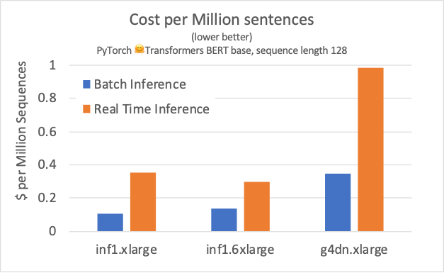
To maximize inference performance of Hugging Face models on AWS Inferentia, you use AWS Neuron PyTorch framework integration. Neuron is a software development kit (SDK) that integrates with popular ML frameworks, such as TensorFlow and PyTorch, expanding the frameworks APIs so you can run high-performance inference easily and cost-effectively on Amazon EC2 Inf1 instances. With a minimal code change, you can compile and optimize your pretrained models to run on AWS Inferentia. The Neuron team is consistently releasing updates with new features and increased model performance. With the v1.13 release, the performance of transformers based models improved by an additional 10%–15%, pushing the boundaries of minimal latency and maximum throughput, even for larger NLP workloads.
To test out the Neuron SDK features yourself, check out the latest Utilizing Neuron Capabilities for PyTorch.
The NeuronCore Pipeline mode explained
Each AWS Inferentia chip, available through the Inf1 instance family, contains four NeuronCores. The different instance sizes provide 1 to 16 chips, totaling 64 NeuronCores on the largest instance size, the inf1.24xlarge. The NeuronCore is a compute unit that runs the operations of the Neural Network (NN) graph.
When you compile a model without Pipeline mode, the Neuron compiler optimizes the supported NN operations to run on a single NeuronCore. You can combine the NeuronCores into groups, even across AWS Inferentia chips, to run the compile model. This configuration allows you to use multiple NeuronCores in data parallel mode across AWS Inferentia chips. This means that, even on the smallest instance size, four models can be active at any given time. Data parallel implementation of four (or more) models provides the highest throughput and lowest cost in most cases. This performance boost comes with minimum impact on latency, because AWS Inferentia is optimized to maximize throughput at small batch sizes.
With Pipeline mode, the Neuron compiler optimizes the partitioning and placement of a single NN graph across a requested number of NeuronCores, in a completely automatic process. It allows for an efficient use of the hardware because the NeuronCores in the pipeline run streaming inference requests, using a faster on-chip cache to hold the model weights. When one of the cores in the pipeline finishes processing a first request it can start processing following requests, without waiting for the last core to complete processing the first request. This streaming pipeline inference increases per core hardware utilization, even when running inference of small batch sizes on real-time applications, such as batch size 1.
Finding the optimum number of NeuronCores to fit a single large model is an empirical process. A good starting point is to use the following approximate formula, but we recommend experimenting with multiple configurations to achieve an optimum deployment:
neuronCore_pipeline_cores = 4*round(number-of-weights-in-model/(2E7))
The compiler directly takes the value of neuroncore-pipeline-cores compilation flag, and that is all there is to it! To enable this feature, add the argument to the usual compilation flow of your desired framework.
In TensorFlow Neuron, use the following code:
import numpy as np
import tensorflow.neuron as tfn

example_input = np.zeros([1,224,224,3], dtype='float16')
tfn.saved_model.compile("<Path to your saved model>",
                        "<Path to write compiled model>/1",
                        model_feed_dict={'input_1:0' : example_input },
                        compiler_args = ['--neuroncore-pipeline-cores', '8'])
In PyTorch Neuron, use the following code:
import torch
import torch_neuron

model = torch.jit.load(<Path to your traced model>)
inputs = torch.zeros([1, 3, 224, 224], dtype=torch.float32)

model_compiled = torch.neuron.trace(model,
                           example_inputs=inputs,
                           compiler_args = ['--neuroncore-pipeline-cores', '8'])
For more information about the NeuronCore Pipeline and other Neuron features, see Neuron Features.
Run HuggingFace question answering models in AWS Inferentia
To run a Hugging Face BertForQuestionAnswering model on AWS Inferentia, you only need to add a single, extra line of code to the usual Transformers implementation, besides importing the torch_neuron framework. You can adapt the following example of the forward pass method according to the following snippet:
from transformers import BertTokenizer, BertForQuestionAnswering
import torch
import torch_neuron

tokenizer = BertTokenizer.from_pretrained('twmkn9/bert-base-uncased-squad2')
model = BertForQuestionAnswering.from_pretrained('twmkn9/bert-base-uncased-squad2',return_dict=False)

question, text = "Who was Jim Henson?", "Jim Henson was a nice puppet"
inputs = tokenizer(question, text, return_tensors='pt')

neuron_model = torch.neuron.trace(model,
                                  example_inputs = (inputs['input_ids'],inputs['attention_mask']),
                                  verbose=1)

outputs = neuron_model(*(inputs['input_ids'],inputs['attention_mask']))
The one extra line in the preceding code is the call to the torch.neuron.trace() method. This call compiles the model and returns a new neuron_model() method that you can use to run inference over the original inputs, as shown in the last line of the script. If you want to test this example, see PyTorch Hugging Face pretrained BERT Tutorial.
The ability to compile and run inference using the pretrained models—or even fine-tuned, as in the preceding code—directly from the Hugging Face model repository is the initial step towards optimizing deployments in production. This first step can already produce two times greater performance with 70% lower cost when compared to a GPU alternative (which we discuss later in this post). When you combine NeuronCore Groups and Pipelines features, you can explore many other ways of packaging the models within a single Inf1 instance.
Optimize model deployment with NeuronCore Groups and Pipelines
The HuggingFace question answering deployment requires some of the model’s parameters to be set a priori. Neuron is an ahead-of-time (AOT) compiler, which requires knowledge of the tensor shapes at compile time. For that, we define both batch size and sequence length for our model deployment. In the previous example, the Neuron framework inferred those from the example input passed on the trace call: (inputs[‘input_ids’], inputs[‘attention_mask’]).
Besides those two model parameters, you can set the compiler argument ‘--neuroncore-pipeline-cores’ and the environment variable ‘NEURONCORE_GROUP_SIZES‘ to fine-tune how your model server consumes the NeuronCores on the AWS Inferentia chip.
For example, to maximize the number of concurrent server workers processing the inference request on a single AWS Inferentia chip—four cores—you set NEURONCORE_GROUP_SIZES=”1,1,1,1” and ‘--neuroncore-pipeline-cores’ to 1, or leave it out as a compiler argument. The following image depicts this split. It’s a full data parallel deployment.
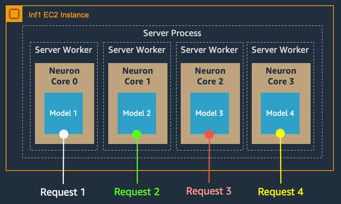
For minimum latency, you can set ‘--neuroncore-pipeline-cores’ to 4 and NEURONCORE_GROUP_SIZES=”4” so that the process consumes all four NeuronCores at once, for a single model. The AWS Inferentia chip can process four inference requests concurrently, as a stream. The model pipeline parallel deployment looks like the following figure.

Data parallel deployments favor throughput with multiple workers processing requests concurrently. The pipeline parallel, however, favors latency, but can also improve throughput due to the stream processing behavior. With these two extra parameters, you can fine-tune the serving application architecture according to the most important serving metrics for your use case.
Optimize for minimum latency: Multi-core pipeline parallel
Consider an application that requires minimum latency, such as sequence classification as part of an online chatbot workflow. As the user submits text, a model running on the backend classifies the intent of a single user input and is bounded by how fast it can infer. The model most likely has to provide responses to single input (batch size 1) requests.
The following table compare the performance and cost of Inf1 instances vs. the g4dn.xlarge—the most optimized GPU instance family for inference in the cloud—while running the HuggingFace BERT base model in a data parallel vs. pipeline parallel configuration and batch size 1. Looking at the 95th percentile (p95) of latency, we get lower values in Pipeline mode for both the 4 core inf1.xlarge and the 16 cores inf1.6xlarge instances. The best configuration between Inf1 instances is the 16 cores case, with a 58% reduction in latency, reaching 6 milliseconds.
| Instance | Batch Size | Inference Mode | NeuronCores per model | Throughput [sentences/sec] | Latency p95 [seconds] | Cost per 1M inferences | Throughput ratio [inf1/g4dn] | Cost ratio [inf1/g4dn] |
| inf1.xlarge | 1 | Data Parallel | 1 | 245 | 0.0165 | $0.42 | 1.6 | 43% |
| inf1.xlarge | 1 | Pipeline Parallel | 4 | 291 | 0.0138 | $0.35 | 2.0 | 36% |
| inf1.6xlarge | 1 | Data Parallel | 1 | 974 | 0.0166 | $0.54 | 6.5 | 55% |
| inf1.6xlarge | 1 | Pipeline Parallel | 16 | 1793 | 0.0069 | $0.30 | 12.0 | 30% |
| g4dn.xlarge | 1 | – | – | 149 | 0.0082 | $0.98 |
The model tested was the PyTorch version of HuggingFace bert-base-uncase, with sequence length 128. On AWS Inferentia, we compile the model to use all available cores and run full pipeline parallel. For the data parallel cases, we compile the models for a single core and configured the NeuronCore Groups to run a worker model per core. The GPU deployment used the same setup as AWS Inferentia, where the model was traced with TorchScript JIT and cast to mixed precision using PyTorch AMP Autocast.
Throughput also increased 1.84 times with Pipeline mode on AWS Inferentia, reaching 1,793 sentences per second, which is 12 times the throughput of g4dn.xlarge. The cost of inference on this configuration also favors the inf1.6xlarge over the most cost-effective GPU option, even at a higher cost per hour. The cost per million sentences is 70% lower based on Amazon Elastic Compute Cloud (Amazon EC2) On-Demand instance pricing. For latency sensitive applications that can’t utilize the full throughput of the inf1.6xlarge, or for smaller models such as BERT Small, we recommend using Pipeline mode on inf1.xlarge for a cost-effective deployment.
Optimize for maximum throughput: Single-core data parallel
An NLP use case that requires increase throughput over minimum latency is extractive question answering tasks, as part of a search and document retrieval pipeline. In this case, increasing the number of document sections processed in parallel can speed up the search result or improve the quality and breadth of searched answers. In such a setup, inferences are more likely to run in batches (batch size larger than 1).
To achieve maximum throughput, we found through experimentation the optimum batch size to be 6 on AWS Inferentia, for the same model tested before. On g4dn.xlarge, we ran batch 64 without running out of GPU memory. The following results help show how batch size 6 can provide 9.2 times more throughput on inf1.6xlarge at 61% lower cost, when compared to GPU.
| Instance | Batch Size | Inference Mode | NeuronCores per model | Throughput [sentences/sec] | Latency p95 [seconds] | Cost per 1M inferences | Throughput ratio [inf1/g4dn] | Cost ratio [inf1/g4dn] |
| inf1.xlarge | 6 | Data Parallel | 1 | 985 | 0.0249 | $0.10 | 2.3 | 30% |
| inf1.xlarge | 6 | Pipeline Parallel | 4 | 945 | 0.0259 | $0.11 | 2.2 | 31% |
| inf1.6xlarge | 6 | Data Parallel | 1 | 3880 | 0.0258 | $0.14 | 9.2 | 39% |
| inf1.6xlarge | 6 | Pipeline Parallel | 16 | 2302 | 0.0310 | $0.23 | 5.5 | 66% |
| g4dn.xlarge | 64 | – | – | 422 | 0.1533 | $0.35 |
In this application, cost considerations can also impact the final serving infrastructure design. The most cost-efficient way of running the batched inferences is using the inf1.xlarge instance. It achieves 2.3 times higher throughput than the GPU alternative, at 70% lower cost. Choosing between inf1.xlarge and inf1.6xlarge depends only on the main objective: minimum cost or maximum throughput.
To test out the NeuronCore Pipeline and Groups feature yourself, check out the latest Utilizing Neuron Capabilities tutorials for PyTorch.
Conclusion
In this post, we explored ways to optimize your NLP deployments using the NeuronCore Groups and Pipeline features. The native integration of AWS Neuron SDK and PyTorch allowed you to compile and optimize the HuggingFace Transformers model to run on AWS Inferentia with minimal code change. By tunning the deployment architecture to be pipeline parallel, the BERT models achieve minimum latency for real-time applications, with 12 times higher throughput than a g4dn.xlarge alternative, while costing 70% less to run. For batch inferencing, we achieve 9.2 times higher throughput at 60% less cost.
The Neuron SDK features described in this post also apply to other ML model types and frameworks. For more information, see the AWS Neuron Documentation.
Learn more about the AWS Inferentia chip and the Amazon EC2 Inf1 instances to get started running your own custom ML pipelines on AWS Inferentia using the Neuron SDK.
About the Authors
 Fabio Nonato de Paula is a Sr. Manager, Solutions Architect for Annapurna Labs at AWS. He helps customers use AWS Inferentia and the AWS Neuron SDK to accelerate and scale ML workloads in AWS. Fabio is passionate about democratizing access to accelerated ML and putting deep learning models in production. Outside of work, you can find Fabio riding his motorcycle on the hills of Livermore valley or reading ComiXology.
 Mahadevan Balasubramaniam is a Principal Solutions Architect for Autonomous Computing with nearly 20 years of experience in the area of physics infused deep learning, building and deploying digital twins for industrial systems at scale. Mahadevan obtained his PhD in Mechanical Engineering from Massachusetts Institute of Technology and has over 25 patents and publications to his credit.
Do Wide and Deep Networks Learn the Same Things?
Posted by Thao Nguyen, AI Resident, Google Research
A common practice to improve a neural network’s performance and tailor it to available computational resources is to adjust the architecture depth and width. Indeed, popular families of neural networks, including EfficientNet, ResNet and Transformers, consist of a set of architectures of flexible depths and widths. However, beyond the effect on accuracy, there is limited understanding of how these fundamental choices of architecture design affect the model, such as the impact on its internal representations.
In “Do Wide and Deep Networks Learn the Same Things? Uncovering How Neural Network Representations Vary with Width and Depth”, we perform a systematic study of the similarity between wide and deep networks from the same architectural family through the lens of their hidden representations and final outputs. In very wide or very deep models, we find a characteristic block structure in their internal representations, and establish a connection between this phenomenon and model overparameterization. Comparisons across models demonstrate that those without the block structure show significant similarity between representations in corresponding layers, but those containing the block structure exhibit highly dissimilar representations. These properties of the internal representations in turn translate to systematically different errors at the class and example levels for wide and deep models when they are evaluated on the same test set.
Comparing Representation Similarity with CKA
We extended prior work on analyzing representations by leveraging our previously developed Centered Kernel Alignment (CKA) technique, which provides a robust, scalable way to determine the similarity between the representations learned by any pair of neural network layers. CKA takes as input the representations (i.e., the activation matrices) from two layers, and outputs a similarity score between 0 (not at all similar) and 1 (identical representations).
We apply CKA to a family of ResNets of varying depths and widths, trained on common benchmark datasets (CIFAR-10, CIFAR-100 and ImageNet), and use representation heatmaps to illustrate the results. The x and y axes of each heatmap index the layers of the model(s) in consideration, going from input to output, and each entry (i, j) is the CKA similarity score between layer i and layer j.
 |
| We use CKA to compute the representation similarity for all pairs of layers within a single model (i.e., when network 1 and network 2 are identical), and across models (i.e., when network 1 and network 2 are trained with different random initializations, or have different architectures altogether). |
Below is an example of the resulting heatmap when we compare representations of each layer to every other layer within a single ResNet of depth 26 and width multiplier 1. In the design convention used here, the stated depth only refers to the number of convolutional layers in the network, but we analyze all layers present, and the width multiplier applies to the number of filters in each convolution. Notice the checkerboard pattern in the heatmap, which is caused by skip connections (shortcuts between layers) in the architecture.

The Emergence of the Block Structure
What stands out from the representation heatmaps of deeper or wider networks is the emergence of a large set of consecutive layers with highly similar representations, which appears in the heatmaps as a yellow square (i.e., a region with high CKA scores). This phenomenon, which we call the block structure, suggests that the underlying layers may not be as efficient at progressively refining the network’s representations as we expect. Indeed, we show that the task performance becomes stagnant inside the block structure, and that it is possible to prune some underlying layers without affecting the final performance.
 |
| Block structure — a large, contiguous set of layers with highly similar representations — emerges with increasing width or depth. Each heatmap panel shows the CKA similarity between all pairs of layers within a single neural network. While its size and position can vary across different training runs, the block structure is a robust phenomenon that arises consistently in larger models. |
With additional experiments, we show that the block structure has less to do with the absolute model size, than with the size of the model relative to the size of the training dataset. As we reduce the training dataset size, the block structure starts to appear in shallower and narrower networks:
 |
| With increasing network width (towards the right along each row) and decreasing dataset size (down each column), the relative model capacity (with respect to a given task) is effectively inflated, and the block structure begins to appear in smaller models. |
Through further analysis, we are also able to demonstrate that the block structure arises from preserving and propagating the dominant principal components of its underlying representations. Refer to our paper for more details.
Comparing Representations Across Models
Going further, we study the implications of depth and width on representations across models of different random initializations and different architectures, and find that the presence of block structure makes a significant difference in this context as well. Despite having different architectures, wide and deep models without the block structure do exhibit representation similarity with each other, with corresponding layers broadly being of the same proportional depth in the model. However, when the block structure is present, its representations are unique to each model. This suggests that despite having similar overall performance, each wide or deep model with the block structure picks up a unique mapping from the input to the output.
 |
| For smaller models (e.g., ResNet-38 1×), CKA across different initializations (off the diagonal) closely resembles CKA within a single model (on the diagonal). In contrast, representations within the block structure of wider and deeper models (e.g., ResNet-38 10×, ResNet-164 1×) are highly dissimilar across training runs. |
Error Analysis of Wide and Deep Models
Having explored the properties of the learned representations of wide and deep models, we next turn to understanding how they influence the diversity of the output predictions. We train populations of networks of different architectures and determine on which test set examples each architecture configuration tends to make errors.
On both CIFAR-10 and ImageNet datasets, wide and deep models that have the same average accuracy still demonstrate statistically significant differences in example-level predictions. The same observation holds for class-level errors on ImageNet, with wide models exhibiting a small advantage in identifying classes corresponding to scenes, and deep networks being relatively more accurate on consumer goods.
 |
| Per-class differences on ImageNet between models with increased width (y-axis) or depth (x-axis). Orange dots reflect differences between two sets of 50 different random initializations of ResNet-83 (1×). |
Conclusions
In studying the effects of depth and width on internal representations, we uncover a block structure phenomenon, and demonstrate its connection to model capacity. We also show that wide and deep models exhibit systematic output differences at class and example levels. Check out the paper for full details on these results and additional insights! We’re excited about the many interesting open questions these findings suggest, such as how the block structure arises during training, whether the phenomenon occurs in domains beyond image classification, and ways these insights on internal representations can inform model efficiency and generalization.
Acknowledgements
This is a joint work with Maithra Raghu and Simon Kornblith. We would like to thank Tom Small for the visualizations of the representation heatmap.