Posted by Nachiappan Valliappan, Senior Software Engineer and Kai Kohlhoff, Staff Research Scientist, Google Research
Eye movement has been studied widely across vision science, language, and usability since the 1970s. Beyond basic research, a better understanding of eye movement could be useful in a wide variety of applications, ranging across usability and user experience research, gaming, driving, and gaze-based interaction for accessibility to healthcare. However, progress has been limited because most prior research has focused on specialized hardware-based eye trackers that are expensive and do not easily scale.
In “Accelerating eye movement research via accurate and affordable smartphone eye tracking”, published in Nature Communications, and “Digital biomarker of mental fatigue”, published in npj Digital Medicine, we present accurate, smartphone-based, ML-powered eye tracking that has the potential to unlock new research into applications across the fields of vision, accessibility, healthcare, and wellness, while additionally providing orders-of-magnitude scaling across diverse populations in the world, all using the front-facing camera on a smartphone. We also discuss the potential use of this technology as a digital biomarker of mental fatigue, which can be useful for improved wellness.
Model Overview The core of our gaze model was a multilayer feed-forward convolutional neural network (ConvNet) trained on the MIT GazeCapture dataset. A face detection algorithm selected the face region with associated eye corner landmarks, which were used to crop the images down to the eye region alone. These cropped frames were fed through two identical ConvNet towers with shared weights. Each convolutional layer was followed by an average pooling layer. Eye corner landmarks were combined with the output of the two towers through fully connected layers. Rectified Linear Units (ReLUs) were used for all layers except the final fully connected output layer (FC6), which had no activation.
Architecture of the unpersonalized gaze model. Eye regions, extracted from a front-facing camera image, serve as input into a convolutional neural network. Fully-connected (FC) layers combine the output with eye corner landmarks to infer gaze x– and y-locations on screen via a multi-regression output layer.
The unpersonalized gaze model accuracy was improved by fine-tuning and per-participant personalization. For the latter, a lightweight regression model was fitted to the model’s penultimate ReLU layer and participant-specific data.
Model Evaluation To evaluate the model, we collected data from consenting study participants as they viewed dots that appeared at random locations on a blank screen. The model error was computed as the distance (in cm) between the stimulus location and model prediction. Results show that while the unpersonalized model has high error, personalization with ~30s of calibration data led to an over fourfold error reduction (from 1.92 to 0.46cm). At a viewing distance of 25-40 cm, this corresponds to 0.6-1° accuracy, a significant improvement over the 2.4-3° reported in previous work [1, 2].
Additional experiments show that the smartphone eye tracker model’s accuracy is comparable to state-of-the-art wearable eye trackers both when the phone is placed on a device stand, as well as when users hold the phone freely in their hand in a near frontal headpose. In contrast to specialized eye tracking hardware with multiple infrared cameras close to each eye, running our gaze model using a smartphone’s single front-facing RGB camera is significantly more cost effective (~100x cheaper) and scalable.
Using this smartphone technology, we were able to replicate key findings from prior eye movement research in neuroscience and psychology, including standard oculomotor tasks (to understand basic visual functioning in the brain) and natural image understanding. For example, in a simple prosaccade task, which tests a person’s ability to quickly move their eyes towards a stimulus that appears on the screen, we found that the average saccade latency (time to move the eyes) matches prior work for basic visual health (210ms versus 200-250ms). In controlled visual search tasks, we were able to replicate key findings, such as the effect of target saliency and clutter on eye movements.
Example gaze scanpaths show the effect of the target’s saliency (i.e., color contrast) on visual search performance. Fewer fixations are required to find a target (left) with high saliency (different from the distractors), while more fixations are required to find a target (right) with low saliency (similar to the distractors).
For complex stimuli, such as natural images, we found that the gaze distribution (computed by aggregating gaze positions across all participants) from our smartphone eye tracker are similar to those obtained from bulky, expensive eye trackers that used highly controlled settings, such as laboratory chin rest systems. While the smartphone-based gaze heatmaps have a broader distribution (i.e., they appear more “blurred”) than hardware-based eye trackers, they are highly correlated both at the pixel level (r = 0.74) and object level (r = 0.90). These results suggest that this technology could be used to scale gaze analysis for complex stimuli such as natural and medical images (e.g., radiologists viewing MRI/PET scans).
Similar gaze distribution from our smartphone approach vs. a more expensive (100x) eye tracker (from the OSIE dataset).
We found that smartphone gaze could also help detect difficulty with reading comprehension. Participants reading passages spent significantly more time looking within the relevant excerpts when they answered correctly. However, as comprehension difficulty increased, they spent more time looking at the irrelevant excerpts in the passage before finding the relevant excerpt that contained the answer. The fraction of gaze time spent on the relevant excerpt was a good predictor of comprehension, and strongly negatively correlated with comprehension difficulty (r = −0.72).
Digital Biomarker of Mental Fatigue Gaze detection is an important tool to detect alertness and wellbeing, and is studied widely in medicine, sleep research, and mission-critical settings such as medical surgeries, aviation safety, etc. However, existing fatigue tests are subjective and often time-consuming. In our recent paper published in npj Digital Medicine, we demonstrated that smartphone gaze is significantly impaired with mental fatigue, and can be used to track the onset and progression of fatigue.
A simple model predicts mental fatigue reliably using just a few minutes of gaze data from participants performing a task. We validated these findings in two different experiments — using a language-independent object-tracking task and a language-dependent proofreading task. As shown below, in the object-tracking task, participants’ gaze initially follows the object’s circular trajectory, but under fatigue, their gaze shows high errors and deviations. Given the pervasiveness of phones, these results suggest that smartphone-based gaze could provide a scalable, digital biomarker of mental fatigue.
Example gaze scanpaths for a participant with no fatigue (left) versus with mental fatigue (right) as they track an object following a circular trajectory.
The corresponding progression of fatigue scores (ground truth) and model prediction as a function of time on task.
Beyond wellness, smartphone gaze could also provide a digital phenotype for screening or monitoring health conditions such as autism spectrum disorder, dyslexia, concussion and more. This could enable timely and early interventions, especially for countries with limited access to healthcare services.
Another area that could benefit tremendously is accessibility. People with conditions such as ALS, locked-in syndrome and stroke have impaired speech and motor ability. Smartphone gaze could provide a powerful way to make daily tasks easier by using gaze for interaction, as recently demonstrated with Look to Speak.
Ethical Considerations Gaze research needs careful consideration, including being mindful of the correct use of such technology — applications should obtain explicit approval and fully informed consent from users for the specific task at hand. In our work, all data was collected for research purposes with users’ explicit approval and consent. In addition, users were allowed to opt out at any point and request their data to be deleted. We continue to research additional ways to ensure ML fairness and improve the accuracy and robustness of gaze technology across demographics, in a responsible, privacy-preserving way.
Conclusion Our findings of accurate and affordable ML-powered smartphone eye tracking offer the potential for orders-of-magnitude scaling of eye movement research across disciplines (e.g., neuroscience, psychology and human-computer interaction). They unlock potential new applications for societal good, such as gaze-based interaction for accessibility, and smartphone-based screening and monitoring tools for wellness and healthcare.
Acknowledgements This work involved collaborative efforts from a multidisciplinary team of software engineers, researchers, and cross-functional contributors. We’d like to thank all the co-authors of the papers, including our team members, Junfeng He, Na Dai, Pingmei Xu, Venky Ramachandran; interns, Ethan Steinberg, Kantwon Rogers, Li Guo, and Vincent Tseng; collaborators, Tanzeem Choudhury; and UXRs: Mina Shojaeizadeh, Preeti Talwai, and Ran Tao. We’d also like to thank Tomer Shekel, Gaurav Nemade, and Reena Lee for their contributions to this project, and Vidhya Navalpakkam for her technical leadership in initiating and overseeing this body of work.
A common problem in manufacturing is verifying that products meet quality standards. You can use manual inspection on a subset of the products, but it’s usually not scalable enough to meet demand as production grows. In this post, I go through the steps of creating an end-to-end machine vision solution that identifies visual anomalies in products using Amazon Lookout for Vision. I’ll show you how to train a model that performs anomaly detection, use the model in real-time, update the model when new data is available, and how to monitor the model.
Solution overview
Imagine a factory producing Lego bricks. The bricks are transported on a conveyor belt in front of a camera that determines if they meet the factory’s quality standards. When a brick on the belt breaks a light beam, the device takes a photo and sends it to Amazon Lookout for Vision for anomaly detection. If a defective brick is identified, it’s pushed off the belt by a pusher.
The following diagram illustrates the architecture of our anomaly detection solution, which uses Amazon Lookout for Vision, Amazon Simple Storage Service (Amazon S3), and a Raspberry Pi.
Amazon Lookout for Vision is a machine learning (ML) service that uses machine vision to help you identify visual defects in products without needing any ML experience. It uses deep learning to remove the need for carefully calibrated environments in terms of lighting and camera angle, which many existing machine vision techniques require.
To get started with Amazon Lookout for Vision, you need to provide data for the service to use when training the underlying deep learning models. The dataset used in this post consists of 289 normal and 116 anomalous images of a Lego brick, which are hosted in an S3 bucket that I have made public so you can download the dataset.
To make the scenario more realistic, I’ve varied the lighting and camera position between images. Additionally, I use 20 test images and 9 new images to update the model later on with both normal and anomalous images. The anomalous images were created by drawing on and scratching the brick, changing the brick color, adding other bricks, and breaking off small pieces to simulate production defects. The following image shows the physical setup used when collecting training images.
Pre-requisites
To follow along with this post, you’ll need the following:
An AWS account to train and use Amazon Lookout for Vision
A camera (for this post, I use a Pi camera)
A device that can run code (I use a Raspberry Pi 4)
Train the model
To use the dataset when training a model, you first upload the training data to Amazon S3 and create an Amazon Lookout for Vision project. A project is an abstraction around the training dataset and multiple model versions. You can think of a project as a collection of the resources that relate to a specific machine vision use case. For instance, in this post, I use one dataset but create multiple model versions as I gradually optimize the model for the use case with new data, all within the boundaries of one project.
You can use the SDK, AWS Command Line Interface (AWS CLI), and AWS Management Console to perform all the steps required to create and train a model. For this post, I use a combination of the AWS CLI and the console to train and start the model, and use the SDK to send images for anomaly detection from the Raspberry Pi.
To train the model, we complete the following high-level steps:
Upload the training data to Amazon S3.
Create an Amazon Lookout for Vision project.
Create an Amazon Lookout for Vision dataset.
Train the model.
Upload the training data to Amazon S3
To get started, complete the following steps:
Download the dataset to your computer.
Create an S3 bucket and upload the training data.
I named my bucket l4vdemo, but bucket names need to be globally unique, so make sure to change it if you copy the following code. Make sure to keep the folder structure in the dataset, because Amazon Lookout for Vision uses it to label normal and anomalous images automatically based on folder name. You could use the integrated labeling tool on the Amazon Lookout for Vision console or Amazon SageMaker Ground Truth to label the data, but the automatic labeler allows you to keep the folder structure and save some time.
On the Amazon Lookout for Vision console, choose Projects in the navigation pane.
Choose Create project.
For Project name, enter a name.
Choose Create project.
Create the dataset
For this post, I create a single dataset and import the training data from the S3 bucket I uploaded the data to in Step 1.
Choose Create dataset.
Select import images from S3 bucket.
For S3 URI, enter the URI for your bucket (for this post, s3://l4vdemo/, but make sure to use the unique bucket name you created).
For Automatic labeling, select Automatically attach labels to images based on the folder name.
This allows you to use the existing folder structure to infer whether your images are normal or anomalous.
Choose Create dataset.
Train the model
After we create the dataset, the number of labeled and unlabeled images should be visible in the Filters pane, as well as the number of normal and anomalous images.
To start training a deep learning model, choose Train model.
Model training can take a few hours depending on the number of images in the training dataset.
When training is complete, in the navigation pane, chose Models under your project.
You should see the newly created model listed with a status of Training complete.
Choose the model to see performance metrics like precision, recall and F1 score, training duration, and more model metadata.
Use the model
Now that a model is trained, let’s test it on data it hasn’t seen before. To use the model, you must first start hosting it to provision all backend resources required to perform real-time inference.
When starting the model hosting, you pass both project name and model version as arguments to identify the model. You also need to specify the number of inference units to use; each unit enables approximately five requests per second.
To use the hosted model, use the detect-anomalies command and pass in the project and model version along with the image to perform inference on:
The flag IsAnomalous is true and Amazon Lookout for Vision also provides a confidence score that tells you how sure the model is of its classification. The service always provides a binary classification, but you can use the confidence score to make more well-informed decisions, such as whether to scrap the brick directly or send it for manual inspection. You could also persist images with lower confidence scores and use them to update the model, which I show you how to do in the next section.
Keep in mind that you’re charged for the model as long as it’s running, so stop it when you no longer need it:
As new data becomes available, you may want to maintain or update the model to accommodate for new types of defects and increase the model’s overall performance. The dataset contains nine images in the new-data folder, which I use to update the model. To update an Amazon Lookout for Vision model, you run a trial detection and verify the machine predictions to correct the model predictions, and add the verified images to your training dataset.
Run a trial detection
To run a trial detection, complete the following steps:
On the Amazon Lookout for Vision console, under your model in the navigation pane, choose Trial detections.
Choose Run trial detection.
For Trial name, enter a name.
For Import images, select Import images from S3 bucket.
For S3 URI, enter the URI of the new-data folder that you uploaded in Step 1 of training the model
Choose Run trial
Verify machine predictions
When the trial detection is complete, you can verify the machine predictions.
Choose Verify machine predictions.
Select either Correct or Incorrect to label the images
When all the images have been labeled, choose Add verified images to dataset.
This updates your training dataset with the new data.
Retrain the model
After you update your training dataset with the new data, you can see that the number of labeled images in your dataset has increased, along with the number of verified images.
Choose Train model to train a new version of the model.
When the new model is training, on the Models page, you can verify that a new model version is being trained. When the training is complete, you can view model performance metrics on the Models page and start using the new version.
Anomaly detection application
Now that I’ve trained my model, let’s use it with the Raspberry Pi to sort Lego bricks. In this use case, I’ve set up a Raspberry Pi with a camera that gets triggered whenever a break beam sensor senses a Lego brick. We use the following code:
import boto3
from picamera import PiCamera
import my_break_bream_sensor
import my_pusher

l4v_client = boto3.client('lookoutvision')
image_path = '/home/pi/Desktop/my_image.jpg'

with PiCamera() as camera:
    while(True):
        if my_break_bream_sensor.isBroken():  # Replace with your own sensor.
            camera.capture(image_path)
            with open(image_path, 'rb') as image:
                response = l4v_client.detect_anomalies(ProjectName='lego-demo',
                                                       ContentType='image/jpeg',
                                                       Body=image.read(),
                                                       ModelVersion='2')

            is_anomalous = response['DetectAnomalyResult']['IsAnomalous']
            if (is_anomalous):
                my_pusher.push()  # Replace with your own pusher.
Monitoring the model
When the system is up and running, you can use the Amazon Lookout for Vision dashboard to visualize metadata from the projects you have running, such as the number of detected anomalies during a specific time period. The dashboard provides an overview of all current projects, as well as aggregated information like total anomaly ratio.
Pricing
The cost of the solution is based on the time to train the model and the time the model is running. You can divide the cost across all analyzed products to get a per-product cost. Assuming one brick is analyzed per second nonstop for a month, the cost of the solution, excluding hardware and training, is around $0.001 per brick, assuming we’re using 1 inference unit. However, if you increase production speed and analyze five bricks per second, the cost is around $0.0002 per brick.
Conclusion
Now you know how to use Amazon Lookout for Vision to train, run, update, and monitor an anomaly detection application. The use case in this post is of course simplified; you will have other requirements specific to your needs. Many factors affect the total end-to-end latency when performing inference on an image. The Amazon Lookout for Vision model runs in the cloud, which means that you need to evaluate and test network availability and bandwidth to ensure that the requirements can be met. To avoid creating bottlenecks, you can use a circuit breaker in your application to manage timeouts and prevent congestion in case of network issues.
Now that you know how to train, test and use and update an ML model for anomaly detection, try it out with your own data! To get further details about Amazon Lookout for Vision, please visit the webpage!
About the Authors
Niklas Palm is a Solutions Architect at AWS in Stockholm, Sweden, where he helps customers across the Nordics succeed in the cloud. He’s particularly passionate about serverless technologies along with IoT and machine learning. Outside of work, Niklas is an avid cross-country skier and snowboarder as well as a master egg boiler.
Early on, Giovanni Paolini knew little about machine learning — now he’s leading new science on artificial intelligence that could inform AWS products.Read More
Knowledge Graphs (KGs) have emerged as a compelling abstraction for organizing the world’s structured knowledge, and as a way to integrate information extracted from multiple data sources. Knowledge graphs have started to play a central role in representing the information extracted using natural language processing and computer vision. Domain knowledge expressed in KGs is being input into machine learning models to produce better predictions. Our goals in this blog post are to (a) explain the basic terminology, concepts, and usage of KGs, (b) highlight recent applications of KGs that have led to a surge in their popularity, and (c) situate KGs in the overall landscape of AI. This blog post is a good starting point before reading a more extensive survey or following research seminars on this topic.
Knowledge Graph Definition
A directed labeled graph is a 4-tuple G = (N, E, L, f), where N is a set of nodes, E ⊆ N × N is a set of edges, L is a set of labels, and f: E→L, is an assignment function from edges to labels. An assignment of a label B to an edge E=(A,C) can be viewed as a triple (A, B, C) and visualized as shown in Figure 1.
A knowledge graph is a directed labeled graph in which we have associated domain specific meanings with nodes and edges. Anything can act as a node, for example, people, company, computer, etc. An edge label captures the relationship of interest between the nodes, for example, a friendship relationship between two people, a customer relationship between a company and person, or a network connection between two computers, etc.
The directed labeled graph representation is used in a variety of ways depending on the needs of an application. A directed labeled graph such as the one in which the nodes are people, and the edges capture the parent relationship is also known as a data graph. A directed labeled graph in which the nodes are classes of objects (e.g., Book, Textbook, etc.), and the edges capture the subclass relationship, is also known as a taxonomy. In some data models, given a triple (A,B,C), we refer to A, B, C as the subject, the predicate, and the object of the triple respectively.
A knowledge graph serves as a data structure in which an application stores information. The information could be added to the knowledge graph through a combination of human input, automated and semi-automated methods. Regardless of the method of knowledge entry, it is expected that the recorded information can be easily understood and verified by humans.
Many interesting computations over a graph can be reduced to navigating it. For example, in a friendship KG, to calculate the friends of friends of a person A, we can navigate the graph from A to all nodes B connected to it by a relation labeled as friend, and then recursively to all nodes C connected by the friend relation to each B.
Recent Applications of Knowledge Graphs
Use of directed labeled graphs as a data structure for storing information, and the use of graph algorithms to manipulate that information is not new. Within computer science, there have been many uses of a directed graph representation, for example, data flow graphs, binary decision diagrams, state charts, etc. We consider here two concrete applications that have led to a recent surge in the popularity of knowledge graphs: organizing information over the internet and data integration in enterprises. While discussing these applications, we also highlight what is new and different in the use of knowledge graphs.
Organizing Knowledge over the Internet
Consider the Google search for “Winterthur Zurich” which returns the result shown in the left panel of Figure 2 and a relevant portion from Wikipedia in the panel on the right. The portion of the Wikipedia page shown in the panel on the right is also known as an Infobox.
Figure 2: An example use of a knowledge graph in the results of a web search
As part of the search results, we see facts such as Winterthur is in the country Switzerland, its elevation is 430 meters, etc. This information is directly extracted from the Infoboxes from the Wikipedia page for Winterthur. Some of the data in the Wikipedia Infoboxes is populated by querying a KG called Wikidata. The data from a KG can enhance the web search in even deeper ways than illustrated in the above example, as we next discuss.
The Wikipedia page for Winterthur lists its twin towns: two are in Switzerland, one in Czech Republic, and one in Austria. The city of Ontario in California that has a Wikipedia page titled, Ontario, California, lists Winterthur as its sister city. Sister city and twin city relationships are identical as well as reciprocal. Thus, if a city A is a sister (twin) city of another city B, then B must be a sister (twin) city of A. As “Sister cities” and “Twin towns” are section headings in Wikipedia, with no definition or relationship specified between the two, it is difficult to detect this discrepancy. In contrast, in the Wikidata representation of Winterthur, there is a relationship called twinned administrative body that lists the city of Ontario. As this relationship is defined to be a symmetric relationship in the KG, the Wikidata page for the city of Ontario automatically includes Winterthur. Wikidata solves the problem of identifying equivalent relationships through the effort of its curators, and by using a KG as a storage and inference mechanism. To the degree the Wikidata KG is fully integrated into Wikipedia, the discrepancies of missing links considered in the example considered here will naturally disappear. We can visualize the two way relationship between Winterthur and Ontario in Figure 3. The KG in Figure 3 also shows other objects to which Winterthur and Ontario are connected.
Figure 3: A fragment of the Wikidata knowledge graph
Wikidata includes data from several independent providers such as the Library of Congress. By using the Wikidata identifier for Winterthur, the information released by the Library of Congress can be easily linked with other information about Winterthur present in Wikidata. Wikidata makes it easy to establish such links by publishing the definitions of relationships used in it in Schema.Org.
A well-documented list of relations in Schema.Org, also known as the relation vocabulary, gives us, at least, two advantages. First, it is easier to write queries that span across multiple datasets because queries can be framed using relations that are common to those sources. Without the usage of such common relationships across multiple sources, we would need to determine semantic relationships between them and provide appropriate translations. One example of a query that goes across multiple sources is: Display on a map the birth cities of people who died in Winterthour? Second, search engines can use such queries to retrieve information from the KG and display the query results as shown in Figure 2. Use of structured information returned in the search results is now a standard feature for the leading search engines.
A recent version of Wikidata had over 90 million objects, with over one billion relationships among those objects. Wikidata makes connections across over 4872 different catalogs in 414 different languages published by independent data providers. As per a recent estimate, 31% of the websites, and over 12 million data providers are currently using the vocabulary of Schema.Org to publish annotations to their web pages.
What is particularly new and exciting about the Wikidata knowledge graph? First, it is a graph of unprecedented scale, and is one of the largest knowledge graphs available today. Second, even though Wikidata is manually curated, the cost of curation is shared by a community of contributors. Third, some of the data in Wikidata may come from automatically extracted information, but it must be easily understood and verified as per the Wikidata editorial policies. Fourth, there is an explicit effort to provide semantic definitions of different relation names through the vocabulary in Schema.Org. Finally, the primary driving use case for Wikidata is to improve the web search. Even though Wikidata has several applications using it for analysis and visualization, its use over the web continues to be the most compelling and easily understood application.
Data Integration in Enterprises
Figure 4: 360-degree view of a customer is created by integrating external data with internal company information
Many financial institutions are interested in better managing their customer relationships through a 360-degree view, i.e., a view that integrates external information about a customer with internal information about the same customer. For example, one can integrate publicly available information from financial news, commercially sourced and curated data about supply chain relationships with internal customer information to create such a 360-degree view. To understand how such a view is useful, let us consider an example scenario. Financial news reports that “Acma Retail Inc’’ has filed for bankruptcy due to the pandemic, because of which many of its suppliers will face financial stress. Such stress can pass deep down into its supply chain and trigger financial difficulties for other clients. For example, if a company A who is a supplier for Acma is undergoing financial stress, a similar stress will be experienced by companies who are suppliers of A. Such supply chain relationships are curated as part of a commercially available dataset called Factset. In a 360-degree view, the data from Factset and the financial news are integrated with the internal customer databases. The resulting KG accurately tracks Acma supply chain, identifies stressed suppliers with different revenue exposure, and identifies companies whose risk may be worth monitoring.
To create the 360-degree view of a customer, the data integration process begins with business analysts sketching out a schema of the key entities, events and the relationships they are interested in tracking. The visual nature of the KG schemas makes it easier for the business experts to engage and specify their requirements. The data from the individual sources is then loaded into a knowledge graph engine. The storage format of triples allows us to translate only those relationships that are of immediate relevance to the schema defined by the business domain experts. Rest of the data can still be loaded as triples but does not require us to incur the upfront cost of relating them into the defined schema. As the KGs use a generic schema of triples, changing requirements during the analysis process are easier to incorporate. Finally, the storage format mirrors the schema that the domain experts define.
What is particularly new and exciting about the use of knowledge graphs for data integration? First, a generic schema of triples substantially reduces the cost of starting with a data integration project. Second, it is much easier to adapt a triple-based schema in response to changes than the comparable effort required to adapt a traditional relational database. Third, and finally, modern KG engines are highly optimized for answering questions that require traversing the graph relationships in the data. For the example schema of Figure 5, a graph engine has built in operations to identify the central suppliers in a supply chain network, closely related groups of customers or suppliers, and spheres of influence of different suppliers. All of these computations leverage domain-independent graph algorithms such as centrality detection and community detection. Because of ease of creating and visualizing the schema, and the built in analytics operations, KGs are becoming a popular solution for turning data into intelligence.
Knowledge Graphs in Artificial Intelligence
AI agents maintain representations of the real world and use them for reasoning. Coming up with a good representation is a problem central to AI as it allows an agent to store information and derive new conclusions from it. We begin this section by a quick review of the previous work on knowledge representation in AI, situate KGs within that context, and then provide more details about how the modern AI algorithms use KGs to store their output as well as consume them to incorporate domain knowledge.
A widely known application of approaches that originated from semantic networks is in capturing ontologies. An ontology is a formal specification of the relationships that are used in a knowledge graph. For example, in Figure 3, the concepts such as City, Country, etc. and relationships such as part of, same as, etc, and their formal definitions constitute an ontology. Using this ontology, we can draw inferences such as Winterthur is located in Switzerland.
The prior work on knowledge representation in AI that we have just reviewed has been driven in a top-down manner, that is, we first develop a model of the world, and then use reasoning algorithms to draw conclusions from them. Currently, there is a surge of activity on bottom up approaches to AI, that is, developing algorithms that can process the data from which algorithms can draw conclusions and insights. For the rest of the section, we will discuss the role KGs are playing both in storing the learned knowledge, and in providing a source of domain knowledge input to the AI algorithms.
Knowledge Graphs as the output of Machine Learning
Even though Wikidata has had success in engaging a community of volunteer curators, manual creation of knowledge graphs is, in general, expensive. Therefore, any automation we can achieve for creating a knowledge graph is highly desired. Until a few years ago, both natural language processing (NLP) and computer vision (CV) algorithms were struggling to do well on entity recognition from text and object detection from images. Because of recent progress, these algorithms are starting to move beyond the basic recognition tasks to extracting relationships among objects necessitating a representation in which the extracted relations could be stored for further processing and reasoning. We will now discuss how the automation possible through NLP and CV techniques is facilitating the creation of knowledge graphs.
Entity extraction and relation extraction from text are two fundamental tasks in NLP. Methods for performing entity and relation extraction include rule-based methods, and machine learning. The rule-based approaches leverage the syntactical structure of the sentence or specify how entities or relationships could be identified in the input text. The machine learning approaches leverage sequence labeling algorithms or language models for both entity and relation extraction.
The extracted information from multiple portions of the text needs to be correlated, and knowledge graphs provide a natural medium to accomplish such a goal. For example, from the sentence shown in Figure 6, we can extract the entities Albert Einstein, Germany, Theoretical Physicist, and Theory of Relativity; and the relations born in, occupation and developed. Once this snippet of knowledge is incorporated into a larger KG, we can use logical inference to get additional links (shown by dotted edges) such as a Theoretical Physicist is a kind of Physicist who practices Physics, and that Theory of Relativity is a branch of Physics.
A holy grail of computer vision is the complete understanding of an image, that is, detecting objects, describing their attributes, and recognizing their relationships. Understanding images would enable important applications such as image search, question answering, and robotic interactions. Much progress has been made in recent years towards this goal, including image classification and object detection. Computer vision algorithms make heavy use of machine learning methods such as classification, clustering, nearest neighbors, and the deep learning methods such as recurrent neural networks.
From the image shown in Figure 7, an image understanding system should produce a KG shown to the right. The nodes in the knowledge graph are the outputs of an object detector. Current research in computer vision focuses on developing techniques that can correctly infer the relationships between the objects, such as, man holding a bucket, and horse feeding from the bucket, etc. The KG shown to the right is an example of a knowledge graph which provides foundation for visual question answering.
Knowledge Graphs as input to Machine Learning
Machine learning algorithms can perform better if they can incorporate domain knowledge. KGs are a useful data structure for capturing domain knowledge, but machine learning algorithms require that any symbolic or discrete structure, such as a graph, should first be converted into a numerical form. We can convert symbolic inputs into a numerical form using a technique known as embeddings. To illustrate this, we will consider word embeddings and graph embeddings.
Word embeddings were originally developed for calculating similarity between words. To understand the word embeddings, we consider the following set of sentences.
I like knowledge graphs.
I like databases.
I enjoy running.
In the above set of sentences, we count how often a word appears next to another word and record the counts in a matrix. For example, the word I appears next to the word like twice, and next to the word enjoy once, and therefore, its counts for these two words are 2 and 1 respectively, and 0 for every other word. We can calculate the counts for the other words in a similar manner as shown in Table 1. Such a matrix is often referred to as word co-occurrence counts. The meaning of each word is captured by the vector in the row corresponding to that word. To calculate similarity between words, we calculate the similarity between the vectors corresponding to them. In practice, we are interested in text that may contain millions of words, and a more compact representation is desired. As the co-occurrence matrix is sparse, we can use techniques from Linear Algebra (e.g., singular value decomposition) to reduce its dimensions. The resulting vector corresponding to a word is known as its word embedding. Typical word embeddings in use today rely on vectors of length 200.
counts
I
like
enjoy
Knowledge
graphs
database
running
.
I
0
2
1
0
0
0
0
0
like
2
0
0
1
0
1
0
0
enjoy
1
0
0
0
0
0
1
0
knowledge
0
1
0
0
1
0
0
0
graphs
0
0
0
1
0
0
0
1
databases
0
1
0
0
0
0
0
1
running
0
0
1
0
0
0
0
1
.
0
0
0
0
1
1
1
0
Table 1: Matrix of co-occurrence counts
A sentence is a sequence of words, and word embeddings calculate co-occurrences of words in it. We can generalize this idea to node embeddings for a graph in the following manner: (a) traverse the graph using a random walk giving us a path through the graph (b) obtain a set of paths through repeated traversals of the graph (c) calculate co-occurrences of nodes on these paths just like we calculated co-occurrences of words in a sentence (d) each row in the matrix of co-occurrence counts give us a vector for the node corresponding to it (e) use suitable dimensionality reduction techniques to obtain a smaller vector which is referred to as a node embedding.
We can encode the whole graph into a vector which is known as its graph embedding. There are many approaches to calculate graph embeddings, but perhaps, the simplest approach is to add the vectors representing node embeddings for each of the nodes in the graph to obtain a vector representing the whole graph.
We used the example of word embeddings as precursor to explaining graph embeddings primarily for pedagogical purposes. Indeed, both have similar objectives: while word embeddings capture the meaning of words and help calculate similarity between them, node embeddings capture the meaning of nodes in a graph and help calculate similarity between them. There is also a great deal of similarity between the methods used for calculating them.
Word embeddings and graph embeddings are a way to give a symbolic input to a machine learning algorithm. A common application of word embeddings is to learn a language model that can predict what word is likely to appear next in a sequence of words. A more advanced application of word embeddings is to use them with a KG – for example, the embedding for a more frequent word could be reused for a less frequent word as long as the knowledge graph encodes that the less frequent word is its hyponym. A straightforward use for the graph embeddings calculated from a friendship graph is to recommend new friends. A more advanced use of graph embedding involves link prediction, for example, in a company graph, we can use link prediction to identify potential new customers.
Summary
A directed labeled graph is a fundamental construct in discrete mathematics, and has applications in all areas of computer science. Most notable uses of directed labeled graphs in AI and databases have taken the form of data graphs, taxonomies and ontologies. Traditionally, such applications have been small and have been created by a top down design and through manual knowledge engineering.
Distinguishing characteristics of the modern knowledge graphs from the classical knowledge graphs are: scale, bottom up development and multiple modes of construction. The early semantic networks in AI never reached the size and scale of the knowledge graphs that we see today. Difficulty in coming up with a top down schema design for data integration and the data driven nature of machine learning have forced a bottom up methodology for creating the knowledge graphs. Finally, for creating modern knowledge graphs we are supplementing manual knowledge engineering techniques with significant automation and crowdsourcing.
The confluence of the above trends establishes a new importance for the theory and algorithms for classical knowledge graphs. Even when we create a knowledge graph in a bottom up manner, the design of its schema and its semantic definition are still important. While automation may speed up some steps for creating a knowledge graph, manual validation and human oversight are still essential. This synergy sets up an exciting uncharted frontier for jointly leveraging classical knowledge graph techniques and modern tools of machine learning, crowdsourcing, and scalable computing.
Thank you to our incredible community for making the first ever PyTorch Ecosystem Day a success! The day was filled with discussions on new developments, trends and challenges showcased through 71 posters, 32 breakout sessions and 6 keynote speakers.
Special thanks to our keynote speakers: Piotr Bialecki, Ritchie Ng, Miquel Farré, Joe Spisak, Geeta Chauhan, and Suraj Subramanian who shared updates from the latest release of PyTorch, exciting work being done with partners, use case example from Disney, the growth and development of the PyTorch community in Asia Pacific, and latest contributor highlights.
If you missed the opening talks, you rewatch them here:
In addition to the talks, we had 71 posters covering various topics such as multimodal, NLP, compiler, distributed training, researcher productivity tools, AI accelerators, and more. From the event, it was clear that an underlying thread that ties all of these different projects together is the cross-collaboration of the PyTorch community. Thank you for continuing to push the state of the art with PyTorch!
Today, we are also sharing new contributor resources that we are trying out to give you the most access to up-to-date news, networking opportunities and more.
Contributor Newsletter – Includes curated news including RFCs, feature roadmaps, notable PRs, editorials from developers, and more to support keeping track of everything that’s happening in our community.
Contributors Discussion Forum – Designed for contributors to learn and collaborate on the latest development across PyTorch.
PyTorch Developer Podcast (Beta) – Edward Yang, PyTorch Research Scientist, at Facebook AI shares bite-sized (10 to 20 mins) podcast episodes discussing topics about all sorts of internal development topics in PyTorch.
In this monthly interview series, we turn the spotlight on members of the academic community and the important research they do — as thought partners, collaborators, and independent contributors.
For May, we nominated Tianyin Xu, a visiting scientist from the University of Illinois at Urbana-Champaign (UIUC). Before starting his professorship at UIUC, Xu joined Facebook’s Core Systems Disaster Recovery team in order to explore real-world systems applications. Visiting scientist positions are short-term employees (STEs) sponsored by research teams and are posted on the Facebook Careers page.
In this Q&A, Xu shares his experience as a visiting scientist at Facebook, discusses the research projects he’s worked on so far, and offers advice for academics thinking about spending some time in industry.
Q: Tell us about your role at UIUC and the type of research you and your department specialize in.
Tianyin Xu: I’m an assistant professor in the computer science department at UIUC. My research interests are broadly in computer systems, with a focus on software and system reliability. I’m particularly interested in computer systems being operated at the cloud and data center scale.
UIUC has a very strong, active computer science department, with more than a hundredfaculty members. With such a big department, we have a strong presence in pretty much every field of computer science.
Q: What inspired you to spend some time at Facebook Core Systems at the beginning of your professorship?
TX: Taking a 6–12 month stint (a so-called prebbatical) is a common practice for new assistant professors of computer science nowadays. I also liked the idea — it would help me take a break to be physically and mentally ready, and, more important, would allow me to spend time thinking about the type of research I would like to do for my faculty job.
As a PhD graduate with a faculty job lined up, I was looking for an environment drastically different from that of an ivory tower. Particularly, I was seeking opportunities that allowed me to step into real-world large-scale systems and to understand the important problems that truly matter. I believed such experiences would be invaluable for my growth as a systems researcher. For example, a key question I always seek answers for is “Why do existing systems still fail in practice, despite the rigorous software engineering process and the wide adoption of reliability techniques?” Answers to such questions open doors for me to think clearly and to make relevant technical contributions; however, it is challenging to accurately and comprehensively answer such questions in a purely academic environment.
Facebook Core Systems provides a fantastic environment, where I can have firsthand experience on large-scale production systems and develop deep, comprehensive understandings on real-world challenges. The open culture lets me access almost all the resources and encourages me to connect to researchers and engineers with diverse expertise and experiences. One really special thing I find is the incredibly flat organization — everyone sits in the same open space and is close to one another, no matter whether they’re a VP, a director, or a level-3 engineer. I constantly used to look folks up, walk to their desks, ask them questions, and have great conversations.
Q: What is it like being a visiting scientist at Facebook?
TX: The position provides the luxury to understand large-scale distributed systems from the inside out, while thinking about fundamental research problems. Very few jobs provide both at the same time. I had a wonderful experience — I learned a huge amount (many of which can never be learned in an ivory tower), did really interesting research, had a lot of fun, built strong connections, made very close friends, and ate too much gourmet (and free!) food.
One question I frequently received is why I didn’t choose to work on configuration management systems. Configuration management was my PhD thesis topic, and it was what connected me to Facebook researchers (I metCQ Tang and the Configurator team atSOSP 2015, where they published the paper “Holistic configuration management at Facebook”). In fact, I always thought I would join the Configurator team.
When I finally showed up in Menlo Park in October 2017, CQ suggested that I meet a few teams at Core Systems to explore more potential collaboration opportunities. In one of those meetings, I talked toKaushik Veeraraghavan andJustin Meza from the Disaster Recovery (DR) team. Kaushik threw me an incredibly intriguing research problem: What can we do when an entire data center is failing (for example, due to fiber cuts)? I had no answer, as all the reliability techniques I had in mind could not handle such widespread failures to that scale. That was the problem Maelstrom tried to address.
When I joined the DR team, my initial plan was to switch to a new team after six months (so I could see different systems and research problems). However, I ended up spending my entire prebbatical on the DR team because I enjoyed the work and my colleagues so much.
Q: What is the impact of your STE experience on your research and teaching?
TX: This is also a common question I get! There are too many impacts, which will overflow this interview if I try to list them all. So, let me give some examples.
Doing a PhD is more about depth. I worked on one research problem (misconfiguration detection and prevention) and dug deep on this topic to claim a PhD. However, upon graduating, I found myself being very narrowly focused, as I only knew my thesis topic. I asked myself, “How can I be a professor who is supposed to have broad knowledge?” Yes, I did read papers on many other systems topics, but I often find it hard to get to the bottom of the problems from reading papers.
The STE experience helped me develop a direct, holistic understanding of many real-world problems and answered many of my questions/doubts. Furthermore, my work on the Disaster Ready team pushed me to understand various types of production systems and how each system fits in place (our mission was to make every system at Facebook disaster-ready). Based on my understanding and experience, I later created a new course at UIUC entitled “Reliability of Cloud-Scale Systems.” It was a success. The course was ranked as “excellent,” and one major praise was the relevance and importance of the materials.
The STE experience also greatly benefits my research. In particular, it helps me think much deeper about the practicality of my work, which I care deeply about. For example, I took some time to rethink my PhD work on configuration management based on the configuration-related failures at Facebook. The rethinking and reflection led to my recent project,configuration testing (also known as ctest), which is a more practical technique to defend against misconfigurations and prevent production failures. The work is published at OSDI 2020 and is supported by theFacebook Distributed Systems research award.
Q: What advice would you give to university researchers looking to become visiting scientists at Facebook?
TX: I’ve internally shared my experience transitioning from a PhD student to a Facebook engineer because I learned a lot. It was not easy in the beginning. At the time, I had suddenly found myself no longer good and lacking in many skills. I later changed the way I worked at Facebook and started to be effective and enjoyed myself. Here is what I learned:
Don’t work alone. Many PhD students tend to work alone because independence is required in grad school. However, independence doesn’t mean working alone. Working alone is a common pitfall, and teamwork is a key to success. If you want to understand something, don’t try to spend two weeks reading the code and document yourself. Instead, talk to a colleague, and you will probably get things done much faster. You will be much more effective if you know how to work with people.
Focus on impact, not papers. If you do great work and make an impact at Facebook, you won’t have a problem publishing your work at top academic venues. This may not work the other way around. Note that impact is always much harder to get than a paper and will be weighted heavily during your job search (for both academic and industry jobs).
Learn more than your project. Facebook has a very open culture, and you can access almost all of its many resources. My advice is to take the opportunity to learn about more than your own project and understand broadly about the important systems and problems.
Build connections. There are many senior and junior, well-known and rising-star researchers at Facebook. Build your connections! I still keep connections with my colleagues and my mentors at Facebook, and constantly bug them for feedback and advice.
Make friends. I made a lot of personal friends at Facebook. For example, the year I started at UIUC, my tech lead, David Chou, flew all the way from Menlo Park to Champaign only to visit and check on me.
Q: Where can people learn more about your research?
TX: People can find more information on my website. If anyone ever wants to discuss anything about my research, they can always feel free to reach out.
Unstructured data belonging to the enterprise continues to grow, making it a challenge for customers and employees to get the information they need. Amazon Kendra is a highly accurate intelligent search service powered by machine learning (ML). It helps you easily find the content you’re looking for, even when it’s scattered across multiple locations and content repositories.
Amazon Kendra leverages deep learning and reading comprehension to deliver precise answers. It offers natural language search for a user experience that’s like interacting with a human expert. When documents don’t have a clear answer or if the question is ambiguous, Amazon Kendra returns a list of the most relevant documents for the user to choose from.
To help narrow down a list of relevant documents, you can assign metadata at the time of document ingestion to provide filtering and faceting capabilities, for an experience similar to the Amazon.com retail site where you’re presented with filtering options on the left side of the webpage. But what if the original documents have no metadata, or users have a preference for how this information is categorized? You can automatically generate metadata using ML in order to enrich the content and make it easier to search and discover.
This post outlines how you can automate and simplify metadata generation using Amazon Comprehend Medical, a natural language processing (NLP) service that uses ML to find insights related to healthcare and life sciences (HCLS) such as medical entities and relationships in unstructured medical text. The metadata generated is then ingested as custom attributes alongside documents into an Amazon Kendra index. For repositories with documents containing generic information or information related to domains other than HCLS, you can use a similar approach with Amazon Comprehend to automate metadata generation.
To demonstrate an intelligent search solution with enriched data, we use Wikipedia pages of the medicines listed in the World Health Organization (WHO) Model List of Essential Medicines. We combine this content with metadata automatically generated using Amazon Comprehend Medical, into a unified Amazon Kendra index to make it searchable. You can visit the search application and try asking it some questions of your own, such as “What is the recommended paracetamol dose for an adult?” The following screenshot shows the results.
Solution overview
We take a two-step approach to custom content enrichment during the content ingestion process:
Identify the metadata for each document using Amazon Comprehend Medical.
Ingest the document along with the metadata in the search solution based on an Amazon Kendra index.
Amazon Comprehend Medical uses NLP to extract medical insights about the content of documents by extracting medical entities such as medication, medical condition, anatomical location, the relationships between entities such as route and medication, and traits such as negation. In this example, for the Wikipedia page of each medicine from the WHO Model List of Essential Medicines, we use the DetectEntitiesV2 operation of Amazon Comprehend Medical to detect the entities in the categories ANATOMY, MEDICAL_CONDITION, MEDICATION, PROTECTED_HEALTH_INFORMATION, TEST_TREATMENT_PROCEDURE, and TIME_EXPRESSION. We use these entities to generate the document metadata.
We prepare the Amazon Kendra index by defining custom attributes of type STRING_LIST corresponding to the entity categories ANATOMY, MEDICAL_CONDITION, MEDICATION, PROTECTED_HEALTH_INFORMATION, TEST_TREATMENT_PROCEDURE, and TIME_EXPRESSION. For each document, the DetectEntitiesV2 operation of Amazon Comprehend Medical returns a categorized list of entities. Each entity from this list with a sufficiently high confidence score (for this use case, greater than 0.97) is added to the custom attribute corresponding to its category. After all the detected entities are processed in this way, the populated attributes are used to generate the metadata JSON file corresponding to that document. Amazon Kendra has an upper limit of 10 strings for an attribute of STRING_LIST type. In this example, we take the top 10 entities with the highest frequency of occurrence in the processed document.
After the metadata JSON files for all the documents are created, they’re copied to the Amazon Simple Storage Service (Amazon S3) bucket configured as a data source to the Amazon Kendra index, and a data source sync is performed to ingest the documents in the index along with the metadata.
Prerequisites
To deploy and work with the solution in this post, make sure you have the following:
Access to AWS CloudShell, Amazon Kendra, and Amazon Comprehend Medical.
Architecture
We use the AWS CloudFormation template medkendratemplate.yaml to deploy an Amazon Kendra index with the custom attributes of type STRING_LIST corresponding to the entity categories ANATOMY, MEDICAL_CONDITION, MEDICATION, PROTECTED_HEALTH_INFORMATION, TEST_TREATMENT_PROCEDURE, and TIME_EXPRESSION.
The following diagram illustrates our solution architecture.
Based on this architecture, the steps to build and use the solution are as follows:
On CloudShell, a Bash script called getpages.sh downloads Wikipedia pages of the medicines and store them as text files.
A Python script called meds.py, which contains the core logic of the automation of the metadata generation, makes the detect_entities_v2 API call to Amazon Comprehend Medical to detect entities for each of the Wikipedia pages and generate metadata based on the entities returned. The steps used in this script are as follows:
Split the Wikipedia page text into chunks smaller than the maximum text size allowed by the detect_entities_v2 API call.
Make the detect_entities_v2 call.
Filter the entities detected by the detect_entities_v2 call using a threshold confidence score (0.97 for this example).
Keep track of each unique entity corresponding to its category and the frequency of occurrence of that entity.
For each entity category, sort the entities in that category from highest to lowest frequency of occurrence and select the top 10 entities.
Create a metadata object based on the selected entities and output it in JSON format.
We use the AWS CLI to copy the text data and the metadata to the S3 bucket that is configured as a data source to the Amazon Kendra index using the S3 connector.
We perform a data source sync using the Amazon Kendra console to ingest the contents of the documents along with the metadata in the Amazon Kendra index.
Finally, we use the Amazon Kendra search console to make queries to the index.
Create an Amazon S3 bucket to be used as a data source
Create an Amazon S3 bucket that you will use as a data source for the Amazon Kendra index.
Deploy the infrastructure as a CloudFormation stack
To deploy the infrastructure and resources for this solution, complete the following steps:
In a separate browser tab, open the AWS Management Console, and make sure that you’re logged in to your AWS account. Click the following button to launch the CloudFormation stack to deploy the infrastructure.
After that you should see a page similar to the following image:
For S3DataSourceBucket, enter your data source bucket name without the s3:// prefix, select I acknowledge that AWS CloudFormation might create IAM resources with custom names, and then choose Create stack.
Stack creation can take 30–45 minutes to complete. You can monitor the stack creation status on the Stack info tab. You can also look at the different tabs, such as Events, Resources, and Template. While the stack is being created, you can work on getting the data and generating the metadata in the next few steps.
Get the data and generate the metadata
To fetch your data and start generating metadata, complete the following steps:
On the AWS Management Console, click icon shown by a red circle in the following picture to start AWS CloudShell.
Copy the filecode-data.tgz and extract the contents by using the following commands on AWS CloudShell:
aws s3 cp s3://aws-ml-blog/artifacts/build-an-intelligent-search-solution-with-automated-content-enrichment/code-data.tgz .
tar zxvf code-data.tgz
Change the working directory to code-data:
cd code-data
At this point, you can choose to run the end-to-end workflow of getting the data, creating the metadata using Amazon Comprehend Medical (which takes about 35–40 minutes), and then ingesting the data along with the metadata in the Amazon Kendra index, or just complete the last step to ingest the data with the metadata that has been generated using Amazon Comprehend Medical and supplied in the package for convenience.
To use the metadata supplied in the package, enter the following code and then jump to Step 6:
tar zxvf med-data-meta.tgz
Perform this step to get a hands-on experience of building the end-to-end solution. The following command runs a bash script called main.sh, which calls the following scripts:
prereq.sh to install prerequisites and create subdirectories to store data and metadata
getpages.sh to get the Wikipedia pages of medicines in the list
getmetapar.sh to call the meds.py Python script for each document
./main.sh
The Python script meds.py contains the logic to make the get_entities_v2 call to Amazon Comprehend Medical and then process the output to produce the JSON metadata file. It takes about 30–40 minutes for this to complete.
While performing Step 5, if CloudShell times out, security tokens get refreshed, or the script stops before all the data is processed, start the CloudShell session again and run getmetapar.sh, which starts the data processing from the point it was stopped:
./getmetapar.sh
Upload the data and metadata to the S3 bucket being used as the data source for the Amazon Kendra index using the following AWS CLI commands:
Review Amazon Kendra configuration and start the data source sync
Before starting this step, make sure that the CloudFormation stack creation is complete. In the following steps, we start the data source sync to begin crawling and indexing documents.
On the Amazon Kendra console, choose the index AuthKendraIndex, which was created as part of the CloudFormation stack.
In the navigation pane, choose Data sources.
On the Settings tab, you can see the data source bucket being configured.
Choose the data source and choose Sync now.
The data source sync can take 10–15 minutes to complete.
Observe Amazon Kendra index facet definition
In the navigation pane, choose Facet definition. The following screenshot shows the entries for ANATOMY, MEDICAL_CONDITION, MEDICATION, PROTECTED_HEALTH_INFORMATION, TEST_TREATMENT_PROCEDURE, and TIME_EXPRESSION. These are the categories of the entities detected by Amazon Comprehend Medical. These are defined as custom attributes in the CloudFormation template that we used to create the Amazon Kendra index. The facetable check boxes for PROTECTED_HEALTH_INFORMATION and TIME_EXPRESSION aren’t selected, therefore these aren’t shown in the facets of the search user interface.
Query the repository of WHO Model List of Essential Medicines
We’re now ready to make queries to our search solution.
On the Amazon Kendra console, navigate to your index and choose Search console.
In the search field, enter What is the treatment for diabetes?
The following screenshot shows the results.
Choose Filter search results to see the facets.
The headings of MEDICATION, ANATOMY, MEDICAL_CONDITION, and TEST_TREATMENT_PROCEDURE are the categories defined as Amazon Kendra facets, and the list of items underneath them are the entities of these categories as detected by Amazon Comprehend Medical in the documents being searched. PROTECTED_HEALTH_INFORMATION and TIME_EXPRESSION are not shown.
Under MEDICAL_CONDITION, select pregnancy to refine the search results.
You can go back to the Facet definition page and make PROTECTED_HEALTH_INFORMATION and TIME_EXPRESSION facetable and save the configuration. Go back to the search console, make a new query, and observe the facets again. Experiment with these facets to see what suits your needs best.
Make additional queries and use the facets to refine the search results. You can use the following queries to get started, but you can also experiment with your own:
What is a common painkiller?
Is parcetamol safe for children?
How to manage high blood pressure?
When should BCG vaccine be administered?
You can observe how domain-specific facets improve the search experience.
Infrastructure cleanup
To delete the infrastructure that was deployed as part of the CloudFormation stack, delete the stack from the AWS CloudFormation console. Stack deletion can take 20–30 minutes.
When the stack status shows as Delete Complete, go to the Events tab and confirm that each of the resources has been removed. You can also cross-verify by checking on the Amazon Kendra console that the index is deleted.
You must delete your data source bucket separately because it wasn’t created as part of the CloudFormation stack.
Conclusion
In this post, we demonstrated how to automate the process to enrich the content by generating domain-specific metadata for an Amazon Kendra index using Amazon Comprehend or Amazon Comprehend Medical, thereby improving the user experience for the search solution.
This example used the entities detected by Amazon Comprehend Medical to generate the Amazon Kendra metadata. Depending on the domain of the content repository, you can use a similar approach with the pretrained model or custom trained models of Amazon Comprehend. Try out our solution and let us know what you think! You can further enhance the metadata by using other elements such as protected health information (PHI) for Amazon Comprehend Medical and events, key phrases, personally identifiable information (PII), dominant language, sentiment, and syntax for Amazon Comprehend.
About the Authors
Abhinav Jawadekar is a Senior Partner Solutions Architect at Amazon Web Services. Abhinav works with AWS partners to help them in their cloud journey.
Udi Hershkovich has been a Principal WW AI/ML Service Specialist at AWS since 2018. Prior to AWS, Udi held multiple leadership positions with AI startups and Enterprise initiatives including co-founder and CEO at LeanFM Technologies, offering ML-powered predictive maintenance in facilities management, CEO of Safaba Translation Solutions, a machine translation startup acquired by Amazon in 2015, and Head of Professional Services for Contact Center Intelligence at Amdocs. Udi holds Law and Business degrees from the Interdisciplinary Center in Herzliya, Israel, and lives in Pittsburgh, Pennsylvania, USA.
TinyML reduces the complexity of adding AI to the edge, enabling new applications where streaming data back to the cloud is prohibitive. Some examples of applications that are making use of TinyML right now are :
Visual and audio wake words that trigger an action when a person is detected in an image or a keyword is spoken .
Predictive maintenance on industrial machines using sensors to continuously monitor for anomalous behavior.
Gesture and activity detection for medical, consumer, and agricultural devices, such as gait analysis, fall detection or animal health monitoring.
One common factor for all these applications is the low cost and power usage of the hardware they run on. Sure, we can detect audio and visual wake words or analyze sensor data for predictive maintenance on a desktop computer. But, for a lot of these applications to be viable, the hardware needs to be inexpensive and power efficient (so it can run on batteries for an extended time).
Fortunately, the hardware is now getting to the point where running real-time analytics is possible. It is crazy to think about, but the Arm Cortex-M4 processor can do more FFT’s per second than the Pentium 4 processor while using orders of magnitude less power. Similar gains in power/performance have been made in sensors and wireless communication. TinyML allows us to take advantage of these advances in hardware to create all sorts of novel applications that simply were not possible before.
At SensiML our goal is to empower developers to rapidly add AI to their own edge devices, allowing their applications to autonomously transform raw sensor data into meaningful insight. We have taken years of lessons learned in creating products that rely on edge optimized machine learning and distilled that knowledge into a single framework, the SensiML Analytics Toolkit, which provides an end-to-end development platform spanning data collection, labeling, algorithm development, firmware generation, and testing.
So what does it take to build a TinyML application?
Building a TinyML application touches on skill sets ranging from hardware engineering, embedded programming, software engineering, machine learning, data science and domain expertise about the application you are building. The steps required to build the application can be broken into four parts:
Collecting and annotating data
Applying signal preprocessing
Training a classification algorithm
Creating firmware optimized for the resource budget of an edge device
This tutorial will walk you through all the steps, and by the end of it you will have created an edge optimized TinyML application for the Arduino Nano 33 BLE Sense that is capable of recognizing different boxing punches in real-time using the Gyroscope and Accelerometer sensor data from the onboard IMU sensor.
What you need to get started
We will use the SensiML Analytics Toolkit to handle collecting and annotating sensor data, creating a sensor preprocessing pipeline, and generating the firmware. We will use TensorFlow to train our machine learning model and TensorFlow Lite Micro for inferencing. Before you start, we recommend signing up for SensiML Community Edition to get access to the SensiML Analytics Toolkit.
The Software
We will use the SensiML Open Gateway, an open-source python application to stream data from edge devices.
The Arduino Nano 33 BLE Sense has an Arm Cortex-M4 microcontroller running at 64 MHz with 1MB Flash memory and 256 KB of RAM. If you are used to working with cloud/mobile this may seem tiny, but many applications can run in such a resource-constrained environment.
The Nano 33 BLE Sense also has a variety of onboard sensors which can be used in your TinyML applications. For this tutorial, we are using the motion sensor which is a 9-axis IMU (accelerometer, gyroscope, magnetometer).
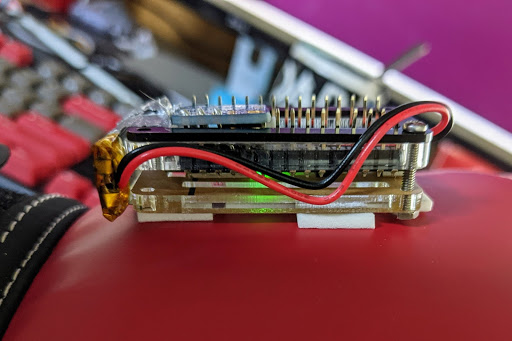
For wireless power, we used the Adafruit Li-Ion Battery Pack. If you do not have the battery pack, you can still walk through this tutorial using a suitably long micro USB cable to power the board. Though collecting gesture data is not quite as fun when you are wired. See the images below hooking up the battery to the Nano 33 BLE Sense.
Building Your Data Set
For every machine learning project, the quality of the final product depends on the quality of your data set. Time-series data, unlike image and audio, are typically unique to each application. Because of this, you often need to collect and annotate your datasets. The next part of this tutorial will walk you through how to connect to the Nano 33 BLE Sense to stream data wirelessly over BLE as well as label the data so it can be used to train a TensorFlow model.
For this project we are going to collect data for 5 different gestures as well as some data for negative cases which we will label as Unknown. The 5 boxing gestures we are going to collect data for are Jab, Overhand, Cross, Hook, and Uppercut.
We will also collect data on both the right and left glove. Giving us a total of 10 different classes. To simplify things we will build two separate models one for the right glove, and one for the left. This tutorial will focus on the left glove.
Streaming sensor data from the Nano 33 over BLE
The first challenge of a TinyML project is often to figure out how to get data off of the sensor. Depending on your needs you may choose Wi-Fi, BLE, Serial, or LoRaWAN. Alternatively, you may find storing data to an internal SD card and transferring the files after is the best way to collect data. For this tutorial, we will take advantage of the onboard BLE radio to stream sensor data from the Nano 33 BLE Sense.
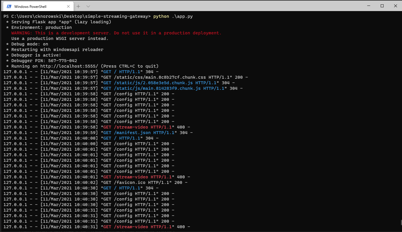
We are going to use the SensiML Open Gateway running on our computer to retrieve the sensor data. To download and launch the gateway open a terminal and run the following commands:
git clone https://github.com/sensiml/open-gateway

cd open-gateway
pip3 install -r requirements.txt
python3 app.py
The gateway should now be running on your machine.
Next, we need to connect the gateway server to the Nano 33 BLE Sense. Make sure you have flashed the Data Collection Firmware to your Nano 33. This firmware implements the Simple Streaming Interface specification which creates two topics used for streaming data. The /config topic returns a JSON describing the sensor data and /stream topic streams raw sensor data as a byte array of Int16 values.
To configure the gateway to connect to your sensor:
Go to the gateway address in your browser (defaults to localhost:5555)
Click on the Home Tab
Set Device Mode: Data Capture
Set Connection Type: BLE
Click the Scan button, and selectthe device named Nano 33 DCL
Click the Connect to Device button
The gateway will pull the configuration from your device, and be ready to start forwarding sensor data. You can verify it is working by going to the Test Stream tab and clicking the Start Stream button.
Setting up the Data Capture Lab Project
Now that we can stream data, the next step is to record and label the boxing gestures. To do that we will use the SensiML Data Capture Lab. If you haven’t already done so, download and install the Data Capture Lab to record sensor data.
We have created a template project to get you started. The project is prepopulated with the gesture labels and metadata information, along with some pre-recorded example gestures files. To add this project to your account:
Click Browse which will open the file explorer window
Navigate to the Boxing Glove Gestures Demo folder you just unzipped and select the Boxing Glove Gestures Demo.dclproj file
Click Upload
Connecting to the Gateway
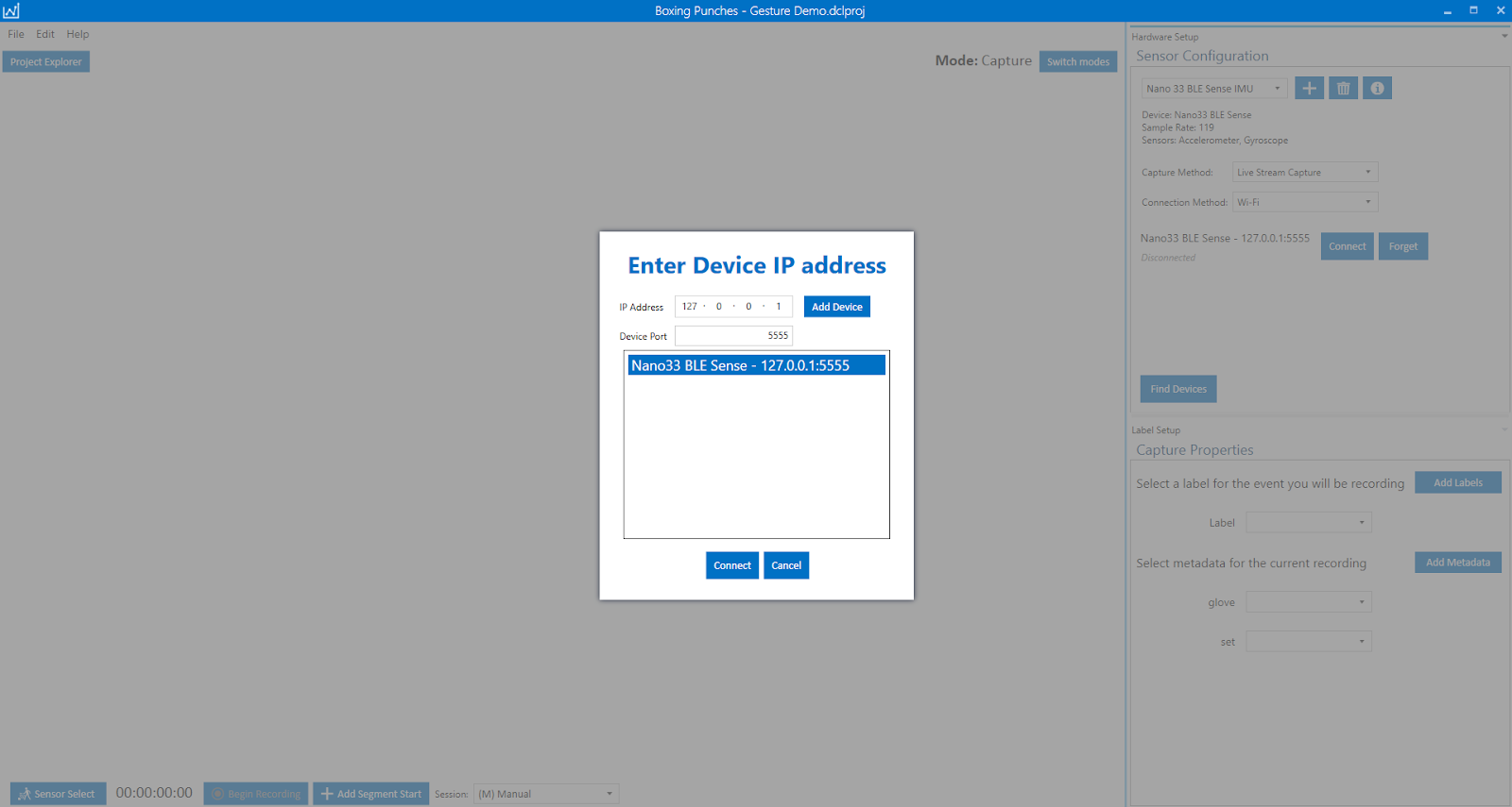
After uploading the project, you can start capturing sensor data. For this tutorial we will be streaming data to the Data Capture Lab from the gateway over TCP/IP. To connect to the Nano 33 BLE Sense from the Data Capture Lab through the gateway:
Open the Project Boxing Glove Gestures Demo
Click Switch Modes -> Capture Mode
Select Connection Method: Wi-Fi
Click the Find Devices button
Enter the IP Address of your gateway machine, and the port the server is running on (typically 127.0.0.1:5555)
Click Add Device
Select the newly added device
Click the Connect button
You should see sensor data streaming across the screen. If you are having trouble with this step, see the full documentation here for troubleshooting.
Capturing Boxing Gesture Sensor Data
The Data Capture Lab can also play videos that have been recorded alongside your sensor data. If you want to capture videos and sync them up with sensor data see the documentation here. This can be extremely helpful during the annotation phase to help interpret what is happening at a given point in the time-series sensor waveforms.
Now that data is streaming into the Data Capture Lab, we can begin capturing our gesture data set.
Select “Jab” from the Label dropdown in the Capture Properties screen. (this will be the name of the file)
Select the Metadata which captures the context (subject, glove, experience, etc.)
Then click the Begin Recording buttonto start recording the sensor data
Perform several “Jab” gestures
Click the Stop Recording button when you are finished
After you hit stop recording, the captured data will be saved locally and synced with the cloud project. You can view the file by going to the Project Explorer and double-clicking on the newly created file.
The following video walks through capturing sensor data.
Annotating Sensor Data
To classify sensor data in real-time, you need to decide how much and which portion of the sensor stream to feed to the classifier. On edge devices, it gets even more difficult as you are limited to a small buffer of data due to the limited RAM. Identifying the right segmentation algorithm for an application can save on battery life by limiting the number of classifications performed as well as improving the accuracy by identifying the start and end of a gesture.
Segmentation algorithms work by taking the input from the sensor and buffering the data until they determine a new segment has been found. At that point, they pass the data buffer down to the result of the pipeline. The simplest segmentation algorithm is a sliding window, which continually feeds a set chunk of data to the classifier. However, there are many drawbacks to the sliding window for discrete gesture recognition, such as performing classifications when there are no events. This wastes battery and runs the risk of having events split across multiple windows which can lower accuracy.
Segmenting in the Data Capture Lab
We identify events in the Data Capture Lab by creating Segments around the events in your sensor data. Segments are displayed with a pair of blue and red lines when you open a file and define where an event is located.
The Data Capture Lab has two methods for labeling your events: Manual and Auto. In manual mode you can manually drag and drop a segment onto the graph to identify an event in your sensor data. Auto mode uses a segmentation algorithm to automatically detect events based on customizable parameters. For this tutorial, we are going to use a segmentation algorithm in Auto mode. The segmentation algorithms we use for determining events will also be compiled as part of the firmware so that the on-device model will be fed the same segments of data it was trained against.
We have already created a segmentation algorithm for this project based on the dataset we have collected so far. To perform automatic event detection on newly captured data file:
Select the file from the Project Explorer
Click on the Detect Segments button
The segmentation algorithm will be run against the capture and the segments it finds will be added to the file
Note: If the events are not matching the real segments in your file, you may need to adjust the parameters of the segmentation algorithm.
Labeling Events in the Data Capture Lab
Keep in mind that automatic event detection only detects that an event has occurred, it does not determine what type of event has occurred. For each event that was detected, you will need to apply a label to them. To do that:
Select one or more of the segments from the graph
Click the Edit button or (Ctrl+E)
Specify which label is associated with that event
Repeat steps 1-3 for all segments in the capture
Click Save
Building a TinyML Model
We are going to use Google Colab to train our machine learning model using the data we collected from the Nano 33 BLE Sense in the previous section. Colab provides a Jupyter notebook that allows us to run our TensorFlow training in a web browser. Open the Google Colab notebook and follow along to train your model.
Offline Model Validation
After saving the model, go to the Analytic Studio to perform offline validation. To test the model against any of the captured data files
Open the Boxing Glove Gestures Demo project in the Summary Tab
Go to Test Model Tab
Select your model from the Model Name dropdown
Select one or more of the capture files by clicking on them
Click the Compute Accuracy Buttonto classify the captures using the selected model
p>When you click the Compute Accuracy button, the segmentation algorithm, preprocessing steps, and TensorFlow model are compiled into a single Knowledge Pack. Then the classification results and accuracy for each of the captures you selected are computed using the compiled Knowledge Pack. Click the Results button for the individual capture to see the classifications for all of the detected events and how they compared with the ground truth labels.
Deploy and Test on the Nano 33 BLE Sense
Downloading the model as firmware
Now that you validated the model offline, it’s time to see how it performs at the edge. To do that we download and flash the model to the Nano 33 BLE Sense.
Go to the Download Model tab of the Analytics Studio
Select the HW Platform:Arduino CortexM4
Select Format: Library
Click the Download button
The compiled library file should download to your computer
Flashing the Firmware
After downloading the library, we will build and upload the firmware to the Nano 33 BLE Sense. For this step, you will need the Nano 33 Knowledge Pack Firmware. To compile the firmware, we are using Visual Studio Code with the Platform IO plugin. To compile your model and Flash the Nano 33 BLE Sense with this firmware:
In the folder, you will find the following directories:
knowledgepack_project/
libsensiml/
Copy the files from libsensiml to nano33_knowledge_pack/lib/sensiml. You will overwrite the files included in the repository.
Copy the files from knowledgepack_project to nano33_knowledge_pack/src/
Switch to the Platform I/O extension tab in VS Code
Connect your Nano 33 BLE Sense to your computer using the micro USB cable.
Click Upload and Monitor under the nano33ble_with_tensorflow in the PlatformI/O tab.
When the device restarts, it will boot up and your model will be running automatically. The video below walks through these steps.
Viewing Classification Results
To see the classification results in real-time connect to your device over BLE using the Android TestApp or the SensiML Open Gateway. The device will show up with the name Nano33 SensiML KP when you scan for devices. We have trained two models, one for the left glove and one for the right glove. You can see a demo of both models running at the same time in the following video.
Conclusion
We hope this blog has given you the tools you need to start building an end-to-end TinyML application using TensorFlow Lite For Microcontrollers and the SensiML Analytics Toolkit. For more tutorials and examples of TinyML applications checkout the application examples in our documentation. Follow us on LinkedIn or get in touch with us, we love hearing about all of the amazing TinyML applications the community is working on!


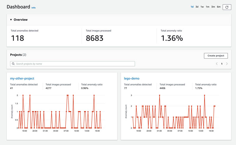
 Niklas Palm is a Solutions Architect at AWS in Stockholm, Sweden, where he helps customers across the Nordics succeed in the cloud. He’s particularly passionate about serverless technologies along with IoT and machine learning. Outside of work, Niklas is an avid cross-country skier and snowboarder as well as a master egg boiler.
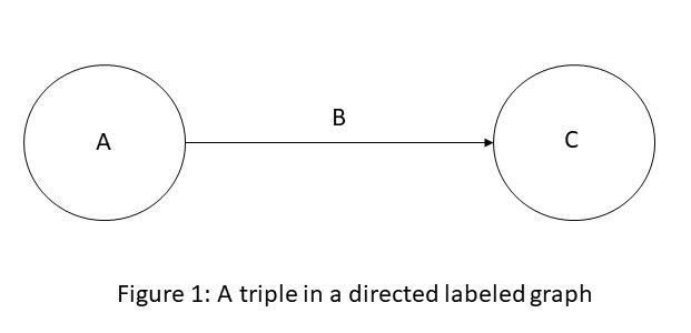
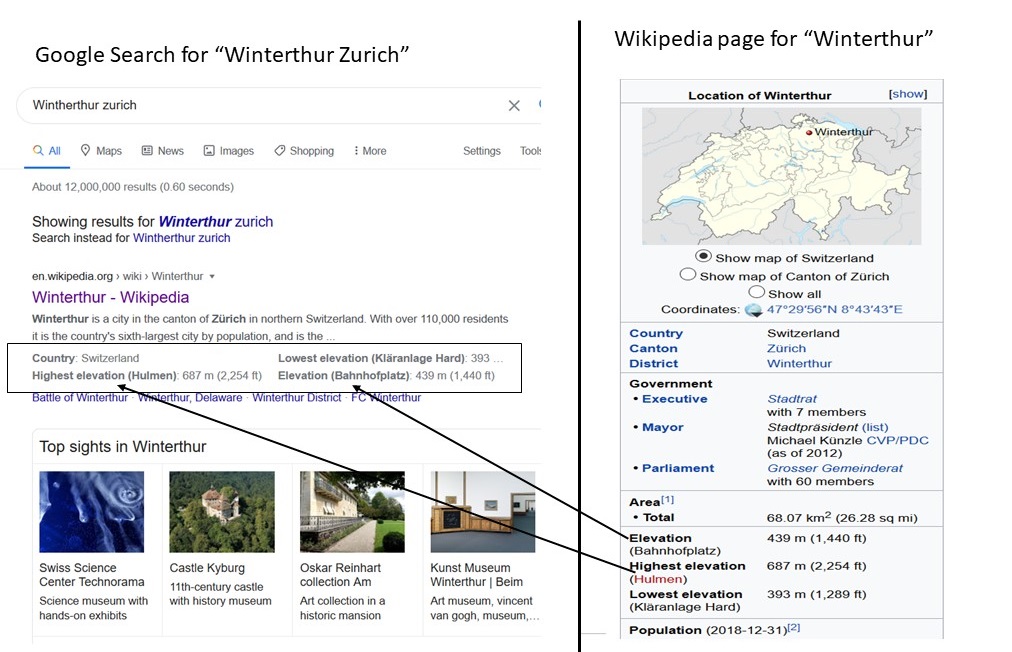
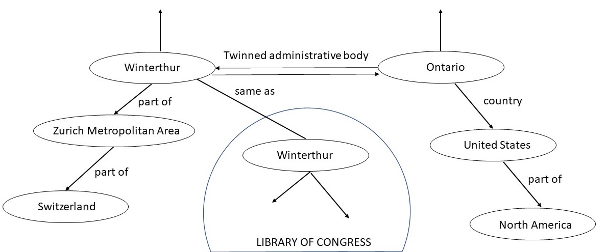
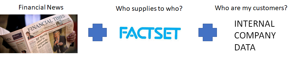
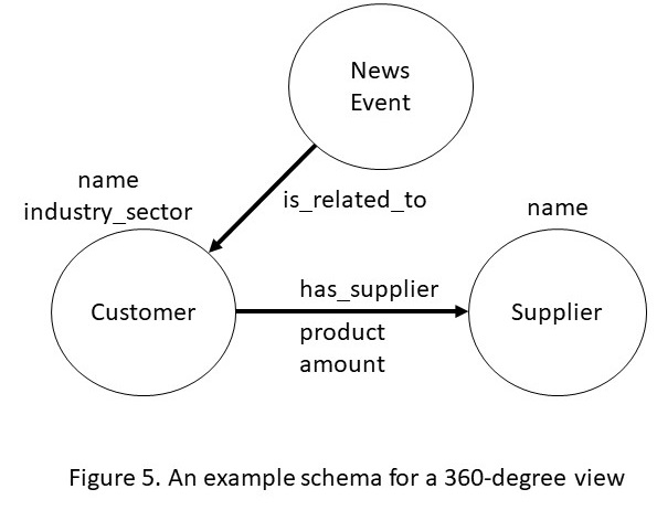
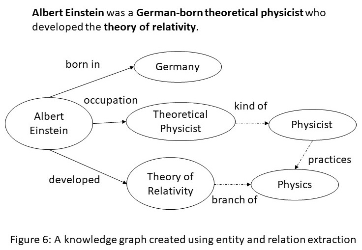
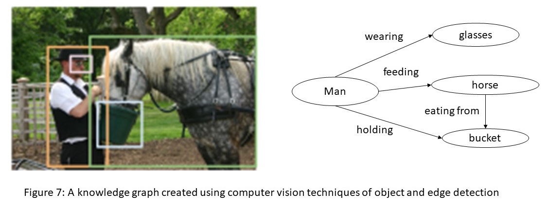


 Abhinav Jawadekar is a Senior Partner Solutions Architect at Amazon Web Services. Abhinav works with AWS partners to help them in their cloud journey.
 Udi Hershkovich has been a Principal WW AI/ML Service Specialist at AWS since 2018. Prior to AWS, Udi held multiple leadership positions with AI startups and Enterprise initiatives including co-founder and CEO at LeanFM Technologies, offering ML-powered predictive maintenance in facilities management, CEO of Safaba Translation Solutions, a machine translation startup acquired by Amazon in 2015, and Head of Professional Services for Contact Center Intelligence at Amdocs. Udi holds Law and Business degrees from the Interdisciplinary Center in Herzliya, Israel, and lives in Pittsburgh, Pennsylvania, USA.