How acoustic event detection helps Alexa Guard understand what might warrant an alert — and what just might be a microwave beeping.Read More
Prepare data for predicting credit risk using Amazon SageMaker Data Wrangler and Amazon SageMaker Clarify
For data scientists and machine learning (ML) developers, data preparation is one of the most challenging and time-consuming tasks of building ML solutions. In an often iterative and highly manual process, data must be sourced, analyzed, cleaned, and enriched before it can be used to train an ML model.
Typical tasks associated with data preparation include:
- Locating data – Finding where raw data is stored and getting access to it
- Data visualization – Examining statistical properties for each column in the dataset, building histograms, studying outliers
- Data cleaning – Removing duplicates, dropping or filling entries with missing values, removing outliers
- Data enrichment and feature engineering – Processing columns to build more expressive features, selecting a subset of features for training
Data scientists and developers typically iterate through these tasks until a model reaches the desired level of accuracy. This iterative process can be tedious, error-prone, and difficult to replicate as a deployable data pipeline. Fortunately, with Amazon SageMaker Data Wrangler, you can reduce the time it takes to prepare data for ML from weeks to minutes by accelerating the process of data preparation and feature engineering. With Data Wrangler, you can complete each step of the ML data preparation workflow, including data selection, cleansing, exploration, and visualization, with little to no code, which simplifies the data preparation process.
In a previous post introducing Data Wrangler, we highlighted its main features and walked through a basic example using the well-known Titanic dataset. For this post, we dive deeper into Data Wrangler and its integration with other Amazon SageMaker features to help you get started quickly.
Now, let’s get started with Data Wrangler.
Solution overview
In this post, we use Data Wrangler to prepare data for creating ML models to predict credit risk and help financial institutions more easily approve loans. The result is an exportable data flow capturing the data preparation steps required to prepare the data for modeling. We use a sample dataset containing information on 1,000 potential loan applications, built from the German Credit Risk dataset. This dataset contains categorical and numeric features covering the demographic, employment, and financial attributes of loan applicants, as well as a label indicating whether the individual is high or low credit risk. The features require cleaning and manipulation before we can use them as training data for an ML model. A modified version of the dataset, which we use in this post, has been saved in a sample data Amazon Simple Storage Service (Amazon S3) bucket. In the next section, we walk through how to download the sample data and upload it to your own S3 bucket.
The main ML workflow components that we focus on are data preparation, analysis, and feature engineering. We also discuss Data Wrangler’s integration with other SageMaker features as well as how to export the data flow for ease of use as a deployable data pipeline or submission to Amazon SageMaker Feature Store.
Data preparation and initial analysis
In this section, we download the sample data and save it in our own S3 bucket, import the sample data from the S3 bucket, and explore the data using Data Wrangler analysis features and custom transforms.
To get started with Data Wrangler, you need to first onboard to Amazon SageMaker Studio and create a Studio domain for your AWS account within a given Region. For instructions on getting started with Studio, see Onboard to Amazon SageMaker Studio or watch the video Onboard Quickly to Amazon SageMaker Studio. To follow along with this post, you need to download and save the sample dataset in the default S3 bucket associated with your SageMaker session, or in another S3 bucket of your choice. Run the following code in a SageMaker notebook to download the sample dataset and then upload it to your own S3 bucket:
from sagemaker.s3 import S3Uploader
import sagemaker
sagemaker_session = sagemaker.Session()
7#specify target location (modify to specify a location of your choosing)
bucket = sagemaker_session.default_bucket()
prefix = 'data-wrangler-demo'

#download data from sample data Amazon S3 bucket
!wget https://sagemaker-sample-files.s3.amazonaws.com/datasets/tabular/uci_statlog_german_credit_data/german_credit_data.csv

#upload data to your own Amazon S3 bucket
dataset_uri = S3Uploader.upload('german_credit_data.csv', 's3://{}/{}'.format(bucket,prefix))
print('Demo data uploaded to: {}'.format(dataset_uri))
Data Wrangler simplifies the data import process by offering connections to Amazon S3, Amazon Athena, and Amazon Redshift, which makes loading multiple datasets as easy as a couple of clicks. You can easily load tabular data into Amazon S3 and directly import it, or you can import the data using Athena. Alternatively, you can seamlessly connect to your Amazon Redshift data warehouse and quickly load your data. The ability to upload multiple datasets from different sources enables you to connect disparate data across sources.
With any ML solution, you iterate through exploratory data analysis (EDA) and data transformation until you have a suitable dataset for training a model. With Data Wrangler, switching between these tasks is as easy as adding a transform or analysis step into the data flow using the visual interface.
To start off, we import our German credit dataset, german_credit_data.csv, from Amazon S3 with a few clicks.
- On the Studio console, on the File menu, under New, choose Flow.

After we create this new flow, the first window we see has options related to the location of the data source that you want to import. You can import data from Amazon S3, Athena, or Amazon Redshift.
- Select Amazon S3 and navigate to the
german_credit_data.csvdataset that we stored in an S3 bucket.
You can review the details of the dataset, including a preview of the data in the Preview pane.
- Choose Import dataset.
We’re now ready to start exploring and transforming the data in our new Data Wrangler flow.

After the dataset is loaded, we can start by creating an analysis step to look at some summary statistics.
- From the data flow view, choose the plus sign (+ icon) and choose Add analysis.

This opens a new analysis view in which we can explore the DataFrame using visualizations such as histograms or scatterplots. You can also quickly view summary statistics.
- For Analysis type¸ choose Table Summary.
- Choose Preview.
Data Wrangler displays a table of statistics similar to the Pandas Dataframe.describe() method.

It may also be useful to understand the presence of null values in the data and view column data types.
- Navigate back to the data flow view by choosing the Prepare.
- In the data flow, choose Add Transform.
In this transform view, data transformation options are listed in the pane on the right, including an option to add a custom transform step.
- On the Custom Transform drop-down menu, choose Python (Pandas).
- Enter
df.info()into the code editor. - Choose Preview to run the snippet of Python code.
We can inspect the DataFrame information in the right pane while also looking at the dataset in the left pane.

- Return to the data flow view and choose Add analysis to analyze the data attributes.
Let’s look at the distribution of the target variable: credit risk.
- On the Analysis type menu, choose Histogram.
- For X axis, choose risk.
This creates a histogram that shows the risk distribution of applicants. We see that approximately 2/3 of applicants are labeled as low risk and approximately 1/3 of applicants are labeled as high risk.

Next, let’s look at the distribution of the age of credit applicants, colored by risk. We see that in younger age groups, a higher proportion of applicants have high risk.

We can continue to explore the distributions of other features such as risk by sex, housing type, job, or amount in savings account. We can use the Facet by option to explore the relationships between additional variables. In the next section, we move to the data transformation stage.
Data transformation and feature engineering
In this section, we complete the following:
- Separate concatenated string columns
- Recode string categorical variables to numeric ordinal and nominal categorical variables
- Scale numeric continuous variables
- Drop obsolete features
- Reorder columns
Data Wrangler contains numerous built-in data transformations so you can quickly clean, normalize, transform, and combine features. You can use these built-in data transformations without writing any code, or you can write custom transforms to make additional changes to the dataset such as encoding string categorical variables to specific numerical values.
- In the data flow view, choose the plus sign and choose Add transform.
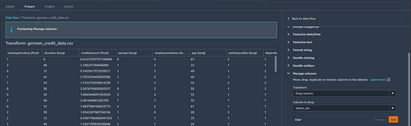
A new view appears that shows the first few lines of the dataset, as well as a list of over 300 built-in transforms. Let’s start with modifying the status_sex column. This column contains two values: sex and marital status. We first split the string into a list of two values separated by the delimiter : .
- Choose Search and Edit.
- On the Transform menu, choose Split string by delimiter.
- For Input column, choose the
status_sex. - For Delimiter, enter
:. - For Output column, enter a name (for this post, we use
vec).
We can further flatten this column in a later step.
- Choose Preview to review the changes.
- Choose Add.

- To flatten the column
vecwe just created, we can apply a Manage vectors transformation and choose Flatten.
The outputs are two columns: sex_split_0, the Sex column, and sex_split_1, the Marital Status column.

- To easily identify the features, we can rename these two columns to
sexandmarital_statususing the Manage columns transformation by choosing Rename column.

The current credit risk classification is indicated by string values. Low risk means that the user has good credit, and high risk means that the user has bad credit. We need to encode this target or label variable as a numeric categorical variable where 0 indicates low risk and 1 indicates high risk.
- To do that, we choose Encode categorical and choose the transform Ordinal encode.
- Output this revised feature to the output column target.
The classification column now indicates 0 for low risk and 1 for high risk.

Next, let’s encode the other categorical string variables.
- Starting with
existingchecking, we can again use Ordinal encode if we consider the categories no account, none, little, and moderate to have an inherent order.

- For greater control over the encoding of ordinal variables, you can choose Custom Transform and use Python (Pandas) to create a new custom transform for the dataset.
Starting with savings, we represent the amount of money available in a savings account with the following map: {'unknown': 0 ,little': 1, 'moderate': 2, 'high': 3, 'very high': 4}.
When you create custom transforms using Python (Pandas), the DataFrame is referenced as df.
- Enter the following code into the code editor cell:
# 'Savings' custom transform pandas code
savings_map = {'unknown': 0, 'little': 1,'moderate': 2,'high': 3,'very high': 4}
df['savings'] = df['savings'].map(savings_map).fillna(df['savings'])
- We do the same for
employmentsince:
# 'Employmentsince' custom transform pandas code
employment_map = { 'unemployed': 0,'1 year': 1,'1 to 4 years': 2,'4 to 7 years': 3,'7+ years': 4}
df['employmentsince'] = df['employmentsince'].map(employment_map).fillna(df['employmentsince'])

For more information about encoding categorical variables, see Custom Formula.
Other categorical variables that don’t have an inherent order also need to be transformed. We can use the Encode Categorical transform to one-hot encode these nominal variables. We one-hot encode housing, job, sex, and marital_status.
- Let’s start by encoding
housingby choosing One-hot encode on the Transform drop-down menu. - For Output style¸ choose Columns.

- Repeat for the remaining three nominal variables:
job,sex, andmarital_status.
After we encode all the categorical variables, we can address the numerical values. In particular, we can scale the numerical values in order to improve the performance of our future ML model.
- We do this by again choosing Add Transform and then Process numeric.
- From here you have the option of selecting between standard, robust, min-max, or max absolute scalars.

Before exporting the data, I remove the original string categorical columns that I encoded to numeric columns, so that our feature dataset contains only numbers, and therefore is machine-readable for training ML models.
- Choose Manage columns and choose the transform Drop column.
- Drop all the original categorical columns that contain string values such as
status_sex,risk, and the temporary columnvec.
As a final step, some ML libraries, such as XGBoost, expect the first column in the dataset to be the label or target variable.
- Use the Manage columns transform to move the target variable to the first column in the dataset.

We used custom and built-in transforms to create a training dataset that is ready for training an ML model. One tip for building out a data flow is to take advantage of the Previous steps tab in the right pane to walk through each step and view how the table changes after each transform. To change a step that is upstream, you have to delete all the downstream steps as well.
Further analysis and integration
In this section, we discuss opportunities for further data analysis and integration with SageMaker features.
Detect bias with Amazon SageMaker Clarify
Let’s explore Data Wrangler’s integration with other SageMaker features. In addition to the data analysis options available within Data Wrangler, you can also use Amazon SageMaker Clarify to detect potential bias during data preparation, after model training, and in your deployed model. In many use cases for detecting and analyzing bias in data and models, Clarify can be a great asset, including this credit application use case.
In this use case, we use Clarify to check for class imbalance and bias against one feature: sex. Clarify is integrated into Data Wrangler as part of the analysis capabilities, so we can easily create a bias report by adding a new analysis, choosing our target column, and selecting the column we want to analyze for bias. In this case, we use the sex column as an example, but you could continue to explore and analyze bias for other columns.

The bias report is generated by Clarify that operates within Data Wrangler. This report provides the following default metrics: class imbalance, difference in positive proportions in labels, and Jensen-Shannon Divergences. A short description provides instructions on how to read each metric. In our example, the report indicates that the data may be imbalanced. We should consider using sampling methods to correct this imbalance in our training data. For more information about Clarify capabilities and how to create a Clarify processing job using the SageMaker Python SDK, see New – Amazon SageMaker Clarify Detects Bias and Increases the Transparency of Machine Learning Models.
Support rapid model prototyping with Data Wrangler Quick Model visualization
Let’s now use Data Wrangler’s Quick Model analysis, which allows you to quickly evaluate your data and produce importance scores for each potential feature that you may consider including in an ML model, now that your data preparation data flow is complete. The Quick Model analysis gives you a feature importance score for each variable in the data, indicating how useful a feature is at predicting the target label.
This Quick Model also provides an overall model score. For a classification problem, such as our use case of predicting high or low credit risk, the Quick Model also provides an F1 score. This gives an indication of potential model fit using the data as you’ve prepared it in your complete data flow. For regression problems, the model provides a mean squared error (MSE) score. In the following screenshot, we can see which features contribute most to the predicted outcome: existing checking, credit amount, duration of loan, and age. We can use this information to inform our model development approach or make additional adjustments to our data flow, such as dropping additional columns with low feature importance.

Use Data Wrangler data flows in ML deployments
After you complete your data transformation steps and analysis, you can conveniently export your data preparation workflow flow. When you export your data flow, you have the option of exporting to the following:
- A notebook running the data flow as a Data Wrangler job – Exporting as a Data Wrangler job and running the resulting notebook takes the data processing steps defined in your .flow file and generates a SageMaker processing job to run these steps on your entire source dataset, providing a way to save processed data as a CSV or Parquet file to Amazon S3.
- A notebook running the data flow as an Amazon SageMaker Pipelines workflow – With Amazon SageMaker Pipelines, you can create end-to-end workflows that manage and deploy SageMaker jobs responsible for data preparation, model training, and model deployment. By exporting your Data Wrangler flow to Pipelines, a Jupyter notebook is created that, when run, defines a data transformation pipeline following the data processing steps defined in your .flow file.
- Python code replicating the steps in the Data Wrangler data flow – Exporting as a Python file enables you to manually integrate the data processing steps defined in your flow into any data processing workflow.
- A notebook pushing your processed features to Feature Store – When you export to Feature Store and run the resulting notebook, your data can be processed as a SageMaker processing job, and then ingested into an online and offline feature store.

Conclusion
In this post, we explored the German credit risk dataset to understand the transformation steps needed to prepare the data for ML modeling so financial institutions can approve loans more easily. We then created ordinal and one-hot encoded features from the categorical variables, and finally scaled our numerical features—all using Data Wrangler. We now have a complete data transformation data flow that has transformed our raw dataset into a set of features ready for training an ML model to predict credit risk among credit applicants.
The options to export our Data Wrangler data flow allow us to use the transformation pipeline as a Data Wrangler processing job, create a feature store to better store and track features to be used in future modeling, or save the transformation steps as part of a complete SageMaker pipeline in your ML workflow. Data Wrangler makes it easy to work interactively on data preparation steps before transforming them into code that can be used immediately for ML model experimentation and into production.
To learn more about Amazon SageMaker Data Wrangler, visit the webpage. Give Data Wrangler a try, and let us know what you think in the comments!
About the Author
Courtney McKay is a Senior Principal with Slalom Consulting. She is passionate about helping customers drive measurable ROI with AI/ML tools and technologies. In her free time, she enjoys camping, hiking and gardening.
Learning to Manipulate Deformable Objects
Posted by Daniel Seita, Research Intern and Andy Zeng, Research Scientist, Robotics at Google
While the robotics research community has driven recent advances that enable robots to grasp a wide range of rigid objects, less research has been devoted to developing algorithms that can handle deformable objects. One of the challenges in deformable object manipulation is that it is difficult to specify such an object’s configuration. For example, with a rigid cube, knowing the configuration of a fixed point relative to its center is sufficient to describe its arrangement in 3D space, but a single point on a piece of fabric can remain fixed while other parts shift. This makes it difficult for perception algorithms to describe the complete “state” of the fabric, especially under occlusions. In addition, even if one has a sufficiently descriptive state representation of a deformable object, its dynamics are complex. This makes it difficult to predict the future state of the deformable object after some action is applied to it, which is often needed for multi-step planning algorithms.
In “Learning to Rearrange Deformable Cables, Fabrics, and Bags with Goal-Conditioned Transporter Networks,” to appear at ICRA 2021, we release an open-source simulated benchmark, called DeformableRavens, with the goal of accelerating research into deformable object manipulation. DeformableRavens features 12 tasks that involve manipulating cables, fabrics, and bags and includes a set of model architectures for manipulating deformable objects towards desired goal configurations, specified with images. These architectures enable a robot to rearrange cables to match a target shape, to smooth a fabric to a target zone, and to insert an item in a bag. To our knowledge, this is the first simulator that includes a task in which a robot must use a bag to contain other items, which presents key challenges in enabling a robot to learn more complex relative spatial relations.
The DeformableRavens Benchmark
DeformableRavens expands our prior work on rearranging objects and includes a suite of 12 simulated tasks involving 1D, 2D, and 3D deformable structures. Each task contains a simulated UR5 arm with a mock gripper for pinch grasping, and is bundled with scripted demonstrators to autonomously collect data for imitation learning. Tasks randomize the starting state of the items within a distribution to test generality to different object configurations.
 |
| Examples of scripted demonstrators for manipulation of 1D (cable), 2D (fabric), and 3D (bag) deformable structures in our simulator, using PyBullet. These show three of the 12 tasks in DeformableRavens. Left: the task is to move the cable so it matches the underlying green target zone. Middle: the task is to wrap the cube with the fabric. Right: the task is to insert the item in the bag, then to lift and move the bag to the square target zone. |
Specifying goal configurations for manipulation tasks can be particularly challenging with deformable objects. Given their complex dynamics and high-dimensional configuration spaces, goals cannot be as easily specified as a set of rigid object poses, and may involve complex relative spatial relations, such as “place the item inside the bag”. Hence, in addition to tasks defined by the distribution of scripted demonstrations, our benchmark also contains goal-conditioned tasks that are specified with goal images. For goal-conditioned tasks, a given starting configuration of objects must be paired with a separate image that shows the desired configuration of those same objects. A success for that particular case is then based on whether the robot is able to get the current configuration to be sufficiently close to the configuration conveyed in the goal image.
Goal-Conditioned Transporter Networks
To complement the goal-conditioned tasks in our simulated benchmark, we integrated goal-conditioning into our previously released Transporter Network architecture — an action-centric model architecture that works well on rigid object manipulation by rearranging deep features to infer spatial displacements from visual input. The architecture takes as input both an image of the current environment and a goal image with a desired final configuration of objects, computes deep visual features for both images, then combines the features using element-wise multiplication to condition pick and place correlations to manipulate both the rigid and deformable objects in the scene. A strength of the Transporter Network architecture is that it preserves the spatial structure of the visual images, which provides inductive biases that reformulate image-based goal conditioning into a simpler feature matching problem and improves the learning efficiency with convolutional networks.
An example task involving goal-conditioning is shown below. In order to place the green block into the yellow bag, the robot needs to learn spatial features that enable it to perform a multi-step sequence of actions to spread open the top opening of the yellow bag, before placing the block into it. After it places the block into the yellow bag, the demonstration ends in a success. If in the goal image the block were placed in the blue bag, then the demonstrator would need to put the block in the blue bag.
 |
| An example of a goal-conditioned task in DeformableRavens. Left: A frontal camera view of the UR5 robot and the bags, plus one item, in a desired goal configuration. Middle: The top-down orthographic image of this setup, which is size 160×320 and passed as the goal image to specify the task success criterion. Right: A video of the demonstration policy showing that the item goes into the yellow bag, instead of the blue one. |
Results
Our results suggest that goal-conditioned Transporter Networks enable agents to manipulate deformable structures into flexibly specified configurations without test-time visual anchors for target locations. We also significantly extend prior results using Transporter Networks for manipulating deformable objects by testing on tasks with 2D and 3D deformables. Results additionally suggest that the proposed approach is more sample-efficient than alternative approaches that rely on using ground-truth pose and vertex position instead of images as input.
For example, the learned policies can effectively simulate bagging tasks, and one can also provide a goal image so that the robot must infer into which bag the item should be placed.
 |
| An example of policies trained using Transporter Networks applied in action on bagging tasks, where the objective is to first open the bag, then to put one (left) or two (right) items in the bag, then to insert the bag into the target zone. The left animation is zoomed in for clarity. |
 |
| An example of the learned policy using Goal-Conditioned Transporter Networks. Left: The frontal camera view. Middle: The goal image that the Goal-Conditioned Transporter Network receives as input, which shows that the item should go in the red bag, instead of the blue distractor bag. Right: The learned policy putting the item in the red bag, instead of the distractor bag (colored yellow in this case). |
We encourage other researchers to check out our open-source code to try the simulated environments and to build upon this work. For more details, please check out our paper.
Future Work
This work exposes several directions for future development, including the mitigation of observed failure modes. As shown below, one failure is when the robot pulls the bag upwards and causes the item to fall out. Another is when the robot places the item on the irregular exterior surface of the bag, which causes the item to fall off. Future algorithmic improvements might allow actions that operate at a higher frequency rate, so that the robot can react in real time to counteract such failures.
 |
| Examples of failure cases from the learned Transporter-based policies on bag manipulation tasks. Left: the robot inserts the cube into the opening of the bag, but the bag pulling action fails to enclose the cube. Right: the robot fails to insert the cube into the opening, and is unable to perform recovery actions to insert the cube in a better location. |
Another area for advancement is to train Transporter Network-based models for deformable object manipulation using techniques that do not require expert demonstrations, such as example-based control or model-based reinforcement learning. Finally, the ongoing pandemic limited access to physical robots, so in future work we will explore the necessary ingredients to get a system working with physical bags, and to extend the system to work with different types of bags.
Acknowledgments
This research was conducted during Daniel Seita’s internship at Google’s NYC office in Summer 2020. We thank our collaborators Pete Florence, Jonathan Tompson, Erwin Coumans, Vikas Sindhwani, and Ken Goldberg.

AI Slam Dunk: Startup’s Checkout-Free Stores Provide Stadiums Fast Refreshments
With live sports making a comeback, one thing remains a constant: Nobody likes to miss big plays while waiting in line for a cold drink or snack.
Zippin offers sports fans checkout-free refreshments, and it’s racking up wins among stadiums as well as retailers, hotels, apartments and offices. The startup, based in San Francisco, develops image-recognition models that run on the NVIDIA Jetson edge AI platform to help track customer purchases.
People can simply enter their credit card details into the company’s app, scan into a Zippin-driven store, grab a cold one and any snacks, and go. Their receipt is available in the app afterwards. Customers can also bypass the app and simply use a credit card to enter the stores and Zippin automatically keeps track of their purchases and charges them.
“We don’t want fans to be stuck waiting in line,” said Motilal Agrawal, co-founder and chief scientist at Zippin.
As sports and entertainment venues begin to reopen in limited capacities, Zippin’s grab-and-go stores are offering quicker shopping and better social distancing without checkout lines.
Zippin is a member of NVIDIA Inception, a virtual accelerator program that helps startups in AI and data science get to market faster. “The Inception team met with us, loaned us our first NVIDIA GPU and gave us guidance on NVIDIA SDKs for our application,” he said.
Streak of Stadiums
Zippin has launched in three stadiums so far, all in the U.S. It’s in negotiations to develop checkout-free shopping for several other major sports venues in the country.
In March, the San Antonio Spurs’ AT&T Center reopened with limited capacity for the NBA season, unveiling a Zippin-enabled Drink MKT beverage store. Basketball fans can scan in with the Zippin mobile app or use their credit card, grab drinks and go. Cameras and shelves with scales identify purchases to automatically charge customers.
The debut in San Antonio comes after Zippin came to Mile High Stadium, in Denver, in November, for limited capacity Broncos games. Before that, Zippin unveiled its first stadium, the Golden 1 Center, in Sacramento. It allows customers to purchase popcorn, draft beer and other snacks and drinks and is open for Sacramento Kings basketball games and concerts.
“Our mission is to accelerate the adoption of checkout-free stores, and sporting venues are the ideal location to benefit from our approach,” Agrawal said.
Zippin Store Advances
In addition to stadiums, Zippin has launched stores within stores for grab-and-go food and beverages in Lojas Americanas, a large retail chain in Brazil.
In Russia, the startup has put a store within a store inside an Azbuka Vkusa supermarket chain store located in Moscow. Zippin is also in Japan, where it has a pilot store in Tokyo with Lawson, a convenience store chain in an office location and another store within the Yokohama Techno Tower Hotel.
As an added benefit for retailers, Zippin’s platform can track products to help automate inventory management.
“We provide a retailer dashboard to see how much inventory there is for each individual item and which items have run low on stock. We can help to know exactly how much is in the store — all these detailed analytics are part of our offering,” Agrawal said.
Jetson Processing
Zippin relies on the NVIDIA Jetson AI platform for inference at 30 frames per second for its models, enabling split-second decisions on customer purchases. The application’s processing speed means it can keep up with a crowded store.
The company runs convolutional neural networks for product identification and store location identification to help track customer purchases. Also, using Zippin’s retail implementations, stores utilize smart shelves to determine whether a product was removed or replaced on a shelf.
The NVIDIA edge AI-driven platform can then process the shelf data and the video data together — sensor fusion — to determine almost instantly who grabbed what.
“It can deploy and work effectively on two out of three sensors (visual, weight and location) and then figure out the products on the fly, with training ongoing in action in deployment to improve the system,” said Agrawal.
The post AI Slam Dunk: Startup’s Checkout-Free Stores Provide Stadiums Fast Refreshments appeared first on The Official NVIDIA Blog.
Amazon Alexa scientist Yang Liu named an ISCA Fellow
Principal scientist will be recognized at Interspeech 2021.Read More
Maximize TensorFlow performance on Amazon SageMaker endpoints for real-time inference
Machine learning (ML) is realized in inference. The business problem you want your ML model to solve is the inferences or predictions that you want your model to generate. Deployment is the stage in which a model, after being trained, is ready to accept inference requests. In this post, we describe the parameters that you can tune to maximize performance of both CPU-based and GPU-based Amazon SageMaker real-time endpoints. SageMaker is a managed, end-to-end service for ML. It provides data scientists and MLOps teams with the tools to enable ML at scale. It provides tools to facilitate each stage in the ML lifecycle, including deployment and inference.
SageMaker supports both real-time inference with SageMaker endpoints and offline and temporary inference with SageMaker batch transform. In this post, we focus on real-time inference for TensorFlow models.
Performance tuning and optimization
For model inference, we seek to optimize costs, latency, and throughput. In a typical application powered by ML models, we can measure latency at various time points. Throughput is usually bounded by latency. Costs are calculated based on instance usage, and price/performance is calculated based on throughput and SageMaker ML instance cost per hour. Finally, as we continue to advance rapidly in all aspects of ML including low-level implementations of mathematical operations in chip design, hardware-specific libraries will play a greater role in performance optimization. Rapid experimentation that SageMaker facilitates is the lynchpin in achieving business objectives in a cost-effective, timely, and performant manner.
Performance tuning and optimization is an empirical field. The number of parameters to tune is combinatorial such that each set of configuration parameter values aren’t independent of each other. Various factors such as payload size, network hops, nature of hops, model graph features, operators in the model, and the model’s CPU, GPU, memory, and I/O profiles affect the optimal parameter tuning. The distribution of these effects on performance is a vast unexplored space. Therefore, we begin by describing these different parameters and recommend an empirical approach to tune these parameters and understand their effects on your model performance.
Based on our past observations, the function of effect of these parameters on an inference workload is, approximately, plateau-shaped or Gaussian-uniform. The values to maximize the performance of an endpoint lie along the ascendant curve of this distribution, demarcated by latencies. Typically, latencies increase with an increase in throughput. Improvements in throughput levels out or plateaus at a point where respective increases in concurrent connections don’t result in any significant improvement in throughput. Certain cases may show a detrimental effect from increasing certain parameters, such that the throughput rapidly decreases as the system is saturated with overhead.
The following chart illustrates transactions per second demarcated by latencies.

SageMaker TensorFlow Deep Learning Containers (DLCs) recently introduced new parameters to help with performance optimization of a CPU-based or GPU-based endpoint. As we discussed earlier, an ideal value of each of these parameters is subjective to factors such as model, model input size, batch size, endpoint instance type, and payload. What follows next is a description of these tunable parameters.
TensorFlow serving
We start with parameters related to TensorFlow serving.
SAGEMAKER_TFS_INSTANCE_COUNT
For TensorFlow-based models, the tensorflow_model_server binary is the operational piece that is responsible for loading a model in memory, running inputs against a model graph, and deriving outputs. Typically, a single instance of this binary is launched to serve models in an endpoint. This binary is internally multi-threaded and spawns multiple threads to respond to an inference request. In certain instances, if you observe that the CPU is respectably employed (over 30% utilized) but the memory is underutilized (less than 10% utilization), increasing this parameter might help. We have observed in our experiments that increasing the number of tensorflow_model_servers available to serve typically increases the throughput of an endpoint.
SAGEMAKER_TFS_FRACTIONAL_GPU_MEM_MARGIN
This parameter governs the fraction of the available GPU memory to initialize CUDA/cuDNN and other GPU libraries. 0.2 means 20% of the available GPU memory is reserved for initializing CUDA/cuDNN and other GPU libraries, and 80% of the available GPU memory is allocated equally across the TF processes. GPU memory is pre-allocated unless the allow_growth option is enabled.
Deep learning operators
Operators are nodes in a deep learning graph that perform mathematical operations on data. These nodes can be independent of each other and therefore can be run in parallel. In addition, you can internally parallelize nodes for operators such as tf.matmul() and tf.reduce_sum(). Next, we describe two parameters to control running these two operators using the TensorFlow threadpool.
SAGEMAKER_TFS_INTER_OP_PARALLELISM
This ties back to the inter_op_parallelism_threads variable. This variable determines the number of threads used by independent non-blocking operations. 0 means that the system picks an appropriate number.
SAGEMAKER_TFS_INTRA_OP_PARALLELISM
This ties back to the intra_op_parallelism_threads variable. This determines the number of threads that can be used for certain operations like matrix multiplication and reductions for speedups. A value of 0 means that the system picks an appropriate number.
Architecture for serving an inference request over HTTP
Before we look at the next set of parameters, let’s understand the typical arrangement when we deploy Nginx and Gunicorn to frontend tensorflow_model_server. Nginx is responsible for listening on port 8080; it accepts a connection and forwards it to Gunicorn, which serves as a Python HTTP Web Server Gateway Interface. Gunicorn is responsible for replying to /ping and forwarding /invocations to tensorflow_model_server. While replying to /invocations, Gunicorn invokes tensorflow_model_server with the payload.
The following diagram illustrates the anatomy of a SageMaker endpoint.

SAGEMAKER_GUNICORN_WORKERS
This governs the number of worker processes that Gunicorn is requested to spawn for handling requests. This value is used in combination with other parameters to derive a set that maximizes inference throughput. In addition to this, SAGEMAKER_GUNICORN_WORKER_CLASS governs the type of workers spawned, typically async, typically gevent.
OpenMP (Open Multi-Processing)
OpenMP is an implementation of multithreading, a method of parallelizing whereby a primary thread (a series of instructions ran consecutively) forks a specified number of sub-threads and the system divides a task among them. The threads then run concurrently, with the runtime environment allocating threads to different processors. Various parameters control the behavior of this library; in this post, we explore the impact of changing one of these many parameters. For a full list of parameters available and their intended use, refer to Environment Variables.
OMP_NUM_THREADS
Python internally uses OpenMP for implementing multithreading within processes. Typically, threads equivalent to the number of CPU cores are spawned. But when implemented on top of a Simultaneous Multi Threading (SMT) such Intel’s HypeThreading, a certain process might oversubscribe a particular core by spawning twice the threads as the number of actual CPU cores. In certain cases, a Python binary might end up spawning up to four times the threads as available actual processor cores. Therefore, an ideal setting for this parameter, if you have oversubscribed available cores using worker threads, is 1 or half the number of CPU cores on a SMT-enabled CPU.
In our experiments, we changed the values of these parameters as a tuple and not independently. Therefore, all the results and guidance assume the preceding scenario. As the results illustrate, we observed an increase of over 1,900% to over 87% in some models.
The following table shows an increase in TPS by adjusting parameters for a retrieval type model on an ml.c5.9xlarge instance.
| Number of workers | Number of TFS | OMP_NUM_THREAD | Inter Op Parallelization | Intra Op Parallelization | TPS |
| 1 | 1 | 36 | 36 | 36 | 15.87 |
| 36 | 1 | 1 | 36 | 36 | 164 |
| 1 | 1 | 1 | 1 | 1 | 33.0834 |
| 36 | 1 | 1 | 1 | 1 | 67.5118 |
| 36 | 8 | 1 | 1 | 1 | 319.078 |
The following table shows an increase in TPS by adjusting parameters for a Single Shot Detector type model on an ml.p3.2xlarge instance.
| Number of workers | Number of TFS | OMP_NUM_THREAD | Inter Op Parallelization | Intra Op Parallelization | TPS |
| 1 | 1 | 36 | 36 | 36 | 16.4613 |
| 1 | 1 | 1 | 36 | 36 | 17.1414 |
| 36 | 1 | 1 | 36 | 36 | 22.7277 |
| 1 | 1 | 1 | 1 | 1 | 16.7216 |
| 36 | 1 | 1 | 1 | 1 | 22.0933 |
| 1 | 4 | 1 | 1 | 1 | 16.6026 |
| 16 | 4 | 1 | 1 | 1 | 31.1001 |
| 36 | 4 | 1 | 1 | 1 | 30.9372 |
The following diagram shows the resultant increase in TPS by adjusting parameters.

Observe results in your own environments
Now that you know about these various parameters, how can you try them out in your environments? We first discuss how to set up these parameters, then describe a tool and methodology to test it and observe variations in latency and throughput.
Set up an endpoint with custom parameters
When you create a SageMaker endpoint, you can set values of these parameters by passing them in a dictionary for the env parameter in sagemaker.model.Model. See the following example code:
sagemaker_model = Model(image_uri=image_uri,
                        model_data=model_location_in_s3,
                        role=get_execution_role(),
                        env={'SAGEMAKER_GUNICORN_WORKERS': ’10’,
                             'SAGEMAKER_TFS_INSTANCE_COUNT': ’20’,
                             'OMP_NUM_THREADS': '1',
                             'SAGEMAKER_TFS_INTER_OP_PARALLELISM': '4',
                             'SAGEMAKER_TFS_INTRA_OP_PARALLELISM': '1'})
predictor = sagemaker_model.deploy(initial_instance_count=1,instance_type=test_instance_type, wait=True, endpoint_name=endpoint_name)
Test for success
Now that our parameters are set up, how do we test for success? How do we standardize a test that is uniform across our runs? We recommend the open-source tool Locust. In its simplest form, it allows us to control the number of concurrent connections being sent across to a target (in this case, SageMaker endpoints). Via one concurrent connection, we’re invoking inference (using invoke_endpoint) as fast as possible, sequentially. So, although the connections (users in Locust parlance) are concurrent, the invocations against the endpoint requesting inference are sequential.
The following graph shows invocations tracked with respect to Locust users peaking at about over 45,000 (with 95 TFS server spawned).

The following graph shows invocations for same instance peaking at around 11,000 (with 1 TFS server spawned).

This allows us to observe, as an output of this Locust command, the end-to-end P95 latency and TPS for the duration of test. So roughly speaking, lower latency and higher TPS (users) is better. As we tune our parameters, we observe TPS ascend delta between two users (n and n+1), and test for it to reach a point at which with every respective increase in users, the TPS stays constant. At such a point, past a certain number of users, the latency usually explodes due to resource contention in the endpoint. The point just before this latency explosion is where we have an endpoint at its functional best.
Although we observe this increase in TPS and decrease in latency while we tune parameters, you should also focus on two other metrics: average CPU utilization and average memory utilization. When you’re adjusting the number of SAGEMAKER_GUNICORN_WORKERS and SAGEMAKER_TFS_INSTANCE_COUNT, your aim should be to drive both CPU and memory to the maximum and treat that as a soft threshold to understand the high watermark for the throughput of this particular endpoint. The hard threshold is the latency that you can tolerate.
The following graph tracks an increase in ModelLatency with respect to increased load.

The following graph tracks an increase in CPUUtilization with respect to increased load.

The following graph tracks in increase in MemoryUtilization with respect to increased load.

Other optimizations to consider
You should consider a few other optimizations to further maximize the performance of your endpoint:
- To further enhance performance, optimize the model graph by compiling, pruning, fusing, and so on.
- You can also export models to an intermediate representation such as ONNX and use ONNX runtime for inference.
- Inputs can be batched, serialized, compressed, and passed over the wire in binary format to save bandwidth and maximize utilization.
- You can compile the TensorFlow Model Server binary to use hardware-specific optimizations (such as Intel optimizations like AVX-512 and MKL) or model optimizations such as compilation provided by SageMaker Neo. You can also use an optimized inference chip such as AWS Inferentia to further improve performance.
- In SageMaker, you can gain an additional performance boost by deploying models with automatic scaling.
Conclusion
In this post, we explored a few parameters that you can use to maximize the performance of a TensorFlow-based SageMaker real-time endpoint. These parameters are in essence overprovisioning serving processes and adjusting their parallel processing capabilities. As we saw in the tables, this overprovisioning and adjustment leads to better utilization of resources and higher throughput, sometimes an increase as much as 1,000%.
Although the best way to derive the correct values is through experimentation, by observing the combinations of different parameters and its effect on performance across ML models and SageMaker ML instances, you can start to build empirical knowledge on performance tuning and optimization.
SageMaker provides the tools to remove the undifferentiated heavy lifting from each stage of the ML lifecycle, thereby facilitating rapid experimentation and exploration needed to fully optimize your model deployments.
For more information, see Maximize TensorFlow* Performance on CPU: Considerations and Recommendations for Inference Workloads, Meaning of inter_op_parallelism_threads and intra_op_parallelism_threads, and the model SageMaker inference API.
About the Authors
 Chaitanya Hazarey is a Senior ML Architect with the Amazon SageMaker team. He focuses on helping customers design, deploy, and scale end-to-end ML pipelines in production on AWS. He is also passionate about improving explainability, interpretability, and accessibility of AI solutions.
 Karan Kothari is a software engineer at Amazon Web Services. He is on the Elastic Inference team working on building Model Server focused towards low latency inference workloads.
 Liang Ma is a software engineer at Amazon Web Services and is fascinated with enabling customers on their AI/ML journey in the cloud to become AWSome. He is also passionate about serverless architectures, data visualization, and data systems.
 Santosh Bhavani is a Senior Technical Product Manager with the Amazon SageMaker Elastic Inference team. He focuses on helping SageMaker customers accelerate model inference and deployment. In his spare time, he enjoys traveling, playing tennis, and drinking lots of Pu’er tea.
 Aaron Keller is a Senior Software Engineer at Amazon Web Services. He works on the real-time inference platform for Amazon SageMaker. In his spare time, he enjoys video games and amateur astrophotography.
Build BI dashboards for your Amazon SageMaker Ground Truth labels and worker metadata
This is the second in a two-part series on the Amazon SageMaker Ground Truth hierarchical labeling workflow and dashboards. In Part 1: Automate multi-modality, parallel data labeling workflows with Amazon SageMaker Ground Truth and AWS Step Functions, we looked at how to create multi-step labeling workflows for hierarchical label taxonomies using AWS Step Functions. In Part 2, we look at how to build dashboards and derive insights for analyzing dataset annotations and worker performance metrics on data lakes generated as output from the complex workflows.
Amazon SageMaker Ground Truth (Ground Truth) is a fully managed data labeling service that makes it easy to build highly accurate training datasets for machine learning (ML). This post introduces a solution that you can use to create customized business intelligence (BI) dashboards using Ground Truth labeling job output data. You can use these dashboards to analyze annotation quality, worker metrics, and more.
In Part 1, we presented a solution to create multiple types of annotations for a single input data object and check annotation quality, using a series of multi-step labeling jobs that run in a parallel, hierarchical fashion using Step Functions. The solution results in high-quality annotations using Ground Truth. The format of these annotations is explained in Output Data, and each takes the form of one or more JSON manifest files in Amazon Simple Storage Service (Amazon S3). You now need a mechanism to dynamically fetch these manifests, publish them on to your analytical datastore, and use them to create meaningful reports in an automated fashion. This allows ML practitioners and data scientists to track annotation progress and quality and allows MLOps and annotation operations teams to gain insights about the annotations and track worker performance. For example, these interested parties may want to see the following reports generated from Ground Truth output data:
- Annotation-level reports – These reports include the following:
- The number of annotations done in a specified time frame.
- Filtering based on label attributes. A label attribute is a Ground Truth feature that workers can use to provide metadata about individual annotations. For example, you can create a label attribute to have workers identify vehicle type (sedan, SUV, bus) or vehicle status (parked or moving).
- The number of frames per label or frame attributes in a labeling job. A frame attribute is a Ground Truth feature that workers can use to provide metadata about video frames. For example, you can create a frame attribute to have workers identify frame quality (blurry or clear) and add a visualization to show the number of good (clear) vs. bad (blurry) frames.
- The number of tasks audited or adjusted by a reviewer (in Part 1, this is a second-level or third-level worker).
- If you have workers audit labels from previous labeling jobs, you can enumerate audit results for each label (such as car or bush) using label attributes (such as correctly or incorrectly labeled).
- Worker-level reports – These reports include the following:
- The number of Ground Truth jobs worked on by each worker.
- The total number of labels created by each individual annotator.
- For one or more labeling jobs, the total amount of time spent by each worker annotating data objects.
- The minimum, average, and maximum time taken to label data objects by each worker.
- The statistics of these questions across the entire data annotator team.
In this post, we walk you through the process of generating a data lake for annotations and worker metadata from Ground Truth output data and build visual dashboards on those datasets to gain business insights using Amazon S3, AWS Glue, Amazon Athena, and Amazon QuickSight.
If you completed Part 1 of this series, you can skip the prerequisite and deployment steps and start setting up the AWS Glue ETL job used to process the output data generated from that tutorial. If you didn’t complete Part 1, make sure to complete the prerequisites and deploy the solution, before enabling the AWS Glue workflow.
AWS services used to implement this solution
This post walks you through how to create helpful visualizations for analyzing Ground Truth output data to derive insights into annotations and throughput and efficiency of your own private workers. The walkthrough uses the following AWS services:
- Amazon Athena – Allows you to perform ad hoc queries on S3 data using SQL, and query the QuickSight dataset for manual data analysis.
- AWS Glue – Helps prepare your data for analysis or ML. AWS Glue is a serverless data preparation service that makes it easy to extract, clean, enrich, normalize, and load data. We use the following features:
- An AWS Glue crawler to crawl the dataset and prepare metadata without loading it into a database. This reduces the cost of running an expensive database; you can store and run visuals from raw data files stored in an inexpensive, highly scalable, and durable S3 bucket.
- AWS Glue ETL jobs to extract, transform, and load (ETL) additional data. A job is the business logic that performs the ETL work in AWS Glue.
- The AWS Glue Data Catalog, which acts as a central metadata repository. This makes your data available for search and query using services such as Athena.
- Amazon QuickSight – Generates insights and builds visualizations with your data. QuickSight lets you easily create and publish interactive dashboards. You can choose from an extensive library of visualizations, charts, and tables, and add interactive features such as drill-downs and filters. For more information about setting up a dashboard, see Getting Started with Data Analysis in Amazon QuickSight.
- Amazon S3 – Stores the Ground Truth output data. Amazon S3 is the core service at the heart of the modern data architecture. Amazon S3 is unlimited, durable, elastic, and cost-effective for storing data or creating data lakes. You can use a data lake on Amazon S3 for reporting, analytics, artificial intelligence (AI), and machine learning (ML), because it can be shared across AWS big data services.
Solution overview
In Part 1 of this series, we discuss an architecture pattern that allows you to build a pipeline for orchestrating multi-step data labeling workflows that have workers add different types of annotations to data objects, in parallel, using Ground Truth. In this post, you learn how you can analyze the dataset annotations as well as worker performance. This solution builds data lakes using Ground Truth output data (annotations and worker metadata) and uses these data lakes to derive insights about or analyze the performance of your workers and dataset annotation quality using advanced analytics.
The code for Part 1 and Part 2 is located in the amazon-sagemaker-examples GitHub repo.
The following diagram illustrates this architecture, which is an end-to-end pipeline consisting of two components:
- Workflow pipeline – A hierarchical workflow built using Ground Truth, AWS CloudFormation, Step Functions, Amazon DynamoDB, and AWS Lambda. This is covered in detail in Part 1.
- Ground Truth reporting pipeline – A pipeline used to build BI dashboards using AWS Glue, Athena, and QuickSight to analyze and visualize Ground Truth output data and metadata generated by the AWS Glue ETL job. We discuss this in more detail in the next section.

Ground Truth reporting pipeline
The reporting pipeline is built on the output of the Ground Truth outputs stored in Amazon S3 (referred as the Ground Truth bucket).
The data is processed and the tables are created in the Data Catalog using the following steps:
- An AWS Glue crawler crawls the data labeling job output data, which is in JSON format, to determine the schema of your data, and creates a metadata table in your Data Catalog.
- The Data Catalog contains references to data that is used as sources and targets of your ETL jobs. The data is saved to an AWS Glue processing bucket.
- The ETL job retrieves worker metrics from the Ground Truth bucket and adds worker information from Amazon Cognito such as user name and email address. The job this data in the processed bucket (
${Prefix}-${AWS::AccountId}-${AWS::Region}-wm-glue-output/processed_worker_metrics/). The job changes the format from JSON to Parquet for faster querying. - A crawler crawls the processed worker metrics data from the processed AWS Glue bucket. A crawler also crawls the annotations folder and output manifests folder to generate annotations and manifest tables.
- For each crawler, AWS Glue adds tables (annotations table, output manifest tables, and worker metrics table) to the Data Catalog in the
{Prefix}-gluedatabasedatabase. - Athena queries and retrieves the Ground Truth output data stored in the S3 data lake using the Data Catalog.
- The retrieved queries are visualized in QuickSight using dashboards.
As shown in the following dashboard examples, you can configure and display the top priority statistics at the top of the dashboard, such as total count of labeled vehicles, quality of labels and frames in a batch, and worker performance metrics. You can create additional visualizations according to your business needs. For more information, see Working with Visual Types in Amazon QuickSight.
The following table includes worker performance summary statistics.

The following dashboard shows several visualizations (from left to right, top to bottom):
- The number of vehicles labeled, broken up by vehicle type
- The number of annotations that passed and failed an audit quality check
- The number of good-quality (pass) and bad-quality (fail) video frames in the labeling job, identified by workers using frame attributes
- The number of parked vehicles (stationary) vs. moving vehicles (dynamic), identified by workers using label attributes
- A histogram displaying the total number of vehicles labeled per frame
- Tables displaying the quality of frames and audit results for multiple video frame labeling jobs

Prerequisites
If you’re continuing from Part 1 of this series, you can skip this step and move on to enabling the AWS Glue workflow.
If you didn’t completed the demo in Part 1, you need the following resources:
- An AWS account.
- An AWS Identity and Access Management (IAM) user with access to Amazon S3, AWS Glue, and Athena. If you don’t require granular permission, attach the following AWS managed policies:
AmazonS3FullAccessAmazonSageMakerFullAccess
- Familiarity with Ground Truth, AWS CloudFormation, and Step Functions.
- An Amazon SageMaker workforce. For this demonstration, we use a private workforce. You can create a workforce through the SageMaker console. Note the Amazon Cognito user pool ID and the App client ID after you create your workforce. You use these values to tell the AWS CloudFormation deployment which workforce to use to create work teams, which represents the group of labelers. You can find these values in the Private workforce summary page on the Ground Truth area of the Amazon SageMaker console after you create your workforce, or when you call DescribeWorkteam. The following GIF demonstrates how to create a private workforce. For step-by-step instructions, see Create an Amazon Cognito Workforce Using the Labeling Workforces Page.

- A QuickSight account. Create, if necessary, an Enterprise account in QuickSight.
Deploy the solution
If you didn’t complete the tutorial outlined in Part 1, you can use the sample data provided for this post to create a sample dashboard. If you completed Part 1, you can skip this section and proceed to enabling the AWS Glue workflow.
Launch the dashboard stack
To launch the resources required to create a sample dashboard with example data, you can launch the stack in AWS Region us-east-1 on the AWS CloudFormation console by choosing Launch Stack:
![]()
On the AWS CloudFormation console, choose Next, and modify the parameter for CognitoUserPoolId to identify the user pool associated with your private workforce. You can locate this information on the SageMaker console:
- On the SageMaker console, choose Labeling workforces in the navigation pane.
- Find the values on the Private
- Use the App client value for
CognitoUserPoolClientIdand the Amazon Cognito user pool value forCognitoUserPoolId.

Additionally, enter a prefix to use when naming resources. We use this for creating and managing labeling jobs and worker metrics.
For this post, you can use the default values for the following parameters:
- GlueJobTriggerCron – The cron expression to use when scheduling the reporting AWS Glue cron job. The results from annotations generated with Ground Truth and the worker performance metrics are used to create a dashboard in QuickSight. The outputs from the SageMaker annotations and worker performance metrics show up in Athena queries after processing the data with AWS Glue. By default, AWS Glue cron jobs run every hour.
- BatchProcessingInputBucketId – The bucket that contains the SMGT output data under the batch manifests folder. By default, the ML blogs bucket (
aws-ml-blog) is defined and contains the SMGT output data. - LoggingLevel – The logging level to change the verbosity of the logs. Accepts values
DEBUGandPROD. This is used internally and can be ignored.

To launch the stack in a different AWS Region, use the instructions found in the README of the GitHub repository.
After you deploy the solution, use the next section to enable an AWS Glue workflow used to generate the BI dashboards.
Enable the AWS Glue workflow
If you completed Part 1, you launched a CloudFormation stack to create the Ground Truth labeling framework and the annotated MOT17 automotive dataset, using Ground Truth for vehicles and road boundaries and lanes, and audited the frames for quality of the annotations. To convert your data flow into the reporting dashboard set up by Ground Truth Labeling framework, you need to connect the output infrastructure that you previously set up to Athena and QuickSight. Athena can treat data in Amazon S3 as a relational database and allows you to run SQL queries on your data. QuickSight runs those queries on your behalf and creates visualizations of your data.
The following workflow allows Athena to run SQL queries on the example data. Complete the following steps to enable the workflow:
- On the AWS Glue console, in the left navigation pane, under ETL, choose Workflows.
- Select the
SMGT-Glue-Workflowworkflow. - On the Actions menu, choose Run.
If you don’t want to start the workflow now, you can wait—it automatically runs hourly.

AWS Glue takes some time to spin up its resources during the first run, so allow approximately 30 minutes for the workflow to finish. The completed workflow shows up on the Workflows page.

This pipeline is set up in the reporting.yml file. Currently, the pipeline is run using the AWS Glue workflow using the ScheduledJobTrigger resource with the flag StartOnCreation: false. If you want to run this pipeline on a schedule, switch this flag to true.
Datasets surfaced
All the following metadata and manifest external tables act as base source tables for Ground Truth (SMGT), and they persist values in the same form as they are captured within Ground Truth, with some customization to link the outputed worker ID to identifiable worker information, such as a user name, in the worker metadata. This provides flexibility for auditing and changing analytical needs.
The database ${Prefix}-${AWS::AccountId}-${AWS::Region}-gluedatabase contains four databases, which are surfaced using the AWS Glue workflow. For our demonstration, we use smgt-gluedatabase as the database name. The tables are as follows:
- An annotations table, called
annotations_batch_manifests - Two output manifest tables (one each for first-level jobs and second-level jobs)
- The labeling job table
output_manifest_videoobjecttracking - The audit job table
output_manifest_videoobjecttrackingaudit
- The labeling job table
- A worker metrics table, called
worker_metrics_processed_worker_metrics
The following screenshot shows the sample output of the tables under the AWS Glue database.

Connect Athena with the data lake
You can use Athena to connect to your S3 data lake and run SQL queries, which QuickSight uses to create visualizations.
If this is your first time using Athena, you need to configure the Athena query result location to the reporting S3 bucket created for the Athena workgroup. For more information, see Specifying a Query Result Location.
- On the Athena console, choose Settings in the navigation par.
- For Query result location, enter the S3 URL for the location of the bucket created for the Athena workgroup. The format is
s3://${Prefix}-${AWS::AccountId}-${AWS::Region}-athena/. Note that the trailing slash is required. - Leave the other fields unchanged.
- Choose Save.
- In the Athena Query Editor, run the following SQL queries to verify that the reporting stack is configured properly:
SELECT * FROM "smgt-gluedatabase"."annotations_batch_manifests" limit 10;
SELECT * FROM "smgt-gluedatabase"."worker_metrics_processed_worker_metrics" limit 10;
SELECT * FROM "smgt-gluedatabase"."output_manifest_videoobjecttracking" limit 10;
SELECT * FROM "smgt-gluedatabase"."output_manifest_videoobjecttrackingaudit" limit 10;
You must have at least one Ground Truth job completed to generate these tables.
The following screenshot shows our output.

Visualize in QuickSight
You’re now ready to visualize your data in QuickSight.
Set up QuickSight
In this section, you update permissions in your QuickSight account to provide access to the S3 reporting buckets. For more information, see Accessing Data Sources. You also import the data from Athena to SPICE so that QuickSight can display it.
- On the QuickSight console, choose your user name on the application bar, and choose Manage QuickSight.
- Choose Security & permissions.
- Under QuickSight access to AWS services, choose Add or remove.
A list of available AWS services is displayed.
- Under Amazon S3, choose details and choose Select S3 buckets.

- Do one of the following:
- Option 1 (completed part 1): If you have completed Part 1 and are running this section, select the following S3 buckets:
- In S3 Buckets Lined to QuickSight Account, under S3 buckets, choose the following S3 buckets
1.{Prefix}-workflow-{account-ID}-{region}-batch-processing
2.{Prefix}-workflow-{account-ID}-{region}-wm-glue-output
3.{Prefix}-workflow-{account-ID}-{region}-athena - In S3 Write permissions for Athena Workgroup, choose the following S3 bucket.
1.{Prefix}-workflow-{account-ID}-{region}-athena
- In S3 Buckets Lined to QuickSight Account, under S3 buckets, choose the following S3 buckets
- Option 2 (did not complete part 1): If you did not complete part 1, and use the launch stack option in this blog post, select the following S3 buckets:
- In S3 Buckets Lined to QuickSight Account, under S3 buckets, choose the following S3 buckets.
1.{Prefix}-{account-ID}-{region}-wm-glue-output
2.{Prefix}{account-ID}-{region}-athena - In S3 Write permissions for Athena Workgroup, choose the following S3 bucket.
1.{Prefix}-{account-ID}-{region}-athena - In S3 Buckets You Can Access Across AWS, under S3 buckets, choose the following S3 buckets.
1.aws-ml-blog
- In S3 Buckets Lined to QuickSight Account, under S3 buckets, choose the following S3 buckets.
- Option 1 (completed part 1): If you have completed Part 1 and are running this section, select the following S3 buckets:
- In both cases, after you’ve selected the buckets described above, choose Finish to close the Select Amazon S3 buckets dialog box.
- Choose Update to finish updating the permissions.
Create datasets
Create a new dataset using Athena as the source.
- On the QuickSight console, choose Datasets.
- Choose New dataset.
- In the FROM NEW DATA SOURCES section, choose the Athena
- For Data source name, enter Worker Metrics.
- For Athena workgroup, enter {Prefix}ReportsWorkGroup.
- Choose Create data source.
- For Database: contain sets of tables, choose the smgt-gluedatabase
- Select Use custom SQL and enter the following query:
SELECT *, cardinality(ans.trackingannotations.framedata.entries) as tasks FROM "smgt-gluedatabase"."worker_metrics_processed_worker_metrics", unnest(answercontent) as t(ans);- Choose Edit/Preview data.
- For Custom SQL Name, enter Worker Metrics Dataset.
- Choose Apply.
- Choose Save & Visualize.
- Choose Visualize.
- In addition to creating the worker metrics dataset, you should also create annotation datasets.
The following code creates a label-level dataset for vehicles:
SELECT job_name,each_ann.height,each_ann.width,each_ann.top,each_ann."left",each_ann."label-category-attributes".moving,each_ann."label-category-attributes".vehicle_type,each_ann."label-category-attributes".audit,each_ann."object-name",each_ann from
(SELECT ann.annotations, partition_1 as job_name FROM "smgt-gluedatabase"."annotations_batch_manifests", unnest("tracking-annotations") as t(ann) where cardinality(ann.annotations) != 0) as data, unnest(data.annotations) as t(each_ann);
The following code creates a frame-level dataset for vehicles:
SELECT ann."frame-no",ann.frame,ann."frame-attributes"."number_of_vehicles",ann."frame-attributes"."quality_of_the_frame",ann.annotations, cardinality(ann.annotations) as num_labels, partition_1 as job_name, ann FROM "smgt-gluedatabase"."annotations_batch_manifests", unnest("tracking-annotations") as t(ann) where cardinality(ann.annotations) != 0Next, you create a new analysis that imports the data from Athena to SPICE so that QuickSight can display it.
- On the All analyses page, choose New analysis.
- Choose the dataset that you just created and then choose Create analysis.
Create a worker metrics dashboard
QuickSight enables you to visualize your tabular data. For more information, see Creating an Amazon QuickSight Visual.
The following table summarizes several useful worker metric graphs that you can add to your dashboard.
|
Table Name |
Graph Type | Field Wells Value | Field Wells X-axis | Field Wells Row | Field Wells Columns |
Group/Color |
| Total time spent labeling by a worker | Vertical stacked bar chart | timespentinseconds(Sum) | user name | modality | ||
| Total time spent by modality | Autograph | timespentinseconds(Sum) | modality | |||
| Worker metrics table | Table | timespentinSeconds(sum) tasks(sum) timespentinseconds (Max) timespentinseconds (Min) Average Time Taken Per Video (Average) |
user name |
You can add these tables to your QuickSight dashboard by creating a visual and customizing according to your requirements.
The follow are best practices for using the tables:
- Always sort your X-axis alphabetically by hour or day.
- Use conditional formatting to highlight large numbers of bad-quality frames. For an example, see Highlight Critical Insights with Conditional Formatting in Amazon QuickSight.
- Rename tables after they’re initially created, to help disambiguate them.
For more information about how to create visuals, calculated fields, parameters, controls, and visual tables, see Dashboard Building 101.
The following example visualization uses the Amazon Cognito worker sub IDs to identify worker metadata (such as email addresses). If you didn’t complete Part 1 and are using the example data provided for this post, these sub IDs aren’t associated with worker metadata in Amazon Cognito, so the sub ID appears in place of user names in the table. To learn more about using worker sub IDs with worker information, see Tracking the throughput of your private labeling team through Amazon SageMaker Ground Truth.

Create an annotation dashboard
The following table summarizes several useful annotation graphs that you can add to your dashboard.
|
Table Name |
Graph Type | Field Wells Value | Field Wells Y-axis | Field Wells Row | Field Wells Columns |
Group/Color |
| Number of vehicles | Pie Chart | vehicle_type (Count) | vehicle_type | |||
| Annotation level quality | Donut Chart | audit | ||||
| Frame level quality | Donut Chart | quality_of_the_frame | ||||
| Number of parked vehicles vs vehicles in motion | Donut Chart | moving | ||||
| Maximum number of vehicles in a frame | Horizontal Bar Chart | number_of_vechicles (Count) | ||||
| Quality of the frame per Job | Table | quality_of_the_frame (Count) | job_name | quality_of_the_frame | ||
| Quality of the labels per Job | Table | audit (Count) | job_name | audit |
The following screenshot shows a sample dashboard for these annotation reports.

Save the reports tables as CSV
To download your worker metrics and annotation reports as a CSV file, choose the respective sheet. In the Options section, choose Menu options and then choose Export to CSV.
For more information, see Exporting Data.
Schedule a data refresh in QuickSight
To refresh your dashboard every hour, set the SPICE refresh schedule to be 1 hour for newly created datasets. For instructions, see Refreshing a Dataset on a Schedule.
We show the sample QuickSight dashboards when data is ingested from the Ground Truth output data in the preceding sections.
Customize the solution
If you want to build dashboards on your current Ground Truth output data directories, you can make customizations:
- The reporting pipeline CloudFormation template is set up in yml. The pipeline is set up for the video frame object tracking labeling use case, in which the annotations are stored in an output sequence file for each sequence of video frames that are labeled and not in the output manifest file. If your annotations are in the output manifest file, you can remove the annotation crawler and use output manifest tables for your dashboards. To learn more about the output data format for the task types supported by Ground Truth, see Output Data.
- The S3 path for outputs of all the Ground Truth jobs in the
reporting.ymlCloudFormation template points to s3://${BatchProcessingInputBucketId}/batch_manifests/. To use your data and new jobs, change themultiple mentionsof this path in the reporting.yml template to the path to your Ground Truth job output data. - All the queries used for building the dashboards are based on attributes used in the Ground Truth label category configuration file used in this example notebook. You can customize the queries for annotation reports based on attributes used in your label configuration file.
Clean up
To remove all resources created throughout this process and prevent additional costs, complete the following steps:
- On the Amazon S3 console, delete the S3 bucket that contains the raw and processed datasets.
- Cancel your QuickSight subscription.
- On the Athena console, delete the Athena workgroup named
${Prefix}-${AWS::AccountId}-${AWS::Region}-SMGTReportsWorkGroup - On the AWS CloudFormation console, delete the stack you created to remove the resources the CloudFormation template created.
Conclusion
This two-part series provides you with a reference architecture to build an advanced data labeling workflow comprised of a multi-step data labeling pipeline, adjustment jobs, and data lakes for corresponding dataset annotations and worker metrics as well as updated dashboards.
In this post, you learned how to generate data lakes for annotations and worker metadata from Ground Truth output data generated from Part 1 using Ground Truth, Amazon S3, and AWS Glue. Then we discussed how to build visual dashboards for your annotation and worker metadata reports on those data lakes to derive business insights using Athena and QuickSight.
To learn more about automatic model building, selection, and deployment of custom classification models, refer to Automate multi-modality, parallel data labeling workflows with Amazon SageMaker Ground Truth and AWS Step Functions.
Try out the notebook and customize it for your label configuration by adding additional jobs or audit steps, or by modifying the data modality of the jobs. Further customization could include, but is not limited, to:
- Adding additional types of annotations such as semantic segmentation masks or keypoints
- Adding different types of visuals and analyses
- Adding different types of modalities such as point cloud or image classification
This solution is built using serverless technologies on top of AWS Glue and Amazon S3, which makes it highly customizable and applicable for a wide variety of applications. We encourage you to extend this pipeline to your data analytics and visualization use cases—there are many more transformations in AWS Glue, capabilities to build complex queries using Athena, and prebuilt visuals in QuickSight to explore.
Happy building!
About the Authors
 Vidya Sagar Ravipati is a Deep Learning Architect at the Amazon ML Solutions Lab, where he leverages his vast experience in large-scale distributed systems and his passion for machine learning to help AWS customers across different industry verticals accelerate their AI and cloud adoption. Previously, he was a Machine Learning Engineer in Connectivity Services at Amazon who helped to build personalization and predictive maintenance platforms.
 Gaurav Rele is a Data Scientist at the Amazon ML Solution Lab, where he works with AWS customers across different verticals to accelerate their use of machine learning and AWS Cloud services to solve their business challenges.
 Talia Chopra is a Technical Writer in AWS specializing in machine learning and artificial intelligence. She works with multiple teams in AWS to create technical documentation and tutorials for customers using Amazon SageMaker, MxNet, and AutoGluon.
Graceful AI
How to make trained systems evolve gracefully.Read More
GFN Thursday Set to Evolve as Biomutant Comes to GeForce NOW on May 25
GeForce NOW is always evolving, and so is this week’s GFN Thursday. Biomutant, the new open-world action RPG from Experiment 101 and THQ Nordic, is coming to GeForce NOW when it releases on May 25.
Everybody Was Kung Fu Fighting
Biomutant puts you in the role of an anthropomorphic rodent with swords, guns and martial arts moves to explore a strange, new open world. Your kung fu creature will evolve as you play thanks to the game’s mutations system, granting new powers and resistances to help you on your journey.
Each mutation will change how you fight and survive, with combat that challenges you to build ever-increasing attack combinations. You’ll mix and match melee attacks, ranged weapons and Psi powers to emerge victorious.
As you evolve your warrior’s abilities, you’ll also change your in-game look. Players will craft new weapons and armor from items found during their adventures. For gamers who love customizing their build, Biomutant looks to be a dream game.
Adventure Across Your Devices
PC gamers have been eagerly anticipating Biomutant’s release, and now GeForce NOW members will be able to take their adventure with them at GeForce quality, across nearly all of their devices.
“It is great that PC gamers can play Biomutant even without relying on powerful hardware via GeForce NOW,” said Stefan Ljungqvist, art and creative director at Experiment 101.
“We love that GeForce NOW will help introduce even more players to this ever-evolving furry creature and its lush game world,” said Florian Emmerich, head of PR at THQ Nordic, Biomutant’s publisher. “Now players can discover everything we have in store for them, even if their PC isn’t the latest and greatest.”

From what we’ve seen so far, the world that Experiment 101 has built is lush and gorgeous. GeForce NOW members will get to explore it as it was meant to be seen, even on a Chromebook, Mac or mobile device.
How will you evolve when Biomutant releases on May 25? Let us know in the comments below.
Get Your Game On
What GFN Thursday is complete without more games? Members can look forward to the following this week:
- Hood: Outlaws & Legends (day-and-date release on Steam, Epic Games Store)
- Battlefleet Gothic: Armada (Steam)
- Bridge Constructor Portal (Steam)
- Child of Light (Ubisoft Connect)
- DoDonPachi Resurrection (Steam)
- Hyperdrive Massacre (Steam)
- MotoGP21 (Epic Games Store)
- Move or Die (Steam)
- Ostriv (Steam)
- Outland (Steam)
- Space Crew (Steam)
- Three Kingdoms: The Last Warlord (Steam)
- Warhammer 40,000: Inquisitor – Prophecy (Steam)
- When Ski Lifts Go Wrong (Steam)
Returning to GeForce NOW:
- The Wonderful 101: Remastered (Steam)
What are you planning to play this weekend? Let us know on Twitter or in the comments below.
The post GFN Thursday Set to Evolve as Biomutant Comes to GeForce NOW on May 25 appeared first on The Official NVIDIA Blog.
Build a scalable machine learning pipeline for ultra-high resolution medical images using Amazon SageMaker
Neural networks have proven effective at solving complex computer vision tasks such as object detection, image similarity, and classification. With the evolution of low-cost GPUs, the computational cost of building and deploying a neural network has drastically reduced. However, most techniques are designed to handle pixel resolutions commonly found in visual media. For example, typical resolution sizes are 544 and 416 pixels for YOLOv3, 300 and 512 pixels for SSD, and 224 pixels for VGG. Training a classifier over a dataset consisting of gigapixel images (10^9+ pixels) such as satellite or digital pathology images is computationally challenging. These images cannot be directly input into a neural network because each GPU is limited by available memory. This requires specific preprocessing techniques such as tiling to be able to process the original images in smaller chunks. Furthermore, due to the large size of these images, the overall training time tends to be high, often requiring several days or weeks without the use of proper scaling techniques such as distributed training.
In this post, we explain how to build a highly scalable machine learning (ML) pipeline to fulfill three objectives:
- Preprocess ultra high-resolution images by tiling, zooming, and sorting them into train and test splits using Amazon SageMaker Processing
- Train an image classifier on the preprocessed tiled images using Amazon SageMaker, Horovod, and SageMaker Pipe mode
- Deploy a pretrained model as an API using SageMaker
Dataset
In this post, we use a dataset consisting of whole-slide digital pathology images obtained from The Cancer Genome Atlas (TCGA) to accurately and automatically classify them as LUAD (adenocarcinoma), LUSC (squamous cell carcinoma), or normal lung tissue, where LUAD and LUSC are the two most prevalent subtypes of lung cancer. The dataset is available for public use by NIH and NCI.
The raw high-resolution images are in SVS format. SVS files are used for archiving and analyzing Aperio microscope images. You can apply the techniques and tools used in this post to any ultra high-resolution image dataset, including satellite images.
The following is a sample image of a tissue slide. This single image contains over a quarter of a billion pixels, and occupies over 750 MB of memory. This image cannot be fed directly to a neural network in its original form, so we must tile the image into many smaller images.
The following are samples of tiled images generated after preprocessing the preceding tissue slide image. These RGB 3-channel images are of size 512×512 and can be directly used as inputs to a neural network. Each of these tiled images is assigned the same label as the parent slide. Additionally, tiled images with more than 50% background are discarded.

Architecture overview
The following figure shows the overall end-to-end architecture, from the original raw images to inference. First, we use SageMaker Processing to tile, zoom, and sort the images into train and test splits, and then package them into the necessary number of shards for distributed SageMaker training. Second, a SageMaker training job loads the Docker container from Amazon Elastic Container Registry (Amazon ECR). The job uses Pipe mode to read the data from the prepared shards of images, trains the model, and stores the final model artifact in Amazon Simple Storage Service (Amazon S3). Finally, we deploy the trained model on a real-time inference endpoint that loads the appropriate Docker container (from Amazon ECR) and model (from Amazon S3) to process inference requests with low latency.
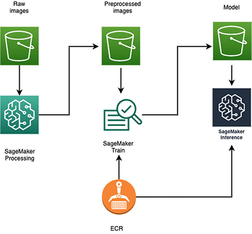
Data preprocessing using SageMaker Processing
The SVS slide images are preprocessed in three steps:
- Tiling images – The images are tiled by non-overlapping 512×512 pixel windows, and tiles containing over 50% background are discarded. The tiles are stored as JPEG images.
- Converting images to TFRecords – We use SageMaker Pipe mode to reduce our training time, which requires the data to be available in a proto-buffer format. TFRecord is a popular proto-buffer format used for training models with TensorFlow. We explain SageMaker Pipe mode and proto-buffer format in more detail in the following section.
- Sorting TFRecords – We sort the dataset into test, train, and validation cohorts for a three-way classifier (LUAD/LUSC/Normal). The TCGA dataset can have multiple slide images corresponding to a single patient. We need to make sure all the tiles generated from slides corresponding to the same patient occupy the same split to avoid data leakage. For the test set, we create per-slide TFRecord containing all the tiles from that slide so that we can evaluate the model in the way it will be used in deployment.
The following is the preprocessing code:
def generate_tf_records(base_folder, input_files, output_file, n_image, slide=None):
    record_file = output_file

    count = n_image
    with tf.io.TFRecordWriter(record_file) as writer:
        while count:
            filename, label = random.choice(input_files)
            temp_img = plt.imread(os.path.join(base_folder, filename))
            if temp_img.shape != (512, 512, 3):
                continue
            count -= 1

            image_string = np.float32(temp_img).tobytes()
            slide_string = slide.encode('utf-8') if slide else None
            tf_example = image_example(image_string, label, slide_string)
            writer.write(tf_example.SerializeToString())
We use SageMaker Processing for the preceding preprocessing steps, which allows us to run data preprocessing or postprocessing, feature engineering, data validation, and model evaluation workloads with SageMaker. Processing jobs accept data from Amazon S3 as input and store processed output data back into Amazon S3.
A benefit of using SageMaker Processing is the ease of distributing inputs across multiple compute instances. We can simply set s3_data_distribution_type=ShardedByS3Key parameter to divide data equally among all processing containers.
Importantly, the number of processing instances matches the number of GPUs we will use for distributed training with Horovod (i.e., 16). The reasoning becomes clearer when we introduce Horovod training.
The processing script is available on GitHub.
processor = Processor(image_uri=image_name,
                      role=get_execution_role(),
                      instance_count=16,               # run the job on 16 instances
                      base_job_name='processing-base', # should be unique name
                      instance_type='ml.m5.4xlarge',
                      volume_size_in_gb=1000)

processor.run(inputs=[ProcessingInput(
    source=f's3://<bucket_name>/tcga-svs', # s3 input prefix
    s3_data_type='S3Prefix',
    s3_input_mode='File',
    s3_data_distribution_type='ShardedByS3Key', # Split the data across instances
    destination='/opt/ml/processing/input')], # local path on the container
    outputs=[ProcessingOutput(
        source='/opt/ml/processing/output', # local output path on the container
        destination=f's3://<bucket_name>/tcga-svs-tfrecords/' # output s3 location
    )],
    arguments=['10000'], # number of tiled images per TF record for training dataset
    wait=True,
    logs=True)
Distributed model training using SageMaker Training
Taking ML models from conceptualization to production is typically complex and time-consuming. We have to manage large amounts of data to train the model, choose the best algorithm for training it, manage the compute capacity while training it, and then deploy the model into a production environment. SageMaker reduces this complexity by making it much easier to build and deploy ML models. It manages the underlying infrastructure to train your model at petabyte scale and deploy it to production.
After we preprocess the whole-slide images, we still have hundreds of gigabytes of data. Training on a single instance (GPU or CPU) would take several days or weeks to finish. To speed things up, we need to distribute the workload of training a model across multiple instances. For this post, we focus on distributed deep learning based on data parallelism using Horovod, a distributed training framework, and SageMaker Pipe mode.
Horovod: A cross-platform distributed training framework
When training a model with a large amount of data, the data needs to distributed across multiple CPUs or GPUs on either a single instance or multiple instances. Deep learning frameworks provide their own methods to support distributed training. Horovod is a popular framework-agnostic toolkit for distributed deep learning. It utilizes an allreduce algorithm for fast distributed training (compared with a parameter server approach) and includes multiple optimization methods to make distributed training faster. For more examples of distributed training with Horovod on SageMaker, see Multi-GPU and distributed training using Horovod in Amazon SageMaker Pipe mode and Reducing training time with Apache MXNet and Horovod on Amazon SageMaker.
SageMaker Pipe mode
You can provide input to SageMaker in either File mode or Pipe mode. In File mode, the input files are copied to the training instance. With Pipe mode, the dataset is streamed directly to your training instances. This means that the training jobs start sooner, compute and download can happen in parallel, and less disk space is required. Therefore, we recommend Pipe mode for large datasets.
SageMaker Pipe mode requires data to be in a protocol buffer format. Protocol buffers are language-neutral, platform-neutral, extensible mechanisms for serializing structured data. TFRecord is a popular proto-buffer format used for training models with TensorFlow. TFRecords are optimized for use with TensorFlow in multiple ways. First, they make it easy to combine multiple datasets and integrate seamlessly with the data import and preprocessing functionality provided by the library. Second, you can store sequence data—for instance, a time series or word encodings—in a way that allows for very efficient and (from a coding perspective) convenient import of this type of data.
The following diagram illustrates data access with Pipe mode.
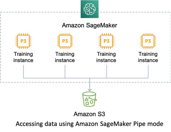
Data sharding with SageMaker Pipe mode
You should keep in mind a few considerations when working with SageMaker Pipe mode and Horovod:
- The data that is streamed through each pipe is mutually exclusive of the other pipes. The number of pipes dictates the number of data shards that need to be created.
- Horovod wraps the training script for each compute instance. This means that data for each compute instance needs to be from a different shard.
- With the SageMaker Training parameter
S3DataDistributionTypeset toShardedByS3Key, we can share a pipe with more than one instance. The data is streamed in round-robin fashion across instances.
To illustrate this better, let’s say we use two instances (A and B) of type ml.p3.8xlarge. Each ml.p3.8xlarge instance has four GPUs. We create four pipes (P1, P2, P3, and P4) and set S3DataDistributionType = 'ShardedByS3Key’. As shown in the following table, each pipe equally distributes the data between two instances in a round-robin fashion. This is the core concept needed in setting up pipes with Horovod. Because Horovod wraps the training script for each GPU, we need to create as many pipes as there are GPUs per training instance.
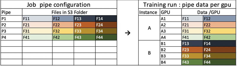
The following code shards the data in Amazon S3 for each pipe. Each shard should have a separate prefix in Amazon S3.
# Definite distributed training hyperparameters
train_instance_type='ml.p3.8xlarge'
train_instance_count = 4
gpus_per_host = 4
num_of_shards = gpus_per_host * train_instance_count

distributions = {'mpi': {
    'enabled': True,
    'processes_per_host': gpus_per_host
    }
}
# Sharding
client = boto3.client('s3')
result = client.list_objects(Bucket=s3://<bucket_name>, Prefix='tcga-svs-tfrecords/train/', Delimiter='/')

j = -1
for i in range(num_of_shards):
    copy_source = {
        'Bucket': s3://<bucket_name>,
        'Key': result['Contents'][i]['Key']
     }
    print(result['Contents'][i]['Key'])
    if i % gpus_per_host == 0:
        j += 1
    dest = 'tcga-svs-tfrecords/train_sharded/' + str(j) +'/' + result['Contents'][i]['Key'].split('/')[2]
    print(dest)
    s3.meta.client.copy(copy_source, s3://<bucket_name>, dest)


# Define inputs to SageMaker estimator
svs_tf_sharded = f's3://<bucket_name>/tcga-svs-tfrecords'
shuffle_config = sagemaker.session.ShuffleConfig(234)
train_s3_uri_prefix = svs_tf_sharded
remote_inputs = {}

for idx in range(gpus_per_host):
    train_s3_uri = f'{train_s3_uri_prefix}/train_sharded/{idx}/'
    train_s3_input = s3_input(train_s3_uri, distribution ='ShardedByS3Key', shuffle_config=shuffle_config)
    remote_inputs[f'train_{idx}'] = train_s3_input
    remote_inputs['valid_{}'.format(idx)] = '{}/valid'.format(svs_tf_sharded)
remote_inputs['test'] = '{}/test'.format(svs_tf_sharded)
remote_inputs
We use a SageMaker estimator to launch training on four instances of ml.p3.8xlarge. Each instance has four GPUs. Thus, there are a total of 16 GPUs. See the following code:
local_hyperparameters = {'epochs': 5, 'batch-size' : 16, 'num-train':160000, 'num-val':8192, 'num-test':8192}

estimator_dist = TensorFlow(base_job_name='svs-horovod-cloud-pipe',
                            entry_point='src/train.py',
                            role=role,
                            framework_version='2.1.0',
                            py_version='py3',
                            distribution=distributions,
                            volume_size=1024,
                            hyperparameters=local_hyperparameters,
                            output_path=f's3://<bucket_name>/output/',
                            instance_count=4,
                            instance_type=train_instance_type,
                            input_mode='Pipe')

estimator_dist.fit(remote_inputs, wait=True)
The following code snippet of the training script shows how to orchestrate Horovod with TensorFlow for distributed training:
mpi = False
if 'sagemaker_mpi_enabled' in args.fw_params:
    if args.fw_params['sagemaker_mpi_enabled']:
        import horovod.keras as hvd
        mpi = True
        # Horovod: initialize Horovod.
        hvd.init()
        # Pin GPU to be used to process local rank (one GPU per process)
        gpus = tf.config.experimental.list_physical_devices('GPU')
        tf.config.experimental.set_visible_devices(gpus[hvd.local_rank()], 'GPU')
else:
    hvd = None

callbacks = []
if mpi:
    callbacks.append(hvd.callbacks.BroadcastGlobalVariablesCallback(0))
    callbacks.append(hvd.callbacks.MetricAverageCallback())
    if hvd.rank() == 0:
        callbacks.append(ModelCheckpoint(args.output_dir + '/checkpoint-{epoch}.ckpt',
                                        save_weights_only=True,
                                        verbose=2))
else:
    callbacks.append(ModelCheckpoint(args.output_dir + '/checkpoint-{epoch}.ckpt',
                                    save_weights_only=True,
                                    verbose=2))

train_dataset = train_input_fn(hvd, mpi)
valid_dataset = valid_input_fn(hvd, mpi)
test_dataset = test_input_fn()
model = model_def(args.learning_rate, mpi, hvd)
logging.info("Starting training")
size = 1
if mpi:
    size = hvd.size()

model.fit(train_dataset,
          steps_per_epoch=((args.num_train // args.batch_size) // size),
          epochs=args.epochs,
          validation_data=valid_dataset,
          validation_steps=((args.num_val // args.batch_size) // size),
          callbacks=callbacks,
          verbose=2)
Because Pipe mode streams the data to each of our instances, the training script cannot calculate the data size during training (which is needed to compute steps_per_epoch). The parameter is therefore provided manually as a hyperparameter to the TensorFlow estimator. Additionally, the number of data points must be specified so that it can be divided equally amongst the GPUs. An unequal division could lead to a Horovod deadlock, because the time taken by each GPU to complete the training process is no longer identical. To ensure that the data points are equally divided, we use the same of number of instances for preprocessing as the number of GPUs for training. In our example, this number is 16.
Inference and deployment
After we train the model using SageMaker, we deploy it for inference on new images. To set up a persistent endpoint to get one prediction at a time, use SageMaker hosting services. To get predictions for an entire dataset, use SageMaker batch transform.
In this post, we deploy the trained model as a SageMaker endpoint. The following code deploys the model to an m4 instance, reads tiled image data from TFRecords, and generates a slide-level prediction:
# Generate predictor object from trained model
predictor = estimator_dist.deploy(initial_instance_count=1,
                                  instance_type='ml.m4.xlarge')

# Tile-level prediction
raw_image_dataset = tf.data.TFRecordDataset(f'images/{local_file}') # read a TFrecord
parsed_image_dataset = raw_image_dataset.map(dataset_parser) # Parse TFrecord to JPEGs

pred_scores_list = []
for i, element in enumerate(parsed_image_dataset):
    image = element[0].numpy()
    label = element[1].numpy()
    slide = element[2].numpy().decode()
    if i == 0:
        print(f"Making tile-level predictions for slide: {slide}...")

    print(f"Querying endpoint for a prediction for tile {i+1}...")
    pred_scores = predictor.predict(np.expand_dims(image, axis=0))['predictions'][0]
    pred_class = np.argmax(pred_scores)

    if i > 0 and i % 10 == 0:
        plt.figure()
        plt.title(f'Tile {i} prediction: {pred_class}')
        plt.imshow(image / 255)

    pred_scores_list.append(pred_scores)
print("Done.")

# Slide-level prediction (average score over all tiles)
mean_pred_scores = np.mean(np.vstack(pred_scores_list), axis=0)
mean_pred_class = np.argmax(mean_pred_scores)
print(f"Slide-level prediction for {slide}:", mean_pred_class)
The model is trained on individual tile images. During inference, the SageMaker endpoint provides classification scores for each tile. These scores are averaged out across all tiles to generate the slide-level score and prediction. The following diagram illustrates this workflow.
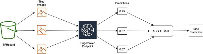
A majority vote scheme would also be appropriate.
To perform inference on a large new batch of slide images, you can run a batch transform job for offline predictions on the dataset in Amazon S3 on multiple instances. Once the processed TFRecords are retrieved from Amazon S3, you can replicate the preceding steps to generate a slide-level classification for each of the new images.
Conclusion
In this post, we introduced a scalable machine learning pipeline for ultra high-resolution images that uses SageMaker Processing, SageMaker Pipe mode, and Horovod. The pipeline simplifies the convoluted process of large-scale training of a classifier over a dataset consisting of images that approach the gigapixel scale. With SageMaker and Horovod, we eased the process by distributing inputs across multiple compute instances, which reduces training time. We also provided a simple but effective strategy to aggregate tile-level predictions to produce slide-level inference.
For more information about SageMaker, see Build, train, and deploy a machine learning model with Amazon SageMaker. For the complete example to run on SageMaker, in which Pipe mode and Horovod are applied together, see the GitHub repo.
References
- Nicolas Coudray, Paolo Santiago Ocampo, Theodore Sakellaropoulos, Navneet Narula, Matija Snuderl, David Fenyö, Andre L. Moreira, Narges Razavian, Aristotelis Tsirigos. “Classification and mutation prediction from non–small cell lung cancer histopathology images using deep learning”. Nature Medicine, 2018; DOI: 10.1038/s41591-018-0177-5
- https://github.com/ncoudray/DeepPATH/tree/master/DeepPATH_code
- https://www.cancer.gov/about-nci/organization/ccg/research/structural-genomics/tcga
About the Authors
 Karan Sindwani is a Data Scientist at Amazon Machine Learning Solutions where he builds and deploys deep learning models. He specializes in the area of computer vision. In his spare time, he enjoys hiking.
 Vinay Hanumaiah is a Deep Learning Architect at Amazon ML Solutions Lab, where he helps customers build AI and ML solutions to accelerate their business challenges. Prior to this, he contributed to the launch of AWS DeepLens and Amazon Personalize. In his spare time, he enjoys time with his family and is an avid rock climber.
 Ryan Brand is a Data Scientist in the Amazon Machine Learning Solutions Lab. He has specific experience in applying machine learning to problems in healthcare and the life sciences, and in his free time he enjoys reading history and science fiction.
 Tatsuya Arai, Ph.D. is a biomedical engineer turned deep learning data scientist on the Amazon Machine Learning Solutions Lab team. He believes in the true democratization of AI and that the power of AI shouldn’t be exclusive to computer scientists or mathematicians.