The Roaring 20+: GFN Thursday Game Releases Include Biomutant, Maneater, Warhammer Age of Sigmar: Storm Ground and More

GFN Thursday comes roaring in with 22 games and support for three DLCs joining the GeForce NOW library this week.

Among the 22 new releases are five day-and-date game launches: Biomutant, Maneater, King of Seas, Imagine Earth and Warhammer Age of Sigmar: Storm Ground.

DLC, Without the Download

GeForce NOW ensures your favorite games are automatically up to date, avoiding game updates and patches. Simply log in, click PLAY and enjoy an optimal cloud gaming experience.

This includes supporting the latest expansions and other downloadable content — without any local downloads.

Three great games are getting new DLC, and they’re streaming on GeForce NOW.

Hunt: Showdown - The Committed on GeForce NOW
Hunt: Showdown’s newest DLC adds new hunter Henry Monroe to the mix. He doesn’t look stable to us.

Hunt Showdown — The Committed DLC contains one Legendary Hunter (Monroe), a Legendary knife (Pane) and a Legendary Romero 77 (Lock and Key). It’s available on Steam, so members can start hunting now.

Isle of Siptah, the massive expansion to the open world survival game Conan Exiles, is exiting early access and releasing on Steam today. It features a vast new island to explore, huge and vile new creatures to slay, new building sets and a host of new features. Gamers have 40 new NPC camps and points of interest to explore, three new factions of NPCs, new ways of acquiring thralls and much more.

Announced last month, Iron Harvest – Operation Eagle, the new expansion to the critically acclaimed world of Iron Harvest set in the alternate reality of 1920, is available on Steam and streaming with GeForce NOW. Guide the new faction through seven new single-player missions, while learning how to use the game’s new Aircraft units across all of the game’s playable factions, including Polania, Saxony and Rusviet.

Newest Additions of the Week

GFN Thursday wouldn’t be complete without new games. The library evolved this week, but didn’t chew you up, with five day-and-date releases, including the launch of Biomutant, from Experiment 101 and THQ Nordic.

Biomutant is now available on GeForce NOW
A gorgeous open world to explore as a weapon-wielding rodent? That’s our perfect weekend.

Biomutant (Steam)

Explore a strange new world as an ever-evolving, weapon-wielding, martial arts master anthropomorphic rodent in this featured game of the week! For more information, read here

Including Biomutant, members can expect a total of 22 games this week:

May Games Update

A few games that we planned to release in May didn’t quite make it this month. Some were due to technical issues, others are on the way. Look for updates to the below in the weeks ahead.

  • Beyond Good & Evil (Steam)
  • Child of Light (Russian version only, Ubisoft Connect)
  • Hearts of Iron III (Steam)
  • King’s Bounty: Dark Side (Steam)
  • Sabotaj (Steam)
  • Super Mecha Champions (Steam)
  • Thea: The Awakening (Steam)
  • Tomb Raider Legend (Steam)

What are you going to play? Let us know on Twitter or in the comments below.

The post The Roaring 20+: GFN Thursday Game Releases Include Biomutant, Maneater, Warhammer Age of Sigmar: Storm Ground and More appeared first on The Official NVIDIA Blog.

Read More

Cross-Modal Contrastive Learning for Text-to-Image Generation

Posted by Han Zhang, Research Scientist and Jing Yu Koh, Software Engineer, Google Research

Automatic text-to-image synthesis, in which a model is trained to generate images from text descriptions alone, is a challenging task that has recently received significant attention. Its study provides rich insights into how machine learning (ML) models capture visual attributes and relate them to text. Compared to other kinds of inputs to guide image creation, such as sketches, object masks or mouse traces (which we have highlighted in prior work), descriptive sentences are a more intuitive and flexible way to express visual concepts. Hence, a strong automatic text-to-image generation system can also be a useful tool for rapid content creation and could be applied to many other creative applications, similar to other efforts to integrate machine learning into the creation of art (e.g., Magenta).

State-of-the-art image synthesis results are typically achieved using generative adversarial networks (GANs), which train two models — a generator, which tries to create realistic images, and a discriminator, which tries to determine if an image is real or fabricated. Many text-to-image generation models are GANs that are conditioned using text inputs in order to generate semantically relevant images. This is significantly challenging, especially when long, ambiguous descriptions are provided. Moreover, GAN training can be prone to mode collapse, a common failure case for the training process in which the generator learns to produce only a limited set of outputs, so that the discriminator fails to learn robust strategies to recognize fabricated images. To mitigate mode collapse, some approaches use multi-stage refinement networks that iteratively refine an image. However, such systems require multi-stage training, which is less efficient than simpler single-stage end-to-end models. Other efforts rely on hierarchical approaches that first model object layouts before finally synthesizing a realistic image. This requires the use of labeled segmentation data, which can be difficult to obtain.

In “Cross-Modal Contrastive Learning for Text-to-Image Generation,” to appear at CVPR 2021, we present the Cross-Modal Contrastive Generative Adversarial Network (XMC-GAN), which addresses text-to-image generation by learning to maximize the mutual information between image and text using inter-modal (image-text) and intra-modal (image-image) contrastive losses. This approach helps the discriminator to learn more robust and discriminative features, so XMC-GAN is less prone to mode collapse even with one-stage training. Importantly, XMC-GAN achieves state-of-the-art performance with a simple one-stage generation, as compared to previous multi-stage or hierarchical approaches. It is end-to-end trainable, and only requires image-text pairs (as opposed to labeled segmentation or bounding box data).

Contrastive Losses for Text-to-Image Synthesis
The goal of text-to-image synthesis systems is to produce clear, photo-realistic scenes with high semantic fidelity to their conditioned text descriptions. To achieve this, we propose to maximize the mutual information between the corresponding pairs: (1) images (real or generated) with a sentence describing the scene; (2) a generated image and a real image with the same description; and (3) regions of an image (real or generated) and words or phrases associated with them.

In XMC-GAN, this is enforced using contrastive losses. Similar to other GANs, XMC-GAN contains a generator for synthesizing images, and a discriminator that is trained to act as a critic between real and generated images. Three sets of data contribute to the contrastive loss in this system — the real images, the text that describes those images, and the images generated from the text descriptions. The individual loss functions for both the generator and the discriminator are combinations of the loss calculated from whole images with the full text description, combined with the loss calculated from sub-divided images with associated words or phrases. Then, for each batch of training data, we calculate the cosine similarity score between each text description and the real images, and likewise, between each text description and the batch of generated images. The goal is for the matching pairs (both text-to-image and real image-to-generated image) to have high similarity scores and for non-matching pairs to have low scores. Enforcing such a contrastive loss allows the discriminator to learn more robust and discriminative features.

Inter-modal and intra-modal contrastive learning in our proposed XMC-GAN text-to-image synthesis model.

Results
We apply XMC-GAN to three challenging datasets — the first was a collection of MS-COCO descriptions of MS-COCO images, and the other two were datasets annotated with Localized Narratives, one of which covers MS-COCO images (which we call LN-COCO) and the other of which describes Open Images data (LN-OpenImages). We find that XMC-GAN achieves a new state of the art on each. The images generated by XMC-GAN depict scenes that are of higher quality than those generated using other techniques. On MS-COCO, XMC-GAN improves the state-of-the-art Fréchet inception distance (FID) score from 24.7 to 9.3, and is significantly preferred by human evaluators.

Selected qualitative results for generated images on MS-COCO.

Similarly, human raters prefer the image quality in XMC-GAN generated images 77.3% of the time, and 74.1% prefer its image-text alignment compared to three other state-of-the-art approaches (CP-GAN, SD-GAN, and OP-GAN) .

Human evaluation on MS-COCO for image quality and text alignment. Annotators rank (anonymized and order-randomized) generated images from best to worst.

XMC-GAN also generalizes well to the challenging Localized Narratives dataset, which contains longer and more detailed descriptions. Our prior work TReCS tackles text-to-image generation for Localized Narratives using mouse trace inputs to improve image generation quality. Despite not receiving mouse trace annotations, XMC-GAN is able to significantly outperform TReCS on image generation on LN-COCO, improving state-of-the-art FID from 48.7 to 14.1. Incorporating mouse traces and other additional inputs into an end-to-end model such as XMC-GAN would be interesting to study in future work.

In addition, we also train and evaluate on the LN-OpenImages, which is more challenging than MS-COCO because the dataset is much larger with images that cover a broader range of subject matter and that are more complex (8.4 objects on average). To the best of our knowledge, XMC-GAN is the first text-to-image synthesis model that is trained and evaluated on Open Images. XMC-GAN is able to generate high quality results, and sets a strong benchmark FID score of 26.9 on this very challenging task.

Random samples of real and generated images on Open Images.

Conclusion and Future Work
In this work, we present a cross-modal contrastive learning framework to train GAN models for text-to-image synthesis. We investigate several cross-modal contrastive losses that enforce correspondence between image and text. For both human evaluations and quantitative metrics, XMC-GAN establishes a marked improvement over previous models on multiple datasets. It generates high quality images that match their input descriptions well, including for long, detailed narratives, and does so while being a simpler, end-to-end model. We believe that this represents a significant advance towards creative applications for image generation from natural language descriptions. As we continue this research, we are continually evaluating responsible approaches, potential applications and risk mitigation, in accordance with our AI Principles.

Acknowledgements
This is a joint work with Jason Baldridge, Honglak Lee, and Yinfei Yang. We would like to thank Kevin Murphy, Zizhao Zhang, Dilip Krishnan for their helpful feedback. We also want to thank the Google Data Compute team for their work on conducting human evaluations. We are also grateful for general support from the Google Research team.

Read More

OpenAI Startup Fund

OpenAI Startup Fund

The OpenAI Startup Fund is investing $100 million to help AI companies have a profound, positive impact on the world. We’re looking to partner with a small number of early-stage startups in fields where artificial intelligence can have a transformative effect—like health care, climate change, and education—and where AI tools can empower people by helping them be more productive.

The fund is managed by OpenAI, with investment from Microsoft and other OpenAI partners. In addition to capital, companies in the OpenAI Startup Fund will get early access to future OpenAI systems, support from our team, and credits on Azure.

If your startup plans to push the boundaries of today’s artificial intelligence by building with our API, we want to hear from you. Founders from underrepresented groups are especially encouraged to apply.

Please read our Privacy Policy and Terms of Use.

OpenAI

Run Your First Multi-Worker TensorFlow Training Job With GCP AI Platform

Posted by Nikita Namjoshi, Machine Learning Solutions Engineer

TensorFlow Header

When a single machine is not enough, it’s time to train and iterate faster with TensorFlow’s MultiWorkerMirroredStrategy. In this tutorial-style article you’ll learn how to launch a multi-worker training job on Google Cloud Platform (GCP) using AI Platform Training. You’ll also learn the basics of how TensorFlow distributes data and implements synchronous data parallelism across multiple machines. While this article focuses on a managed solution on GCP, you can also do all of this entirely in open-source on your own hardware.

Overview of Distributed Training

If you have a single GPU, TensorFlow will use this accelerator to speed up model training with no extra work on your part. However, if you want to get an additional boost from using multiple GPUs on a single machine or multiple machines (each with potentially multiple GPUs), then you’ll need to use tf.distribute, which is TensorFlow’s library for running a computation across multiple devices.

The simplest way to get started with distributed training is a single machine with multiple GPU devices. A TensorFlow distribution strategy from the tf.distribute module will manage the coordination of data distribution and gradient updates across all of the GPUs. If you want to learn more about training in this scenario, check out the previous post on distributed training basics.

If you’ve mastered single host training and are looking to scale even further, then adding multiple machines to your cluster can help you get an even greater performance boost. You can make use of a cluster of machines that are CPU only, or that each have one or more GPUs.

There are many ways to do multi-worker training on GCP. In this article we’ll use AI Platform Training, as it’s the quickest way to launch a distributed training job and has additional features that make it very easy to include as part of your production pipeline. To use this managed service, you’ll need to add a bit of extra code to your program and set up a config file that is specific to AI Platform. However; you will not have to endure the pains of GPU driver installation or cluster management, which can be very challenging in a distributed scenario.

Multi-Worker Cluster Configuration

The tf.distribute module currently provides two strategies for multi-worker training. In TensorFlow 2.5, ParameterServerStrategy is experimental, and MultiWorkerMirroredStrategy is a stable API.

Like its single-worker counterpart, MirroredStrategy, MultiWorkerMirroredStrategy is a synchronous data parallelism strategy that you can use with only a few code changes.

However, unlike MirroredStrategy, for a multi-worker setup TensorFlow needs to know which machines are part of your cluster. This is generally specified with the environment variable TF_CONFIG.

os.environ["TF_CONFIG"] = json.dumps({
"cluster": {
"chief": ["host1:port"],
"worker": ["host2:port", "host3:port"],
},
"task": {"type": "worker", "index": 1}
})

In this simple TF_CONFIG example, the “cluster” key contains a dictionary with the internal IPs and ports of all the machines. In MultiWorkerMirroredStrategy, all machines are designated as workers, which are the physical machines on which the replicated computation is executed. In addition to each machine being a worker, there needs to be one worker that takes on some extra work such as saving checkpoints and writing summary files to TensorBoard. This machine is known as the chief (or by its deprecated name master).

After you’ve added your machines to the cluster key, the next step is to set the “task”. This specifies the task type and task index of the current machine, which is an index into the cluster dictionary. The cluster key should be the same on each machine, but the task keys will be different.

Conveniently, when using AI Platform Training, the TF_CONFIG environment variable is set for you on each machine in your cluster so you don’t need to worry about this set up!

However, if you were trying to run a multi-worker job with, for example, 3 instances on Google Compute Engine, you would need to set this environment variable on each machine as shown below. For the machines that are not the chief, the TF_CONFIG looks the same except the task index increments by 1.

Machine 1 (Chief)

os.environ["TF_CONFIG"] = json.dumps({
"cluster": {
"chief": ["host1:port"],
"worker": ["host2:port", "host3:port"],
},
"task": {"type": "chief", "index": 0}
})

Machine 2

os.environ["TF_CONFIG"] = json.dumps({
"cluster": {
"chief": ["host1:port"],
"worker": ["host2:port", "host3:port"],
},
"task": {"type": "worker", "index": 0}
})

Machine 3

os.environ["TF_CONFIG"] = json.dumps({
"cluster": {
"chief": ["host1:port"],
"worker": ["host2:port", "host3:port"],
},
"task": {"type": "worker", "index": 1}
})

Setting this environment variable is fairly easy to do when you have only a few machines in your cluster; however, once you start scaling up, you don’t want to be assigning this variable to each machine manually. As mentioned earlier, one of the many benefits of using AI Platform is that this coordination happens automatically. The only configuration you have to provide is the number of machines in your cluster, and the number and type of GPUs per machine. We’ll do this step in a later section.

Set up the Distribution Strategy

In this Colab notebook, you’ll find the code to train a ResNet50 architecture on the Cassava dataset. In the following sections, we’ll review the new code that needs to be added to our program in order to do distributed training on multiple machines.

As with any strategy in the tf.distribute module, step one is to instantiate the strategy.

strategy = tf.distribute.MultiWorkerMirroredStrategy()

Note that there is a limitation where the instance of MultiWorkerMirroredStrategy needs to be created at the beginning of the program. Code that may create ops should be placed after the strategy is instantiated.

Next, you wrap the creation of your model variables within the strategy’s scope. This crucial step tells TensorFlow which variables should be mirrored across the replicas.

with strategy.scope():
model = create_model()
model.compile(
loss='sparse_categorical_crossentropy',
optimizer=tf.keras.optimizers.Adam(0.0001),
metrics=['accuracy'])

Lastly, you’ll need to scale your batch size by the number of replicas in your cluster. This ensures that each replica processes the same number of examples on each step.

per_replica_batch_size = 64
global_batch_size = per_replica_batch_size * strategy.num_replicas_in_sync

If you’ve used MirroredStrategy before, then the previous steps should be familiar. The main difference when moving from synchronous data parallelism on one machine to many is that the gradients at the end of each step now need to be synchronized across all GPUs in a machine and across all machines in the cluster. This additional step of synchronizing across the machines increases the overhead of distribution.

In TensorFlow, the multi-worker all-reduce communication is achieved via CollectiveOps. You don’t need to know much detail to execute a successful and performant training job, but at a high level, a collective op is a single op in the TensorFlow graph that can automatically choose an all-reduce algorithm according to factors such as hardware, network topology, and tensor sizes.

Dataset Sharding

In the single worker case, at each step your dataset is divided up across the replicas on your machine. This data splitting process becomes slightly more complicated in the multi-worker case. The data now also needs to be sharded, meaning that each worker is assigned a subset of the entire dataset. Therefore, at each step a global batch size of non overlapping dataset elements will be processed by each worker. This sharding happens automatically with tf.data.experimental.AutoShardPolicy.

By default, TensorFlow will first attempt to shard your data by FILE. This means that if your data exists across multiple files, each worker will process different file(s) and split the corresponding data amongst the replicas. FILE is the default autoshard policy because MultiWorkerMirroredStrategy works best for use cases with very large datasets, which are likely to not be in a single file. However, this option can lead to idle workers if the number of files is not divisible by the number of workers, or if some files are substantially longer than others.

If your data is not stored in multiple files, then the AutoShardPolicy will fall back to DATA, meaning that TensorFlow will autoshard the elements across all the workers. This guards against the potential idle worker scenario, but the downside is that the entire dataset will be read on each worker. You can read more about the different policies and see examples in the Distributed Input guide.

If you don’t want to use the default AUTO policy, you can set the desired AutoShardPolicy with the following code:

options = tf.data.Options()
options.experimental_distribute.auto_shard_policy = tf.data.experimental.AutoShardPolicy.DATA
train_data = train_data.with_options(options)

Save Your Model

Saving your model is slightly more complicated in the multi-worker case because the destination needs to be different for each of the workers. The chief worker will save to the desired model directory, while the other workers will save the model to temporary directories. It’s important that these temporary directories are unique in order to prevent multiple workers from writing to the same location. Saving can contain collective ops, so all workers must save and not just the chief.

The following is boilerplate code that implements the intended saving logic, as well as some cleanup to delete the temporary directories once the training has completed. Note that the model_path is the name of the Google Cloud Storage (GCS) bucket where your model will be saved at the end of training.

model_path = {gs://path_to_your_gcs_bucket}

# Note that with MultiWorkerMirroredStrategy,
# the program is run on every worker.
def _is_chief(task_type, task_id):
# Note: there are two possible `TF_CONFIG` configurations.
# 1) In addition to `worker` tasks, a `chief` task type is used.
# The implementation demonstrated here is for this case.
# 2) Only `worker` task type is used; in this case, worker 0 is
# regarded as the chief. In this case, this function
# should be modified to
# return (task_type == 'worker' and task_id == 0) or task_type is None
return task_type == 'chief'


def _get_temp_dir(dirpath, task_id):
base_dirpath = 'workertemp_' + str(task_id)
temp_dir = os.path.join(dirpath, base_dirpath)
tf.io.gfile.makedirs(temp_dir)
return temp_dir

def write_filepath(filepath, task_type, task_id):
dirpath = os.path.dirname(filepath)
base = os.path.basename(filepath)
if not _is_chief(task_type, task_id):
dirpath = _get_temp_dir(dirpath, task_id)
return os.path.join(dirpath, base)

# Determine type and task of the machine from
# the strategy cluster resolver
task_type, task_id = (strategy.cluster_resolver.task_type,
strategy.cluster_resolver.task_id)

# Based on the type and task, write to the desired model path
write_model_path = write_filepath(model_path, task_type, task_id)
model.save(write_model_path)

Everything we’ve covered about setting up the distribution strategy, sharding data, and saving models applies whether you’re training on GCP, your own hardware, or another cloud platform.

Prepare code for AI Platform

The basic prerequisites for using AI Platform are that you need to have a GCP project with billing enabled, the AI Platform APIs enabled, and sufficient AI Platform quota. If any of these steps are a mystery to you, refer to the previous post to get up to speed on GCP basics.

If you’re already familiar with training on AI Platform with a single node, then you’ll likely breeze through this section. We’ll take the pieces we walked through in the previous section, and do a bit of rearranging to match AI Platform Training convention. All of the code can be found in this Github repo, but we’ll walk through it in detail in this section.

By AI Platform convention, training code is arranged according to the diagram below. The task.py file contains the code that executes your training job. The example in this tutorial also includes a model.py file, which has the Keras functional API code for the model. For more complex production applications you’ll likely have additional util.py or setup.py files, and you can see where those fit in the hierarchy below.

diagram showing path of file

Model code

The model.py file can be found in Github here. You can see that this file just has the code for building the ResNet50 model architecture.

Task code

The task.py file can be found in Github here. This file contains the main function, which will execute the training job and save the model.

def main():
args = get_args()
strategy = tf.distribute.MultiWorkerMirroredStrategy()
global_batch_size = PER_REPLICA_BATCH_SIZE * strategy.num_replicas_in_sync
train_data, number_of_classes = create_dataset(global_batch_size)

with strategy.scope():
model = create_model(number_of_classes)

model.fit(train_data, epochs=args.epochs)

# Determine type and task of the machine from
# the strategy cluster resolver
task_type, task_id = (strategy.cluster_resolver.task_type,
strategy.cluster_resolver.task_id)

# Based on the type and task, write to the desired model path
write_model_path = write_filepath(args.job_dir, task_type, task_id)
model.save(write_model_path)

In this simple example, the data preprocessing happens directly in the task.py file, but in reality for more complicated data processing you would probably want to split out this code into a separate data.py file that you can import into task.py (for example if your preprocessing includes parsing TFRecord files).

We explicitly set the AutoShardPolicy to DATA in this case because the Cassava dataset is not downloaded as multiple files. However, if we did not set the policy to DATA, the default AUTO policy would kick in and the end result would be the same.

options = tf.data.Options()
options.experimental_distribute.auto_shard_policy = tf.data.experimental.AutoShardPolicy.DATA
train_data = train_data.with_options(options)

The task.py file also parses any command line arguments we need. In this simple example, the epochs are passed in via the command line. Additionally, we need to parse the argument job-dir, which is the GCS bucket where our model will be stored.

def get_args():
'''Parses args.'''
parser = argparse.ArgumentParser()
parser.add_argument(
'--epochs',
required=True,
type=int,
help='number training epochs')
parser.add_argument(
'--job-dir',
required=True,
type=str,
help='bucket to save model')
args = parser.parse_args()
return args

Lastly, the task.py file contains our boilerplate code for saving the model. For a production example, you probably would want to add this boilerplate to a util.py file, but again for this simple example we’ll keep everything in one file.

Custom Container Set up

AI Platform provides standard runtimes for you to execute your training job. While these runtimes might work for your use case, more specialized needs require a custom container. In this section, we’ll walk through how to set up your container image and push it to Google Container Registry (GCR).

Write Your Dockerfile

The following Dockerfile specifies the base image, using the TensorFlow 2.5 Enterprise GPU Deep Learning Container. Using the TensorFlow Enterprise image as our base image provides a useful design pattern for developing on GCP. TensorFlow Enterprise is a distribution of TensorFlow that is optimized for GCP. You can use TensorFlow Enterprise with AI Platform Notebooks, the Deep Learning VMs, and AI Platform Training, providing a seamless transition between different environments.

The code in our trainer directory is copied to the Docker image, and our entry point is the task.py script, which we will run as a module.

# Specifies base image and tag
FROM gcr.io/deeplearning-platform-release/tf2-gpu.2-5
WORKDIR /root

# Copies the trainer code to the docker image.
COPY trainer/ /root/trainer/

# Sets up the entry point to invoke the trainer.
ENTRYPOINT ["python", "-m", "trainer.task"]

Push Your Dockerfile to GCR

Next, we’ll set up some useful environment variables. You can select any name of your choosing for IMAGE_REPO_NAME and IMAGE_TAG. If you have not already set up the Google Cloud SDK, you can follow the steps here, as you’ll need to use the gcloud tool to push your container and kick off the training job.

export PROJECT_ID=$(gcloud config list project --format "value(core.project)")
export IMAGE_REPO_NAME={your_repo_name}
export IMAGE_TAG={your_image_tag}
export IMAGE_URI=gcr.io/$PROJECT_ID/$IMAGE_REPO_NAME:$IMAGE_TAG

Next, you’ll build your Dockerfile.

docker build -f Dockerfile -t $IMAGE_URI ./

Lastly, you can push your image to GCR.

gcloud auth configure-docker
docker push $IMAGE_URI

If you navigate to the GCR page in the GCP console UI, you should see your newly pushed image.

Configure Your Cluster

The final step before we can kick off our training job is to set up the cluster. AI Platform offers a set of predefined cluster specifications called scale tiers, but we’ll need to provide our own cluster setup for distributed training.

In the following config.yaml file, we’ve designated one master (equivalent to chief) and one worker. Each machine has one NVIDIA T4 Tensor Core GPU. For both machines, you’ll also need to specify the imageUri as the image you pushed to GCR in the previous step.

trainingInput:
scaleTier: CUSTOM
masterType: n1-standard-8
masterConfig:
acceleratorConfig:
count: 1
type: NVIDIA_TESLA_T4
imageUri: gcr.io/{path/to/image}:{tag}
useChiefInTfConfig: true
workerType: n1-standard-8
workerCount: 1
workerConfig:
acceleratorConfig:
count: 1
type: NVIDIA_TESLA_T4
imageUri: gcr.io/{path/to/image}:{tag}

In case you’re wondering what the useChiefInTfConfig flag does, TensorFlow uses the terminology “Chief” and AI Platform uses the terminology “Master”, so this flag will manage that discrepancy. You don’t need to worry about the details (although you will see an error message if you forget to set this flag!).

Feel free to experiment with this configuration by adding machines, adding GPUs, or removing all GPUs and training with CPUs only. You can see the supported regions and GPU types here for AI Platform, so just make sure your project has sufficient quota for whatever configuration you choose.

Launch Your Training Job

You can launch your training job easily with the following command:

gcloud ai-platform jobs submit training {job_name}  
--region europe-west2
--config config.yaml
--job-dir gs://{gcs_bucket/model_dir} --
--epochs 5

In the command above, you’ll need to give your job a name. In addition to passing in the region, you’ll need to define job-dir, which is the directory in your GCS bucket where you want your saved model file to be stored after training completes.

The empty — flag marks the end of the gcloud specific flags and the start of the args that you want to pass to your application (in this case, this is just the epochs).

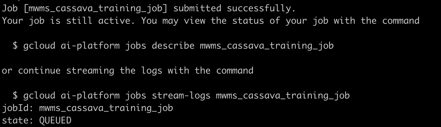
After executing the training command, you should see the following message.

code snippet

You can navigate to the AI Platform UI in the GCP console and track the status of your job.

You’ll notice that your job will take around ten minutes to launch. This overhead might seem huge in our simple example where it doesn’t even take ten minutes to train on a single GPU. However, this overhead will be amortized for large jobs.

job details screen

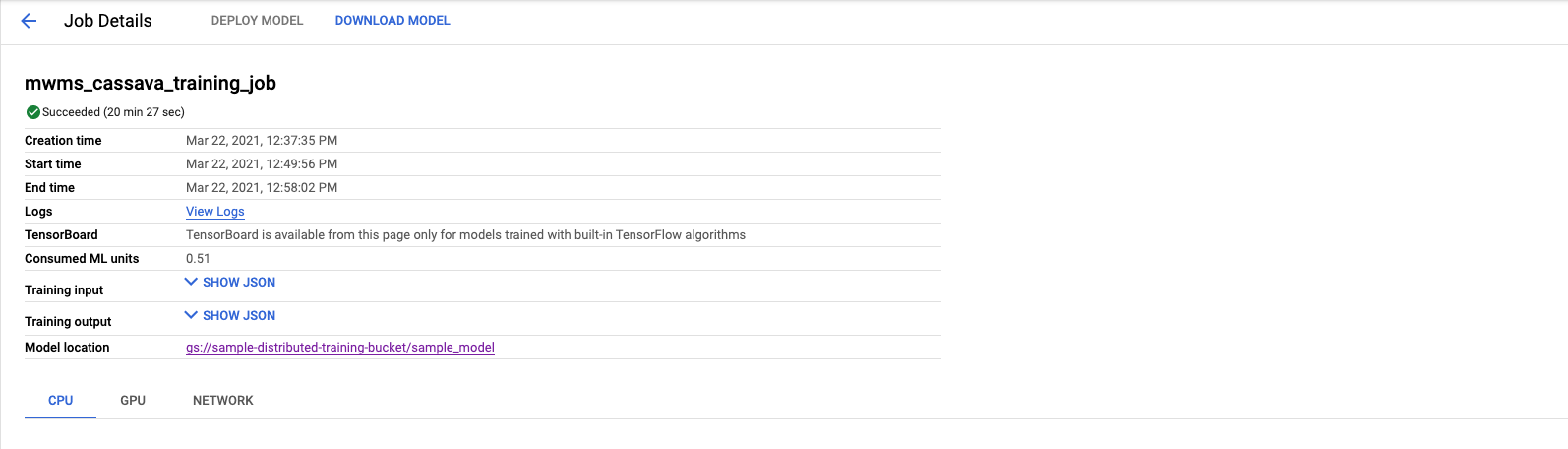
When the job completes training, you’ll see a green check mark next to the job. You can then click the Model location URI and you’ll find your saved_model.pb file.

What’s Next

You now know the basics of launching a multi-worker training job on GCP. You also know the core concepts of MultiWorkerMirroredStrategy. To take your skills to the next level, try leveraging AI Platform’s hyperparameter tuning feature for your next training job (in open-source, you can use Keras Tuner), or using TFRecord files as your input data. You can also try out Parameter Server Strategy if you’d like to explore asynchronous training in TensorFlow. Happy distributed training!

Read More

Gain valuable ML skills with the AWS Machine Learning Engineer Nanodegree Scholarship from Udacity

Amazon Web Services is partnering with Udacity to help educate developers of all skill levels on machine learning (ML) concepts with the AWS Machine Learning Scholarship Program by Udacity by offering 425 scholarships, with a focus on women and underrepresented groups.

Machine learning is an exciting and rapidly developing technology that has the power to create millions of jobs and transform our daily lives. According to the Future of Jobs Report 2020 by the World Economic Forum, by 2025, 97 million new roles may be created as a result of ML innovation. However, only today’s developers have the skills to act on these opportunities now. Proximity to high-quality education, cost of traditional education, and allocating time to start and complete new learning projects make learning ML more complicated.

To address this challenge, AWS invests in educating developers, data scientists, and ML developers with a variety of education solutions, such as exploring reinforcement learning concepts with AWS DeepRacer, training and validation with the AWS Certified Machine Learning – Specialty certification, and hands-on tutorials from the AWS Machine Learning Community.

Up-leveling ML skills and opening new career opportunities

With the AWS Machine Learning Engineer Nanodegree by Udacity, developers can learn valuable skills for ML career path with an interactive, cost-effective, and accessible ML education. All students that enroll in the scholarship program have access to AWS Machine Learning Foundations, a free course covering an introduction to ML concepts, including reinforcement learning, computer vision, and generative artificial intelligence, with expert-led interactive tutorials with AWS AI Devices such as AWS DeepRacer, AWS DeepLens, and AWS DeepComposer.

The AWS Machine Learning Scholarship Program is open to all for registration starting May 26, 2021, through June 23, 2021. Your learning journey begins with the free AWS Machine Learning Foundations course on June 28, 2021, in which you learn the fundamental aspects of ML, ML techniques and algorithms, programming best practices, Python coding, and interactive tutorials with AWS AI Devices. You have 3months to study and complete your assessment by October 11, 2021, with the top 425 students eligible for a scholarship to the AWS Machine Learning Engineer Nanodegree.

The AWS Machine Learning Foundations Course (free) includes the following objectives:

  • Learn the fundamentals of ML
  • Learn object-oriented programming best practices
  • Learn computer vision with AWS DeepLens, reinforcement learning with AWS DeepRacer, and generative AI with AWS DeepComposer.
  • Dedicate 3–5 hours a week on the course and work towards earning one of the follow-up Nanodegree program scholarships

In the Machine Learning Engineer Nanodegree program (a $1,000 value course), you learn advanced ML techniques and algorithms, including how to package and deploy models to a production environment.

The AWS Machine Learning Nanodegree Program enabled me to learn and achieve valuable machine learning skills at my own pace with interactive modules that made learning fun and effective,” said Juv Chan, AWS ML Hero and AWS Machine Learning Nanodegree Program Alumni. “Carving out time to learn machine learning can be very hard, especially under the demanding schedules that software engineers work from. The flexibility offered by Udacity Nanodegrees lets me learn new skills on a timetable that works for me.”

This year, we added 100 additional scholarships on top of the 325 scholarships allocated in 2020, and updated the content for students with advanced ML techniques and algorithms and expert-led tutorials on deploying ML models at scale with Amazon SageMaker.

AWS is also collaborating with several nonprofit organizations through the We Power Tech Program to increase the diversity and talent in technical roles, including organizations like Girls In Tech and the National Society of Black Engineers. As part of these ongoing relationships, the nonprofit organizations will help encourage women and underrepresented groups to participate in the AWS Machine Learning Engineer Nanodegree Scholarship Program. Organizations like these develop programs to inspire, support, train, and empower people from underrepresented groups to pursue careers in tech.

“AWS strives to help level the playing field for women and people of color, who have been underrepresented in the tech industry for far too long. We are thrilled to collaborate with Udacity to make this sort of technical training more widely available and accessible,” said LaDavia Drane, global head of Inclusion, Diversity & Equity at AWS. “We look forward to seeing the incredible innovations in machine learning that are sure to come from this initiative.”

“Tech needs representation from women, BIPOC, and other marginalized communities in every aspect of our industry. Companies must make meaningful and measurable change in the areas of diversity, equity, and inclusion to reach their greatest potential, and skills training programs uniquely tailored to increase representation from these groups are necessary for technology to achieve all that it’s capable of. Girls in Tech applauds our collaborator AWS, as well as Udacity, for breaking down the barriers that so often leave women behind in tech. Together, we aim to give everyone a seat at the table.” Adriana Gascoigne, Founder and CEO, Girls in Tech.

How the AWS Machine Learning Engineer Nanodegree Scholarship works

Scholarship enrollment is open from May 26, 2021, through June 23, 2021. Students begin their learning journey with the AWS Machine Learning Foundations Course from June 28, 2021, through October 11, 2021. At the end of the course, learners take an assessment, from which top students are selected for 425 scholarships, who then start the AWS Machine Learning Engineer Nanodegree from October 25, 2021, through January 25, 2022.

Get started and leverage the community

Get started by enrolling now and accelerate your ML journey! Connect with experts and like-minded aspiring ML developers on the AWS Machine Learning Slack channel.


About the Author

Cameron Peron is Senior Marketing Manager for AWS AI/ML Education and the AWS AI/ML community. He evangelizes how AI/ML innovation solves complex challenges facing community, enterprise, and startups alike. Out of the office, he enjoys staying active with kettlebell-sport, spending time with his family and friends, and is an avid fan of Euro-league basketball.

Read More

Everything you need to know about TorchVision’s MobileNetV3 implementation

In TorchVision v0.9, we released a series of new mobile-friendly models that can be used for Classification, Object Detection and Semantic Segmentation. In this article, we will dig deep into the code of the models, share notable implementation details, explain how we configured and trained them, and highlight important tradeoffs we made during their tuning. Our goal is to disclose technical details that typically remain undocumented in the original papers and repos of the models.

Network Architecture

The implementation of the MobileNetV3 architecture follows closely the original paper. It is customizable and offers different configurations for building Classification, Object Detection and Semantic Segmentation backbones. It was designed to follow a similar structure to MobileNetV2 and the two share common building blocks.

Off-the-shelf, we offer the two variants described on the paper: the Large and the Small. Both are constructed using the same code with the only difference being their configuration which describes the number of blocks, their sizes, their activation functions etc.

Configuration parameters

Even though one can write a custom InvertedResidual setting and pass it to the MobileNetV3 class directly, for the majority of applications we can adapt the existing configs by passing parameters to the model building methods. Some of the key configuration parameters are the following:

  • The width_mult parameter is a multiplier that affects the number of channels of the model. The default value is 1 and by increasing or decreasing it one can change the number of filters of all convolutions, including the ones of the first and last layers. The implementation ensures that the number of filters is always a multiple of 8. This is a hardware optimization trick which allows for faster vectorization of operations.

  • The reduced_tail parameter halves the number of channels on the last blocks of the network. This version is used by some Object Detection and Semantic Segmentation models. It’s a speed optimization which is described on the MobileNetV3 paper and reportedly leads to a 15% latency reduction without a significant negative effect on accuracy.

  • The dilated parameter affects the last 3 InvertedResidual blocks of the model and turns their normal depthwise Convolutions to Atrous Convolutions. This is used to control the output stride of these blocks and has a significant positive effect on the accuracy of Semantic Segmentation models.

Implementation details

Below we provide additional information on some notable implementation details of the architecture.
The MobileNetV3 class is responsible for building a network out of the provided configuration. Here are some implementation details of the class:

  • The last convolution block expands the output of the last InvertedResidual block by a factor of 6. The implementation is aligned with the Large and Small configurations described on the paper and can adapt to different values of the multiplier parameter.

  • Similarly to other models such as MobileNetV2, a dropout layer is placed just before the final Linear layer of the classifier.

The InvertedResidual class is the main building block of the network. Here are some notable implementation details of the block along with its visualization which comes from Figure 4 of the paper:

  • There is no expansion step if the input channels and the expanded channels are the same. This happens on the first convolution block of the network.

  • There is always a projection step even when the expanded channels are the same as the output channels.

  • The activation method of the depthwise block is placed before the Squeeze-and-Excite layer as this improves marginally the accuracy.

Classification

In this section we provide benchmarks of the pre-trained models and details on how they were configured, trained and quantized.

Benchmarks

Here is how to initialize the pre-trained models:

large = torchvision.models.mobilenet_v3_large(pretrained=True, width_mult=1.0,  reduced_tail=False, dilated=False)
small = torchvision.models.mobilenet_v3_small(pretrained=True)
quantized = torchvision.models.quantization.mobilenet_v3_large(pretrained=True)

Below we have the detailed benchmarks between new and selected previous models. As we can see MobileNetV3-Large is a viable replacement of ResNet50 for users who are willing to sacrifice a bit of accuracy for a roughly 6x speed-up:

Model Acc@1 Acc@5 Inference on CPU (sec) # Params (M)
MobileNetV3-Large 74.042 91.340 0.0411 5.48
MobileNetV3-Small 67.668 87.402 0.0165 2.54
Quantized MobileNetV3-Large 73.004 90.858 0.0162 2.96
MobileNetV2 71.880 90.290 0.0608 3.50
ResNet50 76.150 92.870 0.2545 25.56
ResNet18 69.760 89.080 0.1032 11.69

Note that the inference times are measured on CPU. They are not absolute benchmarks, but they allow for relative comparisons between models.

Training process

All pre-trained models are configured with a width multiplier of 1, have full tails, are non-dilated, and were fitted on ImageNet. Both the Large and Small variants were trained using the same hyper-parameters and scripts which can be found in our references folder. Below we provide details on the most notable aspects of the training process.

Achieving fast and stable training

Configuring RMSProp correctly was crucial to achieve fast training with numerical stability. The authors of the paper used TensorFlow in their experiments and in their runs they reported using quite high rmsprop_epsilon comparing to the default. Typically this hyper-parameter takes small values as it’s used to avoid zero denominators, but in this specific model choosing the right value seems important to avoid numerical instabilities in the loss.

Another important detail is that though PyTorch’s and TensorFlow’s RMSProp implementations typically behave similarly, there are a few differences with the most notable in our setup being how the epsilon hyperparameter is handled. More specifically, PyTorch adds the epsilon outside of the square root calculation while TensorFlow adds it inside. The result of this implementation detail is that one needs to adjust the epsilon value while porting the hyper parameter of the paper. A reasonable approximation can be taken with the formula PyTorch_eps = sqrt(TF_eps).

Increasing our accuracy by tuning hyperparameters & improving our training recipe

After configuring the optimizer to achieve fast and stable training, we turned into optimizing the accuracy of the model. There are a few techniques that helped us achieve this. First of all, to avoid overfitting we augmented out data using the AutoAugment algorithm, followed by RandomErasing. Additionally we tuned parameters such as the weight decay using cross validation. We also found beneficial to perform weight averaging across different epoch checkpoints after the end of the training. Finally, though not used in our published training recipe, we found that using Label Smoothing, Stochastic Depth and LR noise injection improve the overall accuracy by over 1.5 points.

The graph and table depict a simplified summary of the most important iterations for improving the accuracy of the MobileNetV3 Large variant. Note that the actual number of iterations done while training the model was significantly larger and that the progress in accuracy was not always monotonically increasing. Also note that the Y-axis of the graph starts from 70% instead from 0% to make the difference between iterations more visible:

Iteration Acc@1 Acc@5
Baseline with “MobileNetV2-style” Hyperparams 71.542 90.068
+ RMSProp with default eps 70.684 89.38
+ RMSProp with adjusted eps & LR scheme 71.764 90.178
+ Data Augmentation & Tuned Hyperparams 73.86 91.292
+ Checkpoint Averaging 74.028 91.382
+ Label Smoothing & Stochastic Depth & LR noise 75.536 92.368

Note that once we’ve achieved an acceptable accuracy, we verified the model performance on the hold-out test dataset which hasn’t been used before for training or hyper-parameter tuning. This process helps us detect overfitting and is always performed for all pre-trained models prior their release.

Quantization

We currently offer quantized weights for the QNNPACK backend of the MobileNetV3-Large variant which provides a speed-up of 2.5x. To quantize the model, Quantized Aware Training (QAT) was used. The hyper parameters and the scripts used to train the model can be found in our references folder.

Note that QAT allows us to model the effects of quantization and adjust the weights so that we can improve the model accuracy. This translates to an accuracy increase of 1.8 points comparing to simple post-training quantization:

Quantization Status Acc@1 Acc@5
Non-quantized 74.042 91.340
Quantized Aware Training 73.004 90.858
Post-training Quantization 71.160 89.834

Object Detection

In this section, we will first provide benchmarks of the released models, and then discuss how the MobileNetV3-Large backbone was used in a Feature Pyramid Network along with the FasterRCNN detector to perform Object Detection. We will also explain how the network was trained and tuned alongside with any tradeoffs we had to make. We will not cover details about how it was used with SSDlite as this will be discussed on a future article.

Benchmarks

Here is how the models are initialized:

high_res = torchvision.models.detection.fasterrcnn_mobilenet_v3_large_fpn(pretrained=T low_res = torchvision.models.detection.fasterrcnn_mobilenet_v3_large_320_fpn(pretraine

Below are some benchmarks between new and selected previous models. As we can see the high resolution Faster R-CNN with MobileNetV3-Large FPN backbone seems a viable replacement of the equivalent ResNet50 model for those users who are willing to sacrifice few accuracy points for a 5x speed-up:

Model mAP Inference on CPU (sec) # Params (M)
Faster R-CNN MobileNetV3-Large FPN (High-Res) 32.8 0.8409 19.39
Faster R-CNN MobileNetV3-Large 320 FPN (Low-Res) 22.8 0.1679 19.39
Faster R-CNN ResNet-50 FPN 37.0 4.1514 41.76
RetinaNet ResNet-50 FPN 36.4 4.8825 34.01

Implementation details

The Detector uses a FPN-style backbone which extracts features from different convolutions of the MobileNetV3 model. By default the pre-trained model uses the output of the 13th InvertedResidual block and the output of the Convolution prior to the pooling layer but the implementation supports using the outputs of more stages.

All feature maps extracted from the network have their output projected down to 256 channels by the FPN block as this greatly improves the speed of the network. These feature maps provided by the FPN backbone are used by the FasterRCNN detector to provide box and class predictions at different scales.

Training & Tuning process

We currently offer two pre-trained models capable of doing object detection at different resolutions. Both models were trained on the COCO dataset using the same hyper-parameters and scripts which can be found in our references folder.

The High Resolution detector was trained with images of 800-1333px, while the mobile-friendly Low Resolution detector was trained with images of 320-640px. The reason why we provide two separate sets of pre-trained weights is because training a detector directly on the smaller images leads to a 5 mAP increase in precision comparing to passing small images to the pre-trained high-res model. Both backbones were initialized with weights fitted on ImageNet and the 3 last stages of their weights where fined-tuned during the training process.

An additional speed optimization can be applied on the mobile-friendly model by tuning the RPN NMS thresholds. By sacrificing only 0.2 mAP of precision we were able to improve the CPU speed of the model by roughly 45%. The details of the optimization can be seen below:

Tuning Status mAP Inference on CPU (sec)
Before 23.0 0.2904
After 22.8 0.1679

Below we provide some examples of visualizing the predictions of the Faster R-CNN MobileNetV3-Large FPN model:

Semantic Segmentation

In this section we will start by providing some benchmarks of the released pre-trained models. Then we will discuss how a MobileNetV3-Large backbone was combined with segmentation heads such as LR-ASPP, DeepLabV3 and the FCN to conduct Semantic Segmentation. We will also explain how the network was trained and propose a few optional optimization techniques for speed critical applications.

Benchmarks

This is how to initialize the pre-trained models:

lraspp = torchvision.models.segmentation.lraspp_mobilenet_v3_large(pretrained=True) deeplabv3 = torchvision.models.segmentation.deeplabv3_mobilenet_v3_large(pretrained=Tr

Below are the detailed benchmarks between new and selected existing models. As we can see, the DeepLabV3 with a MobileNetV3-Large backbone is a viable replacement of FCN with ResNet50 for the majority of applications as it achieves similar accuracy with a 8.5x speed-up. We also observe that the LR-ASPP network supersedes the equivalent FCN in all metrics:

Model mIoU Global Pixel Acc Inference on CPU (sec) # Params (M)
LR-ASPP MobileNetV3-Large 57.9 91.2 0.3278 3.22
DeepLabV3 MobileNetV3-Large 60.3 91.2 0.5869 11.03
FCN MobileNetV3-Large (not released) 57.8 90.9 0.3702 5.05
DeepLabV3 ResNet50 66.4 92.4 6.3531 39.64
FCN ResNet50 60.5 91.4 5.0146 32.96

Implementation details

In this section we will discuss important implementation details of tested segmentation heads. Note that all models described in this section use a dilated MobileNetV3-Large backbone.

LR-ASPP

The LR-ASPP is the Lite variant of the Reduced Atrous Spatial Pyramid Pooling model proposed by the authors of the MobileNetV3 paper. Unlike the other segmentation models in TorchVision, it does not make use of an auxiliary loss. Instead it uses low and high-level features with output strides of 8 and 16 respectively.

Unlike the paper where a 49×49 AveragePooling layer with variable strides is used, our implementation uses an AdaptiveAvgPool2d layer to process the global features. This is because the authors of the paper tailored the head to the Cityscapes dataset while our focus is to provide a general purpose implementation that can work on multiple datasets. Finally our implementation always has a bilinear interpolation before returning the output to ensure that the sizes of the input and output images match exactly.

DeepLabV3 & FCN

The combination of MobileNetV3 with DeepLabV3 and FCN follows closely the ones of other models and the stage estimation for these methods is identical to LR-ASPP. The only notable difference is that instead of using high and low level features, we attach the normal loss to the feature map with output stride 16 and an auxiliary loss on the feature map with output stride 8.

Finally we should note that the FCN version of the model was not released because it was completely superseded by the LR-ASPP both in terms of speed and accuracy. The pre-trained weights are still available and can be used with minimal changes to the code.

Training & Tuning process

We currently offer two MobileNetV3 pre-trained models capable of doing semantic segmentation: the LR-ASPP and the DeepLabV3. The backbones of the models were initialized with ImageNet weights and trained end-to-end. Both architectures were trained on the COCO dataset using the same scripts with similar hyper-parameters. Their details can be found in our references folder.

Normally, during inference the images are resized to 520 pixels. An optional speed optimization is to construct a Low Res configuration of the model by using the High-Res pre-trained weights and reducing the inference resizing to 320 pixels. This will improve the CPU execution times by roughly 60% while sacrificing a couple of mIoU points. The detailed numbers of this optimization can be found on the table below:

Low-Res Configuration mIoU Difference Speed Improvement mIoU Global Pixel Acc Inference on CPU (sec)
LR-ASPP MobileNetV3-Large -2.1 65.26% 55.8 90.3 0.1139
DeepLabV3 MobileNetV3-Large -3.8 63.86% 56.5 90.3 0.2121
FCN MobileNetV3-Large (not released) -3.0 57.57% 54.8 90.1 0.1571

Here are some examples of visualizing the predictions of the LR-ASPP MobileNetV3-Large model:

We hope that you found this article interesting. We are looking forward to your feedback to see if this is the type of content you would like us to publish more often. If the community finds that such posts are useful, we will be happy to publish more articles that cover the implementation details of newly introduced Machine Learning models.

Read More

How Contentsquare reduced TensorFlow inference latency with TensorFlow Serving on Amazon SageMaker

In this post, we present the results of a model serving experiment made by Contentsquare scientists with an innovative DL model trained to analyze HTML documents. We show how the Amazon SageMaker TensorFlow Serving solution helped Contentsquare address several serving challenges.

Contentsquare’s challenge

Contentsquare is a fast-growing French technology company empowering brands to build better digital experiences. In their own words, “Our experience analytics platform tracks and visualizes billions of digital behaviors, delivering intelligent recommendations that everyone can use to grow revenue, increase loyalty, and fuel innovation.”

Contentsquare scientists developed several ML and deep learning models, and wanted to find solutions for cost-effective and performant real-time model serving. For this experiment, they chose a custom multi-input, multi-task deep neural network developed with TensorFlow-backed Keras, which can answer several questions in one single inference on large payloads consisting of HTML pages.

Baseline deployment: Flask on Amazon EC2

As a baseline deployment, the Contentsquare team served the TensorFlow-backed Keras model from a Flask server hosted on an Amazon Elastic Compute Cloud (Amazon EC2) p2.xlarge GPU machine. Flask is a popular Python web framework (52,000 stars on GitHub) appreciated for its simplicity and large community. The EC2 p2.xlarge instance was fitted with a NVIDIA Tesla K80 GPU card. On a reference input payload used as a benchmark, this design provided a single-request inference latency of approximately 5 seconds.

Optimized deployment: TensorFlow Serving on SageMaker

To reduce management overhead and get a simpler deployment experience, the Contentsquare team experimented with Amazon SageMaker. SageMaker is a managed service supporting the development lifecycle of custom models, from annotation up to production deployment and monitoring. Beyond enabling a faster time to market, SageMaker provides state-of-the-art open-source pre-written serving containers for XGBoost (container, SDK), Scikit-Learn (container, SDK), PyTorch (container, SDK), TensorFlow (container, SDK) and Apache MXNet (container, SDK). In particular, the SageMaker TensorFlow serving container is built on top of TensorFlow Serving (TensorFlow-Serving: Flexible, High-Performance ML Serving, Olston et al.), the official, high-performance serving stack for TensorFlow. The SageMaker team further improved the TensorFlow Serving experience by adding the option to run custom inference code in front of TensorFlow Serving (for example, for pre or postprocessing).

Slim Frikha, a Contentsquare scientist, says, “That is one of the reasons why we use TensorFlow Serving on SageMaker: TensorFlow Serving runs performant inference, SageMaker provides easy deployment, and the combination of both brings the extra possibility to do preprocessing and postprocessing with TensorFlow Serving.”

Preprocessing and postprocessing are important capabilities that ML practitioners look for when choosing an ML serving solution. To use the custom processing capacity of SageMaker TensorFlow Serving, developers can provide a custom inference.py script containing handling functions. For more information, see Create Python Scripts for Custom Input and Output Formats.

The following figures show a high-level view of the internal architecture of the current SageMaker TensorFlow Serving container. Two web servers are collocated in each instance of the endpoint instance fleet. An NGINX server handles the communication with the requesting client and can optionally run ad hoc data processing via an infererence.py script running in Gunicorn. A TensorFlow Serving server internally exposes TensorFlow models for consumption by the Gunicorn server. In-server communication between Gunicorn and TensorFlow Serving can be done in REST or gRPC when using an inference.py custom inference script, and with REST when using the default setup without the custom inference script. In both cases, external requests are done with REST.


The Contentsquare team tested both gRPC and HTTP for internal communication with TensorFlow Serving, and found gRPC to be much faster than HTTP, because HTTP required a JSON dump of the very large preprocessed input. On the specific benchmark inference payload, deploying in SageMaker TensorFlow Serving on an ml.p2.xlarge hosting instance reduced the global serving latency from 5 seconds to 3 seconds, compared to Keras deployed in Flask on Amazon EC2 p2.xlarge instance—a 40% improvement! This gain is driven by serving optimizations internal to TensorFlow Serving and decoding inputs to TensorFlow tensors, which can be faster if using gRPC.

Conclusion

Contentsquare scientists successfully completed their benchmark and found a cost-effective, high-performance serving solution for their custom TensorFlow model that reduced latency by 40% vs. a reasonable baseline. Another axis of improvement, not evaluated in this benchmark but worth consideration for extra gains, would be to evaluate different instance types. For example, the EC2 G4 instances, more recent than the P2, demonstrated great performance and economics in several inference cases. If you are interested in learning more about TensorFlow Serving on SageMaker, you can find guidance in the documentation, view the container source code on GitHub and navigate our examples gallery.


About the Author

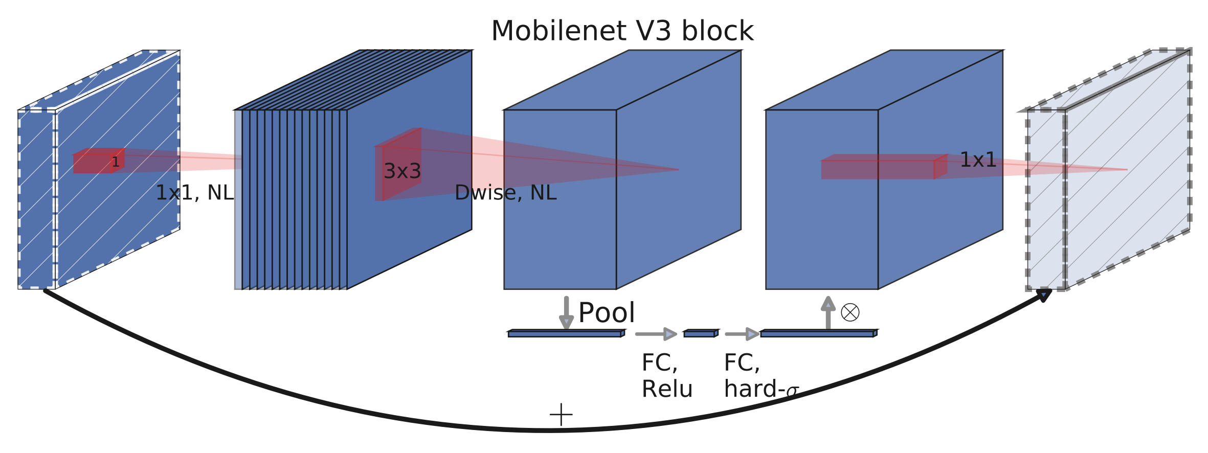
Olivier Cruchant is a Machine Learning Specialist Solutions Architect at AWS, based in Lyon, France. Olivier helps French customers – from small startups to large enterprises – develop and deploy production-grade machine learning applications. In his spare time, he enjoys reading research papers and exploring the wilderness with friends and family.

Read More

Host multiple TensorFlow computer vision models using Amazon SageMaker multi-model endpoints

Amazon SageMaker helps data scientists and developers prepare, build, train, and deploy high-quality machine learning (ML) models quickly by bringing together a broad set of capabilities purpose-built for ML. SageMaker accelerates innovation within your organization by providing purpose-built tools for every step of ML development, including labeling, data preparation, feature engineering, statistical bias detection, AutoML, training, tuning, hosting, explainability, monitoring, and workflow automation.

Companies are increasingly training ML models based on individual user data. For example, an image sharing service designed to enable discovery of information on the internet trains custom models based on each user’s uploaded images and browsing history to personalize recommendations for that user. The company can also train custom models based on search topics for recommending images per topic. Building custom ML models for each use case leads to higher inference accuracy, but increases the cost of deploying and managing models. These challenges become more pronounced when not all models are accessed at the same rate but still need to be available at all times.

SageMaker multi-model endpoints provide a scalable and cost-effective way to deploy large numbers of ML models in the cloud. SageMaker multi-model endpoints enable you to deploy multiple ML models behind a single endpoint and serve them using a single serving container. Your application simply needs to include an API call with the target model to this endpoint to achieve low-latency, high-throughput inference. Instead of paying for a separate endpoint for every single model, you can host many models for the price of a single endpoint. For more information about SageMaker multi-model endpoints, see Save on inference costs by using Amazon SageMaker multi-model endpoints.

In this post, we demonstrate how to use SageMaker multi-model endpoints to host two computer vision models with different model architectures and datasets for image classification. In practice, you can deploy tens of thousands of models on multi-model endpoints.

Overview of solution

SageMaker multi-model endpoints work with several frameworks, such as TensorFlow, PyTorch, MXNet, and sklearn, and you can build your own container with a multi-model server. Multi-model endpoints are also supported natively in the following popular SageMaker built-in algorithms: XGBoost, Linear Learner, Random Cut Forest (RCF), and K-Nearest Neighbors (KNN). You can directly use the SageMaker-provided containers while using these algorithms without having to build your own custom container.

The following diagram is a simplified illustration of how you can host multiple (for this post, six) models using SageMaker multi-model endpoints. In practice, multi-model endpoints can accommodate hundreds to tens of thousands of ML models behind an endpoint. In our architecture, if we host more models using model artifacts stored in Amazon Simple Storage Service (Amazon S3), multi-model endpoints dynamically unload some of the least-used models to accommodate newer models.

In this post, we show how to host two computer vision models trained using the TensorFlow framework behind a single SageMaker multi-model endpoint. We use the TensorFlow Serving container enabled for multi-model endpoints to host these models. For our first model, we train a smaller version of AlexNet CNN to classify images from the CIFAR-10 dataset. For the second model, we use a VGG16 CNN model pretrained on the ImageNet dataset and fine-tuned on the Sign Language Digits Dataset to classify hand symbol images. We also provide a fully functional notebook to demonstrate all the steps.

Model 1: CIFAR-10 image classification

CIFAR-10 is a benchmark dataset for image classification in computer vision and ML. CIFAR images are colored (three channels) with dramatic variation in how the objects appear. It consists of 32 × 32 color images in 10 classes, with 6,000 images per class. It contains 50,000 training images and 10,000 test images. The following image shows a sample of the images grouped by the labels.

To build the image classifier, we use a simplified version of the classical AlexNet CNN. The network is composed of five convolutional and pooling layers, and three fully connected layers. Our simplified architecture stacks three convolutional layers and two fully connected (dense) layers.

The first step is to load the dataset into train and test objects. The TensorFlow framework provides the CIFAR dataset for us to load using the load_data() method. Next, we rescale the input images by dividing the pixel values by 255: [0,255] ⇒ [0,1]. We also need to prepare the labels using one-hot encoding. One hot encoding is a process by which the categorical variables are converted into a numerical form. The following code snippet shows these steps in action:

from tensorflow.keras.datasets import cifar10

# load dataset
(X_train, y_train), (X_test, y_test) = cifar10.load_data()

# rescale input images
X_train = X_train.astype('float32')/255
X_test = X_test.astype('float32')/255

# one hot encode target labels
num_classes = len(np.unique(y_train))
y_train = utils.to_categorical(y_train, num_classes)
y_test = utils.to_categorical(y_test, num_classes)

After the dataset is prepared and ready for training, it’s saved to Amazon S3 to be used by SageMaker. The model architecture and the training code for the image classifier are assembled into a training script (cifar_train.py). To generate batches of tensor image data for the training process, we use ImageDataGenerator. This enables us to apply data augmentation transformations like rotation, width, and height shifts to our training data.

In the next step, we use the training script to create a TensorFlow estimator using the SageMaker SDK (see the following code). We use the estimator to fit the CNN model on CIFAR-10 inputs. When the training is complete, the model is saved to Amazon S3.

from sagemaker.tensorflow import TensorFlow

model_name = 'cifar-10'

hyperparameters = {'epochs': 50}

estimator_parameters = {'entry_point':'cifar_train.py',
                        'instance_type': 'ml.m5.2xlarge',
                        'instance_count': 2,
                        'model_dir': f'/opt/ml/model',
                        'role': role,
                        'hyperparameters': hyperparameters,
                        'output_path': f's3://{BUCKET}/{PREFIX}/cifar_10/out',
                        'base_job_name': f'mme-cv-{model_name}',
                        'framework_version': TF_FRAMEWORK_VERSION,
                        'py_version': 'py37',
                        'script_mode': True}

estimator_1 = TensorFlow(**estimator_parameters)

estimator_1.fit(inputs)

Later, we demonstrate how to host this model using SageMaker multi-model endpoint alongside our second model (the sign language digits classifier).

Model 2: Sign language digits classification

For our second model, we use the sign language digits dataset. This dataset distinguishes the sign language digits from 0–9. The following image shows a sample of the dataset.

The dataset contains 100 x 100 images in RGB color and has 10 classes (digits 0–9). The training set contains 1,712 images, the validation set 300, and the test set 50.

This dataset is very small. Training a network from scratch on this small a dataset doesn’t achieve good results. To achieve higher accuracy, we use transfer learning. Transfer learning is usually the go-to approach when starting a classification project, especially when you don’t have much training data. It migrates the knowledge learned from the source dataset to the target dataset, to save training time and computational cost.

To train this model, we use a pretrained VGG16 CNN model trained on the ImageNet dataset and fine-tune it to work on our sign language digits dataset. A pretrained model is a network that has been previously trained on a large dataset, typically on a large-scale image classification task. The VGG16 model architecture we use has 13 convolutional layers in total. For the sign language dataset, because its domain is different from the source domain of the ImageNet dataset, we only fine-tune the last few layers. Fine-tuning here refers to freezing a few of the network layers that are used for feature extraction, and jointly training both the non-frozen layers and the newly added classifier layers of the pretrained model.

The training script (sign_language_train.py) encapsulates the model architecture and the training logic for the sign language digits classifier. First, we load the pretrained weights from the VGG16 network trained on the ImageNet dataset. Next, we freeze part of the feature extractor part, followed by adding the new classifier layers. Finally, we compile the network and run the training process to optimize the model for the smaller dataset.

Next, we use this training script to create a TensorFlow estimator using the SageMaker SDK. This estimator is used to fit the sign language digits classifier on the supplied inputs. When the training is complete, the model is saved to Amazon S3 to be hosted by SageMaker multi-model endpoints. See the following code:

model_name = 'sign-language'

hyperparameters = {'epochs': 50}

estimator_parameters = {'entry_point':'sign_language_train.py',
                        'instance_type': 'ml.m5.2xlarge',
                        'instance_count': 2,
                        'hyperparameters': hyperparameters,
                        'model_dir': f'/opt/ml/model',
                        'role': role,
                        'output_path': f's3://{BUCKET}/{PREFIX}/sign_language/out',
                        'base_job_name': f'cv-{model_name}',
                        'framework_version': TF_FRAMEWORK_VERSION,
                        'py_version': 'py37',
                        'script_mode': True}

estimator_2 = TensorFlow(**estimator_parameters)

estimator_2.fit({'train': train_input, 'val': val_input})

Deploy a multi-model endpoint

SageMaker multi-model endpoints provide a scalable and cost-effective solution to deploy large numbers of models. It uses a shared serving container that is enabled to host multiple models. This reduces hosting costs by improving endpoint utilization compared to using single-model endpoints. It also reduces deployment overhead because SageMaker manages loading models in memory and scaling them based on the traffic patterns to them.

To create the multi-model endpoint, first we need to copy the trained models for the individual estimators (1 and 2) from their saved S3 locations to a common S3 prefix that can be used by the multi-model endpoint:

tf_model_1 = estimator_1.model_data
output_1 = f's3://{BUCKET}/{PREFIX}/mme/cifar.tar.gz'

tf_model_2 = estimator_2.model_data
output_2 = f's3://{BUCKET}/{PREFIX}/mme/sign-language.tar.gz'

!aws s3 cp {tf_model_1} {output_1}
!aws s3 cp {tf_model_2} {output_2}

After the models are copied to the common location designated by the S3 prefix, we create a serving model using the TensorFlowModel class from the SageMaker SDK. The serving model is created for one of the models to be hosted under the multi-model endpoint. In this case, we use the first model (the CIFAR-10 image classifier). Next, we use the MultiDataModel class from the SageMaker SDK to create a multi-model data model using the serving model for model-1, which we created in the previous step:

from sagemaker.tensorflow.serving import TensorFlowModel
from sagemaker.multidatamodel import MultiDataModel

model_1 = TensorFlowModel(model_data=output_1, 
                          role=role, 
                          image_uri=IMAGE_URI)

mme = MultiDataModel(name=f'mme-tensorflow-{current_time}',
                     model_data_prefix=model_data_prefix,
                     model=model_1,
                     sagemaker_session=sagemaker_session)

Finally, we deploy the MultiDataModel by calling the deploy() method, providing the attributes needed to create the hosting infrastructure required to back the multi-model endpoint:

predictor = mme.deploy(initial_instance_count=2,
                       instance_type='ml.m5.2xlarge',
                       endpoint_name=f'mme-tensorflow-{current_time}')

The deploy call returns a predictor instance, which we can use to make inference calls. We see this in the next section.

Test the multi-model endpoint for real-time inference

Multi-model endpoints enable sharing memory resources across your models. If the model to be referenced is already cached, multi-model endpoints run inference immediately. On the other hand, if the particular requested model isn’t cached, SageMaker has to download the model, which increases latency for that initial request. However, this takes only a fraction of the time it would take to launch an entirely new infrastructure (instances) to host the model individually on SageMaker. After a model is cached in the multi-model endpoint, subsequent requests are initiated in real time (unless the model is removed). As a result, you can run many models from a single instance, effectively decoupling our quantity of models from our cost of deployment. This makes it easy to manage ML deployments at scale and lowers your model deployment costs through increased usage of the endpoint and its underlying compute instances. For more information and a demonstration of cost savings of over 90% for a 1,000-model example, see Save on inference costs using Amazon SageMaker multi-model endpoints.

Multi-model endpoints also unload unused models from the container when the instances backing the endpoint reach memory capacity and more models need to be loaded into its container. SageMaker deletes unused model artifacts from the instance storage volume when the volume is reaching capacity and new models need to be downloaded. The first invocation to a newly added model takes longer because the endpoint takes time to download the model from Amazon S3 to the container’s memory of the instances backing the multi-model endpoint. Models that are unloaded remain on the instance’s storage volume and can be loaded into the container’s memory later without being downloaded again from the S3 bucket.

Let’s see how to make an inference from the CIFAR-10 image classifier (model-1) hosted under the multi-model endpoint. First, we load a sample image from one of the classes—airplane— and prepare it to be sent to the multi-model endpoint using the predictor we created in the previous step.

With this predictor, we can call the predict() method along with the initial_args parameter, which specifics the name of the target model to invoke. In this case, the target model is cifar.tar.gz. The following snippet demonstrates this process in detail:

img = load_img('./data/cifar_10/raw_images/airplane.png', target_size=(32, 32))
data = img_to_array(img)
data = data.astype('float32')
data = data / 255.0
data = data.reshape(1, 32, 32, 3)
payload = {'instances': data}
y_pred = predictor.predict(data=payload, initial_args={'TargetModel': 'cifar.tar.gz'})
predicted_label = CIFAR10_LABELS[np.argmax(y_pred)]
print(f'Predicted Label: [{predicted_label}]')

Running the preceding code returns the prediction output as the label airplane, which is correctly interpreted by our served model:

Predicted Label: [airplane]

Next, let’s see how to dynamically load the sign language digit classifier (model-2) into a multi-model endpoint by invoking the endpoint with sign-language.tar.gz as the target model.

We use the following sample image of the hand sign digit 0.

The following snippet shows how to invoke the multi-model endpoint with the sample image to get back the correct response:

test_path  = './data/sign_language/test'
img = mpimg.imread(f'{test_path}/0/IMG_4159.JPG')

def path_to_tensor(img_path):
    # loads RGB image as PIL.Image.Image type
    img = image.load_img(img_path, target_size=(224, 224))
    # convert PIL.Image.Image type to 3D tensor with shape (224, 224, 3)
    x = image.img_to_array(img)
    # convert 3D tensor to 4D tensor with shape (1, 224, 224, 3) and return 4D tensor
    return np.expand_dims(x, axis=0)

data = path_to_tensor(f'{test_path}/0/IMG_4159.JPG')
payload = {'instances': data}
y_pred = predictor.predict(data=payload, initial_args={'TargetModel': 'sign-language.tar.gz'})predicted_label = np.argmax(y_pred)
print(f'Predicted Label: [{predicted_label}]')

The following code is our response, with the label 0:

Predicted Label: [0]

Conclusion

In this post, we demonstrated the SageMaker feature multi-model endpoints to optimize inference costs. Multi-model endpoints are useful when you’re dealing with hundreds to tens of thousands of models and where you don’t need to deploy each model as an individual endpoint. Models are loaded and unloaded dynamically, according to usage and the amount of memory available on the endpoint.

This post discussed how to host multiple computer vision models trained using the TensorFlow framework under one SageMaker multi-model endpoint. The image classification models were of different model architectures and trained on different datasets. The notebook included with the post provides detailed instructions on training and hosting the models.

Give SageMaker multi-model endpoints a try for your use case and leave your feedback in the comments.


About the Authors

Arunprasath Shankar is an Artificial Intelligence and Machine Learning (AI/ML) Specialist Solutions Architect with AWS, helping global customers scale their AI solutions effectively and efficiently in the cloud. In his spare time, Arun enjoys watching sci-fi movies and listening to classical music.


Mark Roy is a Principal Machine Learning Architect for AWS, helping AWS customers design and build AI/ML solutions. Mark’s work covers a wide range of ML use cases, with a primary interest in computer vision, deep learning, and scaling ML across the enterprise. He has helped companies in many industries, including Insurance, Financial Services, Media and Entertainment, Healthcare, Utilities, and Manufacturing. Mark holds six AWS certifications, including the ML Specialty Certification. Prior to joining AWS, Mark was an architect, developer, and technology leader for 25+ years, including 19 years in financial services.

Read More