In this work, we use deep reinforcement learning to generate artificial agents capable of test-time cultural transmission. Once trained, our agents can infer and recall navigational knowledge demonstrated by experts. This knowledge transfer happens in real time and generalises across a vast space of previously unseen tasks.Read More
Beyond Be-leaf: Immersive 3D Experience Transports Audiences to Natural Worlds With Augmented Reality
Imagine walking through the bustling streets of London’s Piccadilly Circus, when suddenly you’re in a tropical rainforest, surrounded by vibrant flowers and dancing butterflies.
That’s what audiences will see in the virtual world of The Green Planet AR Experience, an interactive, augmented reality experience that blends physical and digital worlds to connect people with nature.
During the Green Planet AR Experience, powered by EE 5G, visitors are led through a living rainforest and six distinct biomes by a 3D hologram of Sir David Attenborough, familiar to many as the narrator of some of the world’s most-watched nature documentaries.

Audiences engage and interact with the plant life by using a mobile device, which acts as a window into the natural world.
To bring these virtual worlds to life in a sustainable way, award-winning studio Factory 42 combined captivating storytelling with cutting-edge technology. Using NVIDIA RTX and CloudXR, the creative team elevated the AR experience and delivered high-fidelity, photorealistic virtual environments over a 5G network.
Natural, Immersive AR Over 5G — It’s a Stream Come True
The Green Planet AR Experience’s mission is to inspire, educate and motivate visitors toward positive change by showcasing how plants are vital to all life on earth. Through the project, Factory 42 and the BBC help audiences gain a deeper understanding of ecosystems, the importance of biodiversity and what it means to protect our planet.
To create an immersive environment that captured the rich, vivid colors and details of natural worlds, the Factory 42 team needed high-quality imagery and graphics power. Using mobile edge computing allowed them to deliver the interactive experience to a large number of users over EE’s private 5G network.
The AR experience runs on a custom, on-premises GPU edge-rendering stack powered by NVIDIA RTX 8000 professional GPUs. Using NVIDIA RTX, Factory 42 created ultra-high-quality 3D digital assets, environments, interactions and visual effects that made the natural elements look as realistic as possible.

With the help of U.K.-based integrator The GRID Factory, the GPU edge-rendering stack is connected to EE’s private 5G network using the latest Ericsson Industry Connect solution for a dedicated wireless cellular network. Using NVIDIA RTX Virtual Workstation (RTX vWS) on VMware Horizon, and NVIDIA’s advanced CloudXR streaming solution, Factory 42 can stream all the content from the edge of the private 5G network to the Samsung S21 mobile handsets used by each visitor.
“NVIDIA RTX vWS and CloudXR were a step ahead of the competitive products — their robustness, ability to fractionalize the GPU, and high-quality delivery of streamed XR content were key features that allowed us to create our Green Planet AR Experience as a group experience to thousands of users,” said Stephen Stewart, CTO at Factory 42.
The creative team at Factory 42 designed the content in the AR environment, which is rendered in real time with the Unity game engine. The 3D hologram of Sir David was created using volumetric capture technology provided by Dimension Studios. Spatial audio provides a surround-sound setup, which guides people through the virtual environment as digital plants and animals react to the presence of visitors in the space.
Combining these technologies, Factory42 created a new level of immersive experience — one only made possible through 5G networks.
“NVIDIA RTX and CloudXR are fundamental to our ability to deliver this 5G mobile edge compute experience,” said Stewart. “The RTX 8000 GPU provided the graphics power and the NVENC support required to deploy into an edge rendering cluster. And with CloudXR, we could create robust connections to mobile handsets.”

Sustainability was considered at every level of construction and operation. The materials used in building The Green Planet AR Experience will be reused or recycled after the event to promote circularity. And combining NVIDIA RTX and CloudXR with 5G, Factory 42 can give audiences interactive experiences with hundreds of different trees, plants and creatures inside an eco-friendly, virtual space.
Experience the Future of Streaming at GTC
Learn more about how NVIDIA is helping companies create unforgettable immersive experiences at GTC, which runs from March 21-24.
Registration is free. Sign up to hear from leading companies and professionals across industries, including Factory 42, as they share insights about the future of AR, VR and other extended reality applications.
And watch the keynote address by NVIDIA CEO Jensen Huang, on March 22 at 8 a.m. Pacific, to hear the latest news on NVIDIA technologies.
The post Beyond Be-leaf: Immersive 3D Experience Transports Audiences to Natural Worlds With Augmented Reality appeared first on NVIDIA Blog.

Using Deep Learning to Annotate the Protein Universe
Proteins are essential molecules found in all living things. They play a central role in our bodies’ structure and function, and they are also featured in many products that we encounter every day, from medications to household items like laundry detergent. Each protein is a chain of amino acid building blocks, and just as an image may include multiple objects, like a dog and a cat, a protein may also have multiple components, which are called protein domains. Understanding the relationship between a protein’s amino acid sequence — for example, its domains — and its structure or function are long-standing challenges with far-reaching scientific implications.
| An example of a protein with known structure, TrpCF from E. coli, for which areas used by a model to predict function are highlighted (green). This protein produces tryptophan, which is an essential part of a person’s diet. |
<!–
 |
| An example of a protein with known structure, TrpCF from E. coli, for which areas used by a model to predict function are highlighted (green). This protein produces tryptophan, which is an essential part of a person’s diet. |
–>
Many are familiar with recent advances in computationally predicting protein structure from amino acid sequences, as seen with DeepMind’s AlphaFold. Similarly, the scientific community has a long history of using computational tools to infer protein function directly from sequences. For example, the widely-used protein family database Pfam contains numerous highly-detailed computational annotations that describe a protein domain’s function, e.g., the globin and trypsin families. While existing approaches have been successful at predicting the function of hundreds of millions of proteins, there are still many more with unknown functions — for example, at least one-third of microbial proteins are not reliably annotated. As the volume and diversity of protein sequences in public databases continue to increase rapidly, the challenge of accurately predicting function for highly divergent sequences becomes increasingly pressing.
In “Using Deep Learning to Annotate the Protein Universe”, published in Nature Biotechnology, we describe a machine learning (ML) technique to reliably predict the function of proteins. This approach, which we call ProtENN, has enabled us to add about 6.8 million entries to Pfam’s well-known and trusted set of protein function annotations, about equivalent to the sum of progress over the last decade, which we are releasing as Pfam-N. To encourage further research in this direction, we are releasing the ProtENN model and a distill-like interactive article where researchers can experiment with our techniques. This interactive tool allows the user to enter a sequence and get results for a predicted protein function in real time, in the browser, with no setup required. In this post, we’ll give an overview of this achievement and how we’re making progress toward revealing more of the protein universe.
 |
| The Pfam database is a large collection of protein families and their sequences. Our ML model ProtENN helped annotate 6.8 million more protein regions in the database. |
Protein Function Prediction as a Classification Problem
In computer vision, it’s common to first train a model for image classification tasks, like CIFAR-100, before extending it to more specialized tasks, like object detection and localization. Similarly, we develop a protein domain classification model as a first step towards future models for classification of entire protein sequences. We frame the problem as a multi-class classification task in which we predict a single label out of 17,929 classes — all classes contained in the Pfam database — given a protein domain’s sequence of amino acids.
Models that Link Sequence to Function
While there are a number of models currently available for protein domain classification, one drawback of the current state-of-the-art methods is that they are based on the alignment of linear sequences and don’t consider interactions between amino acids in different parts of protein sequences. But proteins don’t just stay as a line of amino acids, they fold in on themselves such that nonadjacent amino acids have strong effects on each other.
Aligning a new query sequence to one or more sequences with known function is a key step of current state-of-the-art methods. This reliance on sequences with known function makes it challenging to predict a new sequence’s function if it is highly dissimilar to any sequence with known function. Furthermore, alignment-based methods are computationally intensive, and applying them to large datasets, such as the metagenomic database MGnify, which contains >1 billion protein sequences, can be cost prohibitive.
To address these challenges, we propose to use dilated convolutional neural networks (CNNs), which should be well-suited to modeling non-local pairwise amino-acid interactions and can be run on modern ML hardware like GPUs. We train 1-dimensional CNNs to predict the classification of protein sequences, which we call ProtCNN, as well as an ensemble of independently trained ProtCNN models, which we call ProtENN. Our goal for using this approach is to add knowledge to the scientific literature by developing a reliable ML approach that complements traditional alignment-based methods. To demonstrate this, we developed a method to accurately measure our method’s accuracy.
Evaluation with Evolution in Mind
Similar to well-known classification problems in other fields, the challenge in protein function prediction is less in developing a completely new model for the task, and more in creating fair training and test sets to ensure that the models will make accurate predictions for unseen data. Because proteins have evolved from shared common ancestors, different proteins often share a substantial fraction of their amino acid sequence. Without proper care, the test set could be dominated by samples that are highly similar to the training data, which could lead to the models performing well by simply “memorizing” the training data, rather than learning to generalize more broadly from it.
| We create a test set that requires ProtENN to generalize well on data far from its training set. |
<!–
 |
| We create a test set that requires ProtENN to generalize well on data far from its training set. |
–>
To guard against this, it is essential to evaluate model performance using multiple separate setups. For each evaluation, we stratify model accuracy as a function of similarity between each held-out test sequence and the nearest sequence in the train set.
The first evaluation includes a clustered split training and test set, consistent with prior literature. Here, protein sequence samples are clustered by sequence similarity, and entire clusters are placed into either the train or test sets. As a result, every test example is at least 75% different from every training example. Strong performance on this task demonstrates that a model can generalize to make accurate predictions for out-of-distribution data.
For the second evaluation, we use a randomly split training and test set, where we stratify examples based on an estimate of how difficult they will be to classify. These measures of difficulty include: (1) the similarity between a test example and the nearest training example, and (2) the number of training examples from the true class (it is much more difficult to accurately predict function given just a handful of training examples).
To place our work in context, we evaluate the performance of the most widely used baseline models and evaluation setups, with the following baseline models in particular: (1) BLAST, a nearest-neighbor method that uses sequence alignment to measure distance and infer function, and (2) profile hidden Markov models (TPHMM and phmmer). For each of these, we include the stratification of model performance based on sequence alignment similarity mentioned above. We compared these baselines against ProtCNN and the ensemble of CNNs, ProtENN.
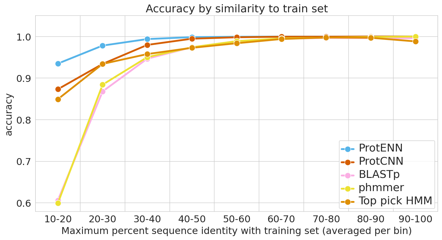 |
| We measure each model’s ability to generalize, from the hardest examples (left) to the easiest (right). |
Reproducible and Interpretable Results
We also worked with the Pfam team to test whether our methodological proof of concept could be used to label real-world sequences. We demonstrated that ProtENN learns complementary information to alignment-based methods, and created an ensemble of the two approaches to label more sequences than either method could by itself. We publicly released the results of this effort, Pfam-N, a set of 6.8 million new protein sequence annotations.
After seeing the success of these methods and classification tasks, we inspected these networks to understand whether the embeddings were generally useful. We built a tool that enables users to explore the relation between the model predictions, embeddings, and input sequences, which we have made available through our interactive manuscript, and we found that similar sequences were clustered together in embedding space. Furthermore, the network architecture that we selected, a dilated CNN, allows us to employ previously-discovered interpretability methods like class activation mapping (CAM) and sufficient input subsets (SIS) to identify the sub-sequences responsible for the neural network predictions. With this approach, we find that our network generally focuses on the relevant elements of a sequence to predict its function.
Conclusion and Future Work
We’re excited about the progress we’ve seen by applying ML to the understanding of protein structure and function over the last few years, which has been reflected in contributions from the broader research community, from AlphaFold and CAFA to the multitude of workshops and research presentations devoted to this topic at conferences. As we look to build on this work, we think that continuing to collaborate with scientists across the field who’ve shared their expertise and data, combined with advances in ML will help us further reveal the protein universe.
Acknowledgments
We’d like to thank all of the co-authors of the manuscripts, Maysam Moussalem, Jamie Smith, Eli Bixby, Babak Alipanahi, Shanqing Cai, Cory McLean, Abhinay Ramparasad, Steven Kearnes, Zack Nado, and Tom Small.

Machine learning can help read the language of life
DNA is the language of life: our DNA forms a living record of things that went well for our ancestors, and things that didn’t. DNA tells our body (and every other organism) which proteins to produce; these proteins are tiny machines that carry out enormous tasks, from fighting off infection to helping you ace an upcoming exam in school.
But for about a third of all proteins that all organisms produce, we just don’t know what they do. It’s kind of like we’re in a factory where everything’s buzzing, and we’re surrounded by all these impressive tools, but we have only a vague idea of what’s going on. Understanding how these tools operate, and how we can use them, is where we think machine learning can make a big difference.
An example of a previously-solved protein structure (E. coli TrpCF) and the area where our AI makes predictions of its function. This protein produces tryptophan, which is a chemical that’s required in your diet to keep your body and brain running.
Recently, DeepMind showed that AlphaFold can predict the shape of protein machinery with unprecedented accuracy. The shape of a protein provides very strong clues as to how the protein machinery can be used, but doesn’t completely solve this question. So we asked ourselves: can we predict what function a protein performs?
In our Nature Biotechnology article, we describe how neural networks can reliably reveal the function of this “dark matter” of the protein universe, outperforming state-of-the-art methods. We worked closely with internationally recognized experts at the European Bioinformatics Institute to annotate 6.8 million more protein regions in the Pfam v34.0 database release, a global repository for protein families and their function. These annotations exceed the expansion of the database over the last decade, and will enable the 2.5 million life-science researchers around the world to discover new antibodies, enzymes, foods, and therapeutics.
The Pfam database is a large collection of protein families and their sequences. Our ML models helped annotate 6.8 million more protein regions in the database.
We also understand there’s a reproducibility crisis in science, and we want to be part of the solution — not the problem. To make our research more accessible and useful, we’re excited to launch an interactive scientific article where you can play with our ML models — getting results in real time, all in your web browser, with no setup required.
Google has always set out to help organize the world’s information, and to make it useful to everyone. Equity in access to the appropriate technology and useful instruction for all scientists is an important part of this mission. This is why we’re committed to making these models useful and accessible. Because, who knows, one of these proteins could unlock the solution to antibiotic resistance, and it’s sitting right under our noses.
A new resource for teaching responsible technology development
Understanding the broader societal context of technology is becoming ever more critical as advances in computing show no signs of slowing. As students code, experiment, and build systems, being able to ask questions and make sense of hard problems involving social and ethical responsibility is as important as the technology they’re studying and developing.
To train students to practice responsible technology development and provide opportunities to have these conversations in the classroom setting, members from across computing, data sciences, humanities, arts, and social sciences have been collaborating to craft original pedagogical materials that can be incorporated into existing classes at MIT.
All of the materials, created through the Social and Ethical Responsibilities of Computing (SERC), a cross-cutting initiative of the MIT Schwarzman College of Computing, are now freely available via MIT OpenCourseWare (OCW). The collection includes original active learning projects, homework assignments, in-class demonstrations, and other resources and tools found useful in education at MIT.
“We’re delighted to partner with OCW to make these materials widely available. By doing so, our goal is to enable instructors to incorporate them into their courses so that students can gain hands-on practice and training in SERC,” says Julie Shah, associate dean of SERC and professor of aeronautics and astronautics.
For the last two years, SERC has been bringing together cross-disciplinary teams of faculty, researchers, and students to generate the original content. Most of the materials featured on OCW were produced by participants in SERC’s semester-long Action Groups on Active Learning Projects in which faculty from humanities, arts, and social sciences are paired with faculty in computing and data sciences to collaborate on new projects for each of their existing courses. Throughout the semester, the action groups worked with SERC on content development and pilot-tested the new materials before the results were published.
The associated instructors who created course materials featured on the new resource site include Leslie Kaelbling for class 6.036 (Introduction to Machine Learning), Daniel Jackson and Arvind Satyanaran for class 6.170 (Software Studio), Jacob Andreas and Catherine D’Ignazio for class 6.864 (Natural Language Processing), Dwai Banerjee for STS.012 (Science in Action: Technologies and Controversies in Everyday Life), and Will Deringer for STS.047 (Quantifying People: A History of Social Science). SERC also enlisted a number of graduate students and postdocs to help the instructors develop the materials.
Andreas, D’Ignazio, and PhD student Harini Suresh recently reflected on their effort together in an episode of Chalk Radio, the OCW podcast about inspired teaching at MIT. Andreas observed that students at MIT and elsewhere take classes in advanced computing techniques like machine learning, but there is still often a “gap between the way we are training these people and the way these tools are getting deployed in practice.” “The thing that surprised me most,” he continued, “was the number of students who said, ‘I’ve never done an assignment like this in my whole undergraduate or graduate training.’”
In a second SERC podcast episode, released on Feb. 23, computer science professor Jackson and graduate student Serena Booth discuss ethics, software design, and impact on everyday people.
Organized by topic areas, including privacy and surveillance; inequality, justice, and human rights; artificial intelligence and algorithms; social and environmental impacts; autonomous systems and robotics; ethical computing and practice; and law and policy, the site also spotlights materials from the MIT Case Studies in Social and Ethical Responsibilities of Computing, an ongoing series that examines social, ethical, and policy challenges of present-day efforts in computing. The specially commissioned and peer-reviewed case studies are brief and intended to be effective for undergraduate instruction across a range of classes and fields of study. Like the new materials on MIT OpenCourseWare, the SERC Case Studies series is made available for free via open-access publishing.
Several issues have been published to date since the series launched in February 2020. The latest issue, the third in the series which was released just last month, comprises five original case studies that explore a range of subjects from whether the rise of automation is a threat to the American workforce to the role algorithms play in electoral redistricting. Penned by faculty and researchers from across MIT as well as from Vanderbilt University and George Washington University, all of the cases are based on the authors’ original research.
With many more in the pipeline, new content will be published on OCW twice a year to keep the site updated with SERC-related materials.
“With computing being one of OCW’s most popular topics, this spotlight on social and ethical responsibility will reach millions of learners,” says Curt Newton, director of OCW. “And by sharing how MIT faculty and students use the materials, we’re creating pathways for educators around the world to adapt the materials for maximum relevance to their students.”
Amazon VP Babak Parviz appointed to AAAS Board of Directors
Parviz will serve a three-year term as one of four appointed directors.Read More
Bundesliga Match Fact Set Piece Threat: Evaluating team performance in set pieces on AWS
The importance of set pieces in football (or soccer in the US) has been on the rise in recent years: now more than one quarter of all goals are scored via set pieces. Free kicks and corners generally create the most promising situations, and some professional teams have even hired specific coaches for those parts of the game.
In this post, we share how the Bundesliga Match Fact Set Piece Threat helps evaluate performance in set pieces. As teams look to capitalize more and more on these dead ball situations, Set Piece Threat will help the viewer understand how well teams are leveraging these situations. In addition, it will explain the reader how AWS services can be used to compute statistics in real-time.
Bundesliga’s Union Berlin is a great example for the relevance of set pieces. The team managed to rise from Bundesliga 2 to qualification for a European competition in just 2 years. They finished third in Bundesliga 2 during the 18/19 season, earning themselves a slot in the relegation playoffs to the Bundesliga. In that season, they scored 28 goals from open play, ranking just ninth in the league. However, they ranked second for goals scored through set pieces (16 goals).
Tellingly, in the first relegation playoff match against VfB Stuttgart, Union secured a 2:2 draw, scoring a header after a corner. And in the return match, Stuttgart was disallowed a free kick goal due to a passive offside, allowing Union to enter the Bundesliga with a 0:0 draw.
The relevance of set pieces for Union’s success doesn’t end there. Union finished their first two Bundesliga seasons with strong eleventh and seventh, ranking third and first in number of set piece goals (scoring 15 goals from set pieces in both seasons). For comparison, FC Bayern München—the league champion—only managed to score 10 goals from set pieces in both seasons. The success that Union Berlin has had with their set pieces allowed them to secure the seventh place in the 20/21 Bundesliga season, which meant qualification for the UEFA Europa Conference League, going from Bundesliga 2 to Europe just 2 years after having earned promotion. Unsurprisingly, in the deciding match, they scored one of their two goals after a corner. At the time of this writing, Union Berlin ranks fourth in the Bundesliga (matchday 20) and first in corner performance, a statistic we explain later.
Union Berlin’s path to Europe clearly demonstrates the influential role of offensive and defensive performance during set pieces. Until now however, it was difficult for fans and broadcasters to properly quantify this performance, unless they wanted to dissect massive tables on analytics websites. Bundesliga and AWS have worked together to illustrate the threat that a team produces and the threat that is produced by set pieces against the team, and came up with the new Bundesliga Match Fact: Set Piece Threat.
How does Set Piece Threat work?
To determine the threat a team poses with their set pieces, we take into account different facets of their set piece performance. It’s important to note that we only consider corners and free kicks as set pieces, and compute the threat for each category independently.
Facet 1: Outcome of a set piece: Goals, shots, or nothing
First, we consider the outcome of a set piece. That is, we observe if it results in a goal. However, the outcome is generally influenced by fine margins, such as a great save by the goal keeper or if a shot brushes the post instead of going in, so we also categorize the quality of a shot that results from the set piece. Shots are categorized into several categories.
| Category | Explanation |
| Goal | A successful shot that lead to a goal |
| Outstanding | Shots that almost led to a goal, such as a shot at the post |
| Decent | Other noteworthy goals scenes |
| Average | The rest of the chances that would be included in a chances ratio with relevant threat of a goal |
| None | No real goal threat, should not be considered a real chance, such as a header that barely touched the ball or a blocked shot |
| No shot | No shots taken at all |
The above video shows examples of shot outcome categories in the following order: outstanding, decent, average, none.
Facet 2: Potential of a shot
Second, our algorithm considers the potential of a shot. This incorporates how likely it should have resulted in a goal, taking the actual performance of the shot-taker out of the equation. In other words, we quantify the goal potential of the situation in which the shot was taken. This is captured by the expected goal (xGoals) value of the shot. We remove not only the occurrence of luck or lack thereof, but also the quality of the strike or header.

Facet 3: Quantity of set pieces
Next, we consider the aspect of pure quantity of set pieces that a team gets. Our definition of Set Piece Threat measures the threat on a per-set-piece-basis. Instead of summing up all outcomes and xGoal values of a team over the course of a season, the values are aggregated such that they represent the average threat per set piece. That way, the corner threat, for example, represents the team’s danger for each corner and doesn’t consider a team more dangerous simply because they have more corners than other teams (and therefore potentially more shots or goals).
Facet 4: Development over time
The last aspect to consider is the development of a team’s threat over time. Consider for example a team that scored three goals from corners in the first three matchdays but fails to deliver any considerable threat over the next 15 matchdays. This team should not be considered to pose a significant threat from corners on matchday 19, despite it already having scored three times, which may still be a good return. We account for this (positive or negative) development of a team’s set piece quality by assigning a discount to each set piece, depending on how long ago it occurred. In other words, a free kick that was taken 10 matchdays ago has less influence on the computed threat than one that was taken during the last or even current game.
Score: Per set piece aggregation
All four facets we’ve described are aggregated into two values for each team, one for corners and one for free kicks, which describe the danger that a corresponding set piece by that team would currently pose. The value is defined as the weighted average of the scores of each set piece, where the score of a set piece is defined as (0.7 * shot-outcome + 0.3 * xG-value) if the set piece resulted in a shot and 0 otherwise. The shot-outcome is 1 if the team scored and lower for other outcomes, such as a shot that went wide, depending on its quality. The weight for each set piece is determined by how long ago it was taken, as described earlier. Overall, the values are defined between 0–1, where 1 is the perfect score.

Set piece threat
Next, the values for each team are compared to the league average. The exact formula is score(team)/avg_score(league) - 1. This value is what we call the Set Piece Threat value. A team has a threat value of 0 if it’s exactly as good as the league average. A value of -1 (or -100%) describes a team that poses no threat at all, and a value of +1 (+100%) describes a team that is twice as dangerous as the league average. With those values, we compute a ranking that orders the teams from 1–18 according to their offensive threat of corners and free kicks, respectively.
 |
 |
We use the same data and similar calculations to also compute a defensive threat that measures the defensive performance of a team with regard to how they defend set pieces. Now, instead of computing a score per own set piece, the algorithm computes a score per opponent set piece. Just like for the offensive threat, the score is compared to the league average, but the value is reversed: -score(team)/avg_score(league) + 1. This way, a threat of +1 (+100%) is achieved if team allows opponents no shots at all, whereas a team with defensive threat of -1 (-100%) is twice as susceptible to opponents’ set pieces as the league average. Again, a team with a threat of 0 is as good as the league average.


Set Piece Threat findings
An important aspect of Set Piece Threat is that we focus on an estimation of threat instead of goals scored and conceded via set pieces. If we take SC Freiburg and Union Berlin at matchday 21 as an example, over the course of this season Freiburg has scored seven goals via corners in comparison to four from Union Berlin. Our threat ranking still ranks both of the teams fairly equal. In fact, we predict a corner by Freiburg (Rank 3) to even be 7% less threatening than a corner by Union Berlin (Rank 1). The main reason for this is that Union Berlin created a similar number of great chances out of their corners, but failed to convert these chances into goals. Freiburg on the other hand was vastly more efficient with their chances. Such a discrepancy between chance quality and actual goals can happen in a high-variance sport like football.
The following graph shows Union Berlin’s set piece offensive corner ranking (blue) and score (red) from matchdays 6–21. At matchday 12, Union scored a goal from a corner and additionally had a great chance from a second corner that didn’t result in a goal but was perceived as a high threat by our algorithm. In addition, Union had a shot on target in five of seven corner kicks on matchday 12. Union immediately jumped in the ranking from twelfth to fifth place as a result of this, and the score value for Union increased as well as the league average. As Union saw more and more high threat chances in the later matchdays from corners, they step by step claimed first place of the corner threat ranking. The score is always relative to the current league average, meaning that Union’s threat at matchday 21 is 50% higher from corners than the average threat coming from all teams in the league.

Implementation and architecture
Bundesliga Match Facts are independently running AWS Fargate containers inside Amazon Elastic Container Service (Amazon ECS). Previous Bundesliga Match Facts consume raw event and positional data to calculate advanced statistics. This changes with the release of Set Piece Threat, which analyzes data produced by an existing Bundesliga Match Fact (xGoals) to calculate its rankings. Therefore, we created an architecture to exchange messages between different Bundesliga Match Facts during live matches in real time.
To guarantee the latest data is reflected in the set piece threat calculations, we use Amazon Managed Streaming for Apache Kafka (Amazon MSK). This message broker service allows different Bundesliga Match Facts to send and receive the newest events and updates in real time. By consuming a match and Bundesliga Match Fact-specific topic from Kafka, we can receive the most up-to-date data from all systems involved while retaining the ability to replay and reprocess messages sent earlier.
The following diagram illustrates the solution architecture:

We introduced Amazon MSK to this project to generally replace all internal message passing for the Bundesliga Match Facts platform. It handles the injection of positional and event data, which can aggregate to over 3.6 million data points per match. With Amazon MSK, we can use the underlying persistent storage of messages, which allows us to replay games from any point in time. However, for Set Piece Threat, the focus lies on the specific use case of passing events produced by Bundesliga Match Facts to other Bundesliga Match Facts that are running in parallel.
To facilitate this, we distinguish between two types of Kafka topics: global and match-specific. First, each Bundesliga Match Fact has an own specific global topic, which handles all messages created by the Bundesliga Match Fact. Additionally, there is an additional match-specific topic for each Bundesliga Match Fact for each match that is handling all messages created by a Bundesliga Match Fact for a specific match. When multiple live matches run in parallel, each message is first produced and sent to this Bundesliga Match Fact-specific global topic.
A dispatcher AWS Lambda function is subscribed to every Bundesliga Match Fact-specific global topic and has two tasks:
- Write the incoming data to a database provisioned through Amazon Relational Database Service (Amazon RDS).
- Redistribute the messages that can be consumed by other Bundesliga Match Facts to a Bundesliga Match Fact-specific topic.
The left side of the architecture diagram shows the different Bundesliga Match Facts running independently from each other for every match and producing messages to the global topic. The new Set Piece Threat Bundesliga Match Fact now can consume the latest xGoal values for each shot for a specific match (right side of the diagram) to immediately compute the threat produced by the set piece that resulted in one or more shots.
Summary
We’re excited about the launch of Set Piece Threat and the patterns commentators and fans will uncover using this brand-new insight. As teams look to capitalize more and more on these dead ball situations, Set Piece Threat will help the viewer understand which team is doing this successfully and which team still has some ground to cover, which adds additional suspense before each of these set piece situations. The new Bundesliga Match Fact is available to Bundesliga’s broadcasters to uncover new perspectives and stories of a match, and team rankings can be viewed at any time in the Bundesliga app.
We’re excited to learn what patterns you will uncover. Share your insights with us: @AWScloud on Twitter, with the hashtag #BundesligaMatchFacts.
About the Authors
Simon Rolfes played 288 Bundesliga games as a central midfielder, scored 41 goals and won 26 caps for Germany. Currently Rolfes serves as Sporting Director at Bayer 04 Leverkusen where he oversees and develops the pro player roster, the scouting department and the club’s youth development. Simon also writes weekly columns on Bundesliga.com about the latest Bundesliga Match Facts powered by AWS
Luuk Figdor is a Senior Sports Technology Specialist in the AWS Professional Services team. He works with players, clubs, leagues, and media companies such as Bundesliga and Formula 1 to help them tell stories with data using machine learning. In his spare time, he likes to learn all about the mind and the intersection between psychology, economics, and AI.
Jan Bauer is a Cloud Application Architect at AWS Professional Services. His interests are serverless computing, machine learning, and everything that involves cloud computing. He works with clients across industries to help them be successful on their cloud journey.
Pascal Kühner is a Cloud Application Developer in the AWS Professional Services Team. He works with customers across industries to help them achieve their business outcomes via application development, DevOps, and infrastructure. He loves ball sports and in his spare time likes to play basketball and football.
Uwe Dick is a Data Scientist at Sportec Solutions AG. He works to enable Bundesliga clubs and media to optimize their performance using advanced stats and data—before, after, and during matches. In his spare time, he settles for less and just tries to last the full 90 minutes for his recreational football team.
Javier Poveda-Panter is a Data Scientist for EMEA sports customers within the AWS Professional Services team. He enables customers in the area of spectator sports to innovate and capitalize on their data, delivering high quality user and fan experiences through machine learning and data science. He follows his passion for a broad range of sports, music and AI in his spare time.
Bundesliga Match Fact Skill: Quantifying football player qualities using machine learning on AWS
In football, as in many sports, discussions about individual players have always been part of the fun. “Who is the best scorer?” or “Who is the king of defenders?” are questions perennially debated by fans, and social media amplifies this debate. Just consider that Erling Haaland, Robert Lewandowski, and Thomas Müller alone have a combined 50 million followers on Instagram. Many fans are aware of the incredible statistics star players like Lewandowski and Haaland create, but stories like this are just the tip of the iceberg.
Consider that almost 600 players are under contract in the Bundesliga, and each team has their own champions—players that get introduced to bring a specific skill to bear in a match. Look for example at Michael Gregoritsch of FC Augsburg. As of this writing (matchday 21), he has scored five goals in the 21/22 season, not something that would make anybody mention him in a conversation about the great goal scorers. But let’s look closer: if you accumulate the expected goal (xGoals) values of all scoring chances Gregoritsch had this season, the figure you get is 1.7. This means he over-performed on his shots on goal by +194%, scoring 3.2 more goals than expected. In comparison, Lewandowski over-performed by only 1.6 goals (+7%). What a feat! Clearly Gregoritsch brings a special skill to Augsburg.
So how do we shed light on all the hidden stories about individual Bundesliga players, their skills, and impact on match outcomes? Enter the new Bundesliga Match Fact powered by AWS called Skill. Skill has been developed through in-depth analysis by the DFL and AWS to identify players with skills in four specific categories: initiator, finisher, ball winner, and sprinter. This post provides a deep dive into these four skills and discusses how they are implemented on AWS infrastructure.
Another interesting point is that until now, Bundesliga Match Facts have been developed independent from one another. Skill is the first Bundesliga Match Fact that combines the output of multiple Bundesliga Match Facts in real time using a streaming architecture built on Amazon Managed Streaming Kafka (Amazon MSK).
Initiator
An initiator is a player who performs a high number of valuable first and second assists. To identify and quantify the value of those assists, we introduced the new metric xAssist. It’s calculated by tracking the last and second-last pass before a shot at goal, and assigning the respective xGoals value to those actions. A good initiator creates opportunities under challenging circumstances by successfully completing passes with a rate of high difficulty. To evaluate how hard it is to complete a given pass, we use our existing xPass model. In this metric, we purposely exclude crosses and free kicks to focus on players who generate scoring chances with their precise assists from open play.
The skill score is calculated with the following formula:

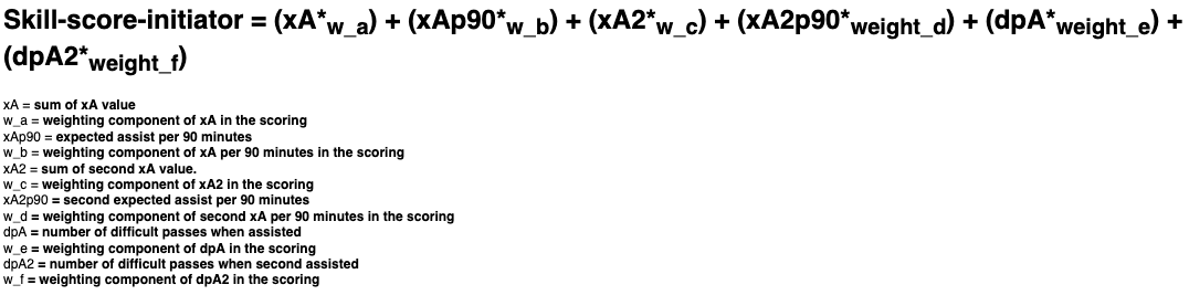
Let’s look at the current Rank 1 initiator, Thomas Müller, as an example. He has collected an xAssist value of 9.23 as of this writing (matchday 21), meaning that his passes for the next players who shot at the goal have generated a total xGoal value of 9.23. The xAssist per 90 minutes ratio is 0.46. This can be calculated from his total playing time of the current season, which is remarkable—over 1,804 minutes of playing time. As a second assist, he generated a total value of 3.80, which translates in 0.19 second assists per 90 minutes. In total, 38 of his 58 first assists were difficult passes. And as a second assist, 11 of his 28 passes were also difficult passes. With these statistics, Thomas Müller has catapulted himself into first place in the initiator ranking. For comparison, the following table presents the values of the current top three.
| .. | xAssist | xAssistper90 | xSecondAssist | xSecondAssistper90 | DifficultPassesAssisted | DifficultPassesAssisted2 | Final Score |
| Thomas Müller – Rank 1 | 9.23 | 0.46 | 3.80 | 0.18 | 38 | 11 | 0.948 |
| Serge Gnabry – Rank 2 | 3.94 | 0.25 | 2.54 | 0.16 | 15 | 11 | 0.516 |
| Florian Wirtz – Rank 3 | 6.41 | 0.37 | 2.45 | 0.14 | 21 | 1 | 0.510 |
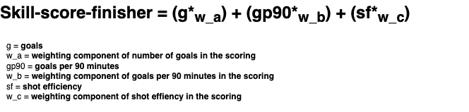
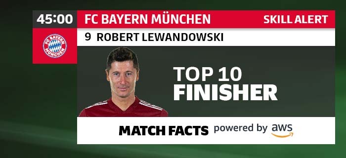
Finisher
A finisher is a player who is exceptionally good at scoring goals. He has a high shot efficiency and accomplishes many goals respective to his playing time. The skill is based on actual goals scored and its difference to expected goals (xGoals). This allows us to evaluate whether chances are being well exploited. Let’s assume that two strikers have the same number of goals. Are they equally strong? Or does one of them score from easy circumstances while the other one finishes in challenging situations? With shot efficiency, this can be answered: if the goals scored exceed the number of xGoals, a player is over-performing and is a more efficient shooter than average. Through the magnitude of this difference, we can quantify the extent to which a shooter’s efficiency beats the average.
The skill score is calculated with the following formula:
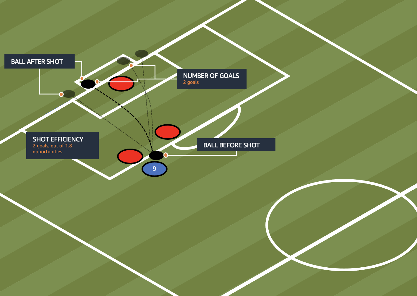
For the finisher, we focus more on goals. The following table gives a closer look at the current top three.
| .. | Goals | GoalsPer90 | ShotEfficiency | Final Score |
| Robert Lewandowski – Rank 1 | 24 | 1.14 | 1.55 | 0.813 |
| Erling Haaland – Rank 2 | 16 | 1.18 | 5.32 | 0.811 |
| Patrik Schick – Rank 3 | 18 | 1.10 | 4.27 | 0.802 |
Robert Lewandowski has scored 24 goals this season, which puts him in first place. Although Haaland has a higher shot efficiency, it’s still not enough for Haaland to be ranked first, because we give higher weighting to goals scored. This indicates that Lewandowski profits highly from both the quality and quantity of received assists, even though he scores exceptionally well. Patrick Schick has scored two more goals than Haaland, but has a lower goal per 90 minutes rate and a lower shot efficiency.
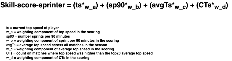
Sprinter
The sprinter has the physical ability to reach high top speeds, and do so more often than others. For this purpose, we evaluate average top speeds across all games of a player’s current season and include the frequency of sprints per 90 minutes, among other metrics. A sprint is counted if a player runs at a minimum pace of 4.0 m/s for more than two seconds, and reaches a peak velocity of at least 6.3 m/s during this time. The duration of the sprint is characterized by the time between the first and last time the 6.3 m/s threshold is reached, and needs to be at least 1 second long to be acknowledged. A new sprint can only be considered to have occurred after the pace had fallen below the 4.0 m/s threshold again.
The skill score is calculated with the following formula:
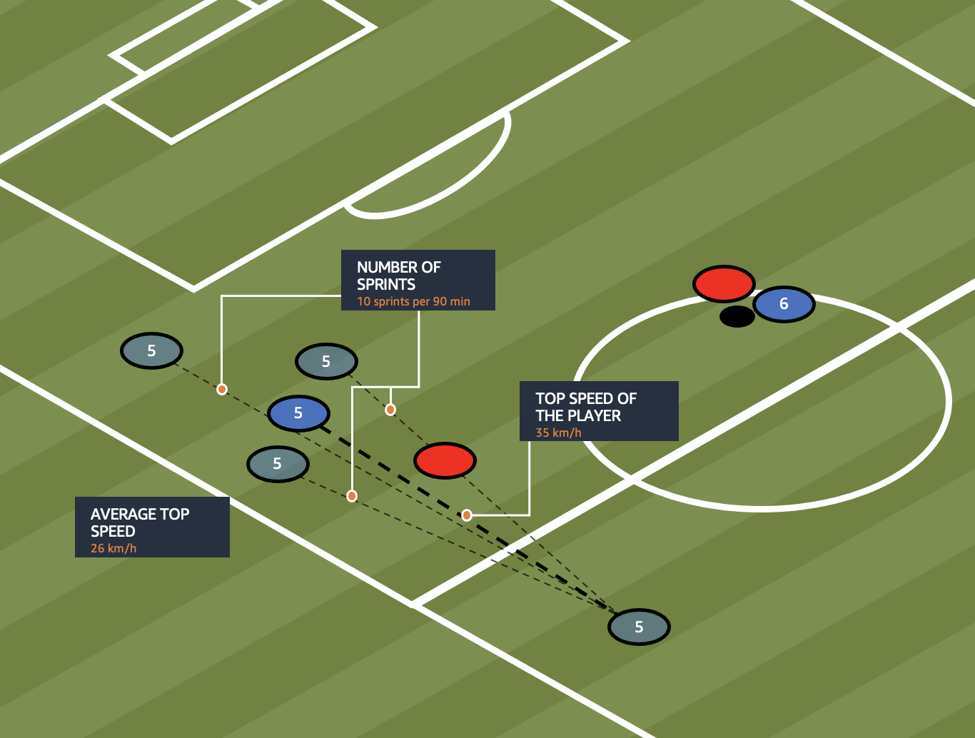
The formula allows us to evaluate the many ways we can look at sprints by players, and go further than just looking at the top speeds these players produce. For example, Jeremiah St. Juste has the current season record of 36.65 km/h. However, if we look at the frequency of his sprints, we find he only sprints nine times on average per match! Alphonso Davies on the other hand might not be as fast as St. Juste (top speed 36.08 km/h), but performs a staggering 31 sprints per match! He sprints much more frequently at with a much higher average speed, opening up space for his team on the pitch.
Ball winner
A player with this ability causes ball losses to the opposing team, both in total and respective to his playing time. He wins a high number of ground and aerial duels, and he steals or intercepts the ball often, creating a safe ball control himself, and a possibility for his team to counterattack.
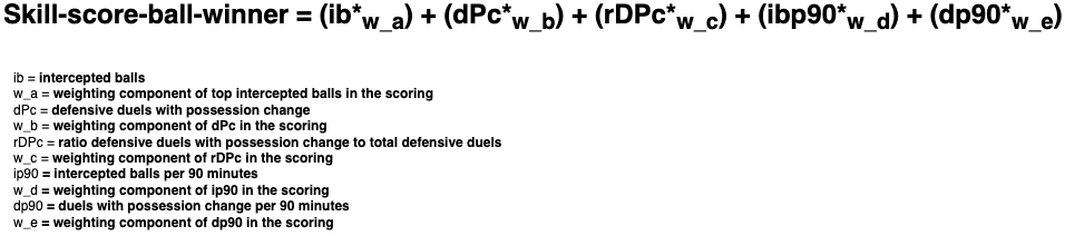
The skill score is calculated with the following formula:
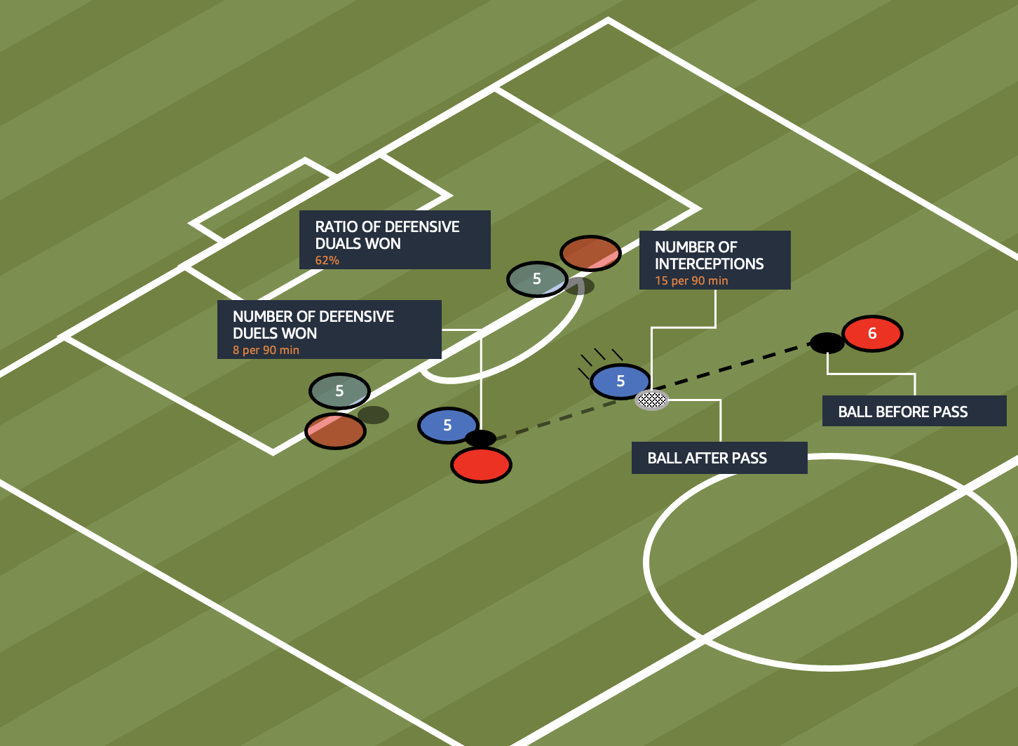
As of this writing, the first place ball winner is Danilo Soares. He has a total of 235 defensive duels. Of the 235 defensive duels, he has won 75, defeating opponents in a face-off. He has intercepted 51 balls this season in his playing position as a defensive back, giving him a win rate of about 32%. On average, he intercepted 2.4 balls per 90 minutes.
Skill example
The Skill Bundesliga Match Fact enables us to unveil abilities and strengths of Bundesliga players. The Skill rankings put players in the spotlight that might have gone unnoticed before in rankings of conventional statistics like goals. For example, take a player like Michael Gregoritsch. Gregoritsch is a striker for FC Augsburg who placed sixth in the finisher ranking as of matchday 21. He has scored five goals so far, which wouldn’t put him at the top of any goal scoring ranking. However, he managed to do this in only 663 minutes played! One of these goals was the late equalizer in the 97th minute that helped Augsburg to avoid the away loss in Berlin.
Through the Skill Bundesliga Match Fact, we can also recognize various qualities of each player. One example of this is the Dortmund star Erling Haaland, who has also earned the badge of sprinter and finisher, and is currently placed sixth amongst Bundesliga sprinters.
 |
 |
 |
 |
All of these metrics are based on player movement data, goal-related data, ball action-related data, and pass-related data. We process this information in data pipelines and extract the necessary relevant statistics per skill, allowing us to calculate the development of all metrics in real time. Many of the aforementioned statistics are normalized by time on the pitch, allowing for the consideration of players who have little playing time but perform amazingly well when they play. The combinations and weights of the metrics are combined into a single score. The result is a ranking for all players on the four player skills. Players ranking in the top 10 receive a skill badge to help fans quickly identify the exceptional qualities they bring to their squads.


Implementation and architecture
Bundesliga Match Facts that have been developed up to this point are independent from one another and rely only on the ingestion of positional and event data, as well as their own calculations. However, this changes for the new Bundesliga Match Fact Skill, which calculates skill rankings based on data produced by existing Match Facts, as for example xGoals or xPass. The outcome of one event, possibly an incredible goal with low chances of going in, can have a significant impact on the finisher skill ranking. Therefore, we built an architecture that always provides the most up-to-date skill rankings whenever there is an update to the underlying data. To achieve real-time updates to the skills, we use Amazon MSK, a managed AWS service for Apache Kafka, as a data streaming and messaging solution. This way, different Bundesliga Match Facts can communicate the latest events and updates in real time.
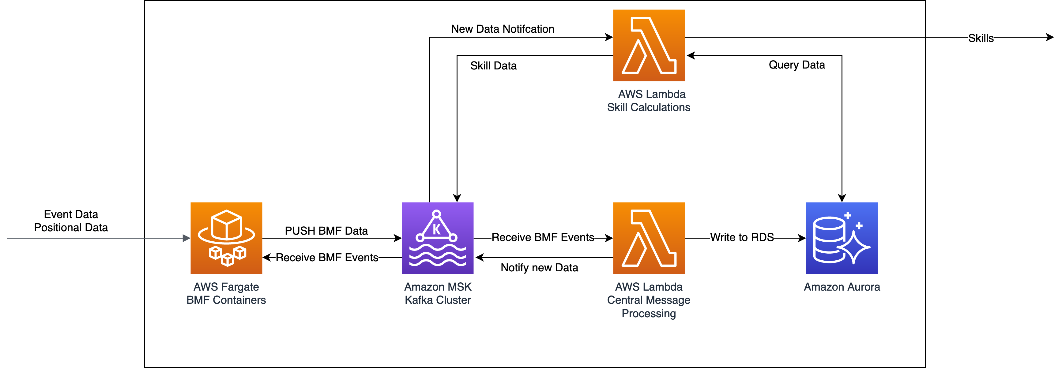
The underlying architecture for Skill consists of four main parts:
- An Amazon Aurora Serverless cluster stores all outputs of existing match facts. This includes, for example, data for each pass (such as xPass, player, intended receiver) or shot (xGoal, player, goal) that has happened since the introduction of Bundesliga Match Facts.
- A central AWS Lambda function writes the Bundesliga Match Fact outputs into the Aurora database and notifies other components that there has been an update.
- A Lambda function for each individual skill computes the skill ranking. These functions run whenever new data is available for the calculation of the specific skill.
- An Amazon MSK Kafka cluster serves as a central point of communication between all these components.
The following diagram illustrates this workflow. Each Bundesliga Match Fact immediately sends an event message to Kafka whenever there is an update to an event (such as an updated xGoals value for a shot event). The central dispatcher Lambda function is automatically triggered whenever a Bundesliga Match Fact sends such a message and writes this data to the database. Then it sends another message via Kafka containing the new data back to Kafka, which serves as a trigger for the individual skill calculation functions. These functions use data from this trigger event, as well as the underlying Aurora cluster, to calculate and publish the newest skill rankings. For a more in-depth look into the use of Amazon MSK within this project, refer to the Set Piece Threat blogpost.
Summary
In this post, we demonstrated how the new Bundesliga Match Fact Skill makes it possible to objectively compare Bundesliga players on four core player dimensions, building on and combining former independent Bundesliga Match Facts in real time. This allows commentators and fans alike to uncover previously unnoticed player abilities and shed light on the roles that various Bundesliga players fulfill.
The new Bundesliga Match Fact is the result of an in-depth analysis by the Bundesliga’s football experts and AWS data scientists to distill and categorize football player qualities based on objective performance data. Player skill badges are shown in the lineup and on player detail pages in the Bundesliga app. In the broadcast, player skills are provided to commentators through the data story finder and visually shown to fans at player substitution and when a player moves up into the respective top 10 ranking.
We hope that you enjoy this brand-new Bundesliga Match Fact and that it provides you with new insights into the game. To learn more about the partnership between AWS and Bundesliga, visit Bundesliga on AWS!
About the Authors
Simon Rolfes played 288 Bundesliga games as a central midfielder, scored 41 goals and won 26 caps for Germany. Currently Rolfes serves as Sporting Director at Bayer 04 Leverkusen where he oversees and develops the pro player roster, the scouting department and the club’s youth development. Simon also writes weekly columns on Bundesliga.com about the latest Bundesliga Match Facts powered by AWS
Luuk Figdor is a Senior Sports Technology Specialist in the AWS Professional Services team. He works with players, clubs, leagues, and media companies such as the Bundesliga and Formula 1 to help them tell stories with data using machine learning. In his spare time, he likes to learn all about the mind and the intersection between psychology, economics, and AI.
Pascal Kühner is a Cloud Application Developer in the AWS Professional Services Team. He works with customers across industries to help them achieve their business outcomes via application development, DevOps, and infrastructure. He is very passionate about sports and enjoys playing basketball and football in his spare time.
Tareq Haschemi is a consultant within AWS Professional Services. His skills and areas of expertise include application development, data science, machine learning, and big data. Based in Hamburg, he supports customers in developing data-driven applications within the cloud. Prior to joining AWS, he was also a consultant in various industries such as aviation and telecommunications. He is passionate about enabling customers on their data/AI journey to the cloud.
Jakub Michalczyk is a Data Scientist at Sportec Solutions AG. Several years ago, he chose math studies over playing football, as he came to the conclusion, he was not good enough at the latter. Now he combines both these passions in his professional career by applying machine learning methods to gain a better insight into this beautiful game. In his spare time, he still enjoys playing seven-a-side football, watching crime movies, and listening to film music.
Javier Poveda-Panter is a Data Scientist for EMEA sports customers within the AWS Professional Services team. He enables customers in the area of spectator sports to innovate and capitalize on their data, delivering high-quality user and fan experiences through machine learning and data science. He follows his passion for a broad range of sports, music, and AI in his spare time.
Podsplainer: What’s a Recommender System? NVIDIA’s Even Oldridge Breaks It Down
The very thing that makes the internet so useful to so many people — the vast quantity of information that’s out there — can also make going online frustrating.
There’s so much available that the sheer volume of choices can be overwhelming. That’s where recommender systems come in, explains NVIDIA AI Podcast host Noah Kravitz.
To dig into how recommender systems work — and why these systems are being harnessed by companies in industries around the globe — Kravitz spoke to Even Oldridge, senior manager for the Merlin team at NVIDIA.
Some highlights, below. For the full conversation we, um, recommend you tune in to the podcast.
Question: So what’s a recommender system and why are they important?
Oldridge: Recommender systems are ubiquitous, and they’re a huge part of the internet and of most mobile apps, and really, most places have interaction that a person has with a computer. A recommender system, at its heart, is a system for taking the vast amount of options available in the world and boiling them down to something that’s relevant to the user in that time or in that context.
That’s a really significant challenge, both from the engineering side and the systems and the models that need to be built. Recommender systems, in my mind, are one of the most complex and significant machine learning challenges of our day. You’re trying to represent what a user like a real live human person is interested in at any given moment. And that’s not an easy thing to do, especially when that person may or may not know what they want.
Question: So broadly speaking, how would you define a recommender system?
Oldridge: A recommender system is a sort of machine learning algorithm that filters content. So you can query the recommender system to narrow down the possible options within a particular context. The classic view that most people have with recommender systems is online shopping, where you’re browsing for a particular item, and you’re seeing other items that are potentially useful in that same context or similar content. And, with sites like Netflix and Spotify and content distributors, you’re seeing content based on the content that you’ve viewed in the past. The recommender system’s role is to try and build a summary of your interests and try to come up with the next relevant thing to show you.
Question: In these different examples that you talked about, do they generally operate the same way across different shopping sites or content sites that users might go to? Or are there different ways of approaching the problem?
Oldridge: There are patterns to the problem, but it’s one of the more fragmented industries, I think. If you look at things like computer vision or natural language processing, there are open-source datasets that have allowed for a lot of significant advancements in the field and allowed for standardization and benchmarking, and those fields have become pretty standardized because of that. In the recommender system space, the interaction data that your users are generating is part of the core value of your company, so most companies are reticent to reveal that data. So there aren’t a lot of great public recommender system datasets out there.
Question: What are you doing at NVIDIA? How did NVIDIA get into the business of recommender systems? What role does your team play?
Oldridge: Why NVIDIA is interested in the business of recommender systems, is, to quote Jensen [Huang, NVIDIA’s CEO], that recommender systems are the most important algorithm on the internet, and they drive a lot of the financial and compute decisions that are being made. For NVIDIA, it’s a very interesting machine learning workload that I think previously has been more applicable to the CPU or has been done more on the CPU.
We’ve gotten to a place where recommender systems on GPUs make a ton of sense. There aren’t many people who are trying to run large natural language processing models or large computer vision models on a CPU. For recsys, there’s a lot of people still focused on the CPU-based solutions. There’s a strong motivation for us to get this right because we have a vested interest in selling GPUs, but beyond that, there’s a similar degree of acceleration that’s possible that led to the revolutions that have happened in computer vision and NLP. When things can happen 10 times faster, then you’re able to do much more exploration and much more diving into the problem space. The field begins to take off in a way that it hasn’t before, and that’s something that our team is really focused on: How we can enable these teams to develop recommender systems much more quickly and efficiently, both from the compute time perspective and making sure that you can develop features and train models and deploy to production really quickly and easily.
Question: How do you judge the effectiveness of a recommender system?
Oldridge: There’s a wide variety of factors that are used to determine and compare the effectiveness, both offline when you’re developing the model and trying to evaluate its performance, and online when you’re running the model in production and the model serving the customer. There’s a lot of metrics in that space. I don’t think there’s any one clear answer of what you need to measure. I think a lot of different companies are, at the heart of it, trying to measure longer-term user engagement, but that’s a very lagging signal. So you need to tie it to metrics that are much more immediate, like interaction and clicks on items, etc.
Question: Could one way to judge it potentially be something like the number of Amazon purchases a user ends up returning?
Oldridge: I think many companies will track those and other forms of user engagement, which can be both positive and negative. Those cost the company a lot, so they’re probably being weighed. It’s very difficult to trace those all the way back to an individual recommendation right at the start. It becomes one of the most interesting and complex challenges — at its heart, a recommender system is trying to model your preference. The preference of a human being in the world is based on their myriad of contexts. That context can change in ways that the model has no idea about. For example, on this podcast, you could tell me about an interesting book that you’ve read and that will lead me to look it up on Amazon and potentially order it. That recommendation from you as a human is you using your context that you have about me and about our conversation and about a bunch of other factors. The system doesn’t know that conversation has happened, so it doesn’t know that that’s kind of something that’s of particular relevance to me.
Question: Tell us about your background?
Oldridge: I did a Ph.D. in computer vision from the University of British Columbia here in Vancouver where I live, and that was pre deep learning. Everything that I did in my Ph.D. could be summarized in probably five lines of TensorFlow at this point.
I went from that role to a job at Plenty of Fish, an online dating site. There were about 30 people when I joined, and the founder had written all of the algorithms that were doing the recommendations. I was the first data science hire and built that up. It was recommending humans to humans for online dating. It’s a very interesting space; it’s a funny one in the sense that the users are the items, and it’s reciprocal. It was a very interesting place to be — you leave work on a Friday night and head home, and there were probably 50,000 or 100,000 people out on a date because of an algorithm. It’s very strange to think about the number of potential new humans that are in the world — marriages, whatever else that just happened — because of these algorithms.
It was interesting, and the data was driving it all. It was my first foray into recommender systems. Then, I left Plenty of Fish and went into deep learning and fast AI. I took six months off when I left Plenty of Fish after it was sold to Match Group, and I spent time really getting into deep learning, which I hadn’t spent any time on, and I got deep into that through the fast AI course.
Question: You mentioned that NVIDIA has some tools available to make it easier for smaller organizations. For anybody who wants to build a recommender system, do you want to speak to any of the specific things that are out there? Or maybe tools that you’re working on with the Merlin team that folks can use?
Oldridge: The Merlin team consists largely of people like myself, who’ve built recommender systems in production in the past and understand the pain of it. It’s really hard to build a recommender system.
We’re working on three main premises:
- Make it work: We want to have a framework that provides end-to-end recommendations, so you can complete all the different stages and all the things you need.
- Make it easy: It should be straightforward to be able to do things that are commonly done within the space. We’re really thinking about issues such as, “Where was a pain point in our past where it was a real challenge to use the existing tooling? And how can we smooth that pain point over?”
- Make it fast: At NVIDIA, we want to make sure that this is performance, at scale, and how these things scale is an incredibly important part of the problem space.
Question: Where do you see the space headed over the next couple of years?
Oldridge: What we’re hoping to do with Merlin is provide a standard set of tools and a standard framework that everyone can use and think about to be able to do accelerated recommender systems. Especially as we accelerate things by a 10x factor or more as it changes the pattern.
One of my favorite diagrams that I saw since joining NVIDIA was the diagram of the developer, who, at the start of their day, gets a coffee and then starts [a data science project] and then goes to get another coffee because that takes so long and kind of just this back and forth, you know, drinking six or 10 cups. And, getting to the point where you know, they can do basically three things in a day.
It hits home because that was me a couple years ago, and I was personally facing that. It was so frustrating because I wanted to get stuff done, but because of that lagging signal, you’re not nearly as effective when you get back to it to try and dig in. Seeing the difference that it makes when it gets to that 1-to-3-minute cycle where you’re running something and getting the results and running something and getting the results and you get into that flow pattern, you’re really able to explore things quickly. Then you get to the point where you’re iterating so quickly, and then you can start leveraging the parallelization that happens on the GPU and begin to scale things up.
Question: For the folks who want to find out more about the work you’re doing and what’s going on with Merlin, where can they go online to learn more or dig a little deeper into some white papers and some of the more technical aspects of the work?
Oldridge: A great starting point is our GitHub. We linked out to a bunch of our papers there. I have a bunch of talks that I’ve given about Merlin across various sources. If you search for my name in YouTube, or for Merlin recommender systems, there’s a lot of information you can find out there.
Subscribe to the AI Podcast: Now Available on Amazon Music
You can now listen to the AI Podcast through Amazon Music.
You can also get the AI Podcast through iTunes, Google Podcasts, Google Play, Castbox, DoggCatcher, Overcast, PlayerFM, Pocket Casts, Podbay, PodBean, PodCruncher, PodKicker, Soundcloud, Spotify, Stitcher and TuneIn.
Make the AI Podcast better: Have a few minutes to spare? Fill out our listener survey.
The post Podsplainer: What’s a Recommender System? NVIDIA’s Even Oldridge Breaks It Down appeared first on NVIDIA Blog.
Understanding LazyTensor System Performance with PyTorch/XLA on Cloud TPU
Introduction
Ease of use, expressivity, and debuggability are among the core principles of PyTorch. One of the key drivers for the ease of use is that PyTorch execution is by default “eager, i.e. op by op execution preserves the imperative nature of the program. However, eager execution does not offer the compiler based optimization, for example, the optimizations when the computation can be expressed as a graph.
LazyTensor [1], first introduced with PyTorch/XLA, helps combine these seemingly disparate approaches. While PyTorch eager execution is widely used, intuitive, and well understood, lazy execution is not as prevalent yet.
In this post we will explore some of the basic concepts of the LazyTensor System with the goal of applying these concepts to understand and debug performance of LazyTensor based implementations in PyTorch. Although we will use PyTorch/XLA on Cloud TPU as the vehicle for exploring these concepts, we hope that these ideas will be useful to understand other system(s) built on LazyTensors.
LazyTensor
Any operation performed on a PyTorch tensor is by default dispatched as a kernel or a composition of kernels to the underlying hardware. These kernels are executed asynchronously on the underlying hardware. The program execution is not blocked until the value of a tensor is fetched. This approach scales extremely well with massively parallel programmed hardware such as GPUs.
The starting point of a LazyTensor system is a custom tensor type. In PyTorch/XLA, this type is called XLA tensor. In contrast to PyTorch’s native tensor type, operations performed on XLA tensors are recorded into an IR graph. Let’s examine an example that sums the product of two tensors:
import torch
import torch_xla
import torch_xla.core.xla_model as xm

dev = xm.xla_device()

x1 = torch.rand((3, 3)).to(dev)
x2 = torch.rand((3, 8)).to(dev)

y1 = torch.einsum('bs,st->bt', x1, x2)
print(torch_xla._XLAC._get_xla_tensors_text([y1]))
You can execute this colab notebook to examine the resulting graph for y1. Notice that no computation has been performed yet.
y1 = y1 + x2
print(torch_xla._XLAC._get_xla_tensors_text([y1]))
The operations will continue until PyTorch/XLA encounters a barrier. This barrier can either be a mark step() api call or any other event which forces the execution of the graph recorded so far.
xm.mark_step()
print(torch_xla._XLAC._get_xla_tensors_text([y1]))
Once the mark_step() is called, the graph is compiled and then executed on TPU, i.e. the tensors have been materialized. Therefore, the graph is now reduced to a single line y1 tensor which holds the result of the computation.
Compile Once, Execute Often
XLA compilation passes offer optimizations (e.g. op-fusion, which reduces HBM pressure by using scratch-pad memory for multiple ops, ref ) and leverages lower level XLA infrastructure to optimally use the underlying hardware. However, there is one caveat, compilation passes are expensive, i.e. can add to the training step time. Therefore, this approach scales well if and only if we can compile once and execute often (compilation cache helps, such that the same graph is not compiled more than once).
In the following example, we create a small computation graph and time the execution:
y1 = torch.rand((3, 8)).to(dev)
def dummy_step() :
  y1 = torch.einsum('bs,st->bt', y1, x)
  xm.mark_step()
  return y1
%timeit dummy_step
The slowest run took 29.74 times longer than the fastest. This could mean that an intermediate result is being cached.
10000000 loops, best of 5: 34.2 ns per loop
You notice that the slowest step is quite longer than the fastest. This is because of the graph compilation overhead which is incurred only once for a given shape of graph, input shape, and output shape. Subsequent steps are faster because no graph compilation is necessary.
This also implies that we expect to see performance cliffs when the “compile once and execute often” assumption breaks. Understanding when this assumption breaks is the key to understanding and optimizing the performance of a LazyTensor system. Let’s examine what triggers the compilation.
Graph Compilation and Execution and LazyTensor Barrier
We saw that the computation graph is compiled and executed when a LazyTensor barrier is encountered. There are three scenarios when the LazyTensor barrier is automatically or manually introduced. The first is the explicit call of mark_step() api as shown in the preceding example. mark_step() is also called implicitly at every step when you wrap your dataloader with MpDeviceLoader (highly recommended to overlap compute and data upload to TPU device). The Optimizer step method of xla_model also allows to implicitly call mark_step (when you set barrier=True).
The second scenario where a barrier is introduced is when PyTorch/XLA finds an op with no mapping (lowering) to equivalent XLA HLO ops. PyTorch has 2000+ operations. Although most of these operations are composite (i.e. can be expressed in terms of other fundamental operations), some of these operations do not have corresponding lowering in XLA.
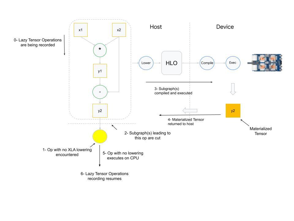
What happens when an op with no XLA lowering is used? PyTorch XLA stops the operation recording and cuts the graph(s) leading to the input(s) of the unlowered op. This cut graph is then compiled and dispatched for execution. The results (materialized tensor) of execution are sent back from device to host, the unlowered op is then executed on the host (cpu), and then downstream LazyTensor operations creating a new graph(s) until a barrier is encountered again.
The third and final scenario which results in a LazyTensor barrier is when there is a control structure/statement or another method which requires the value of a tensor. This statement would at the minimum cause the execution of the computation graph leading to the tensor (if the graph has already been seen) or cause compilation and execution of both.
Other examples of such methods include .item(), isEqual(). In general, any operation that maps Tensor -> Scalar will cause this behavior.
Dynamic Graph
As illustrated in the preceding section, graph compilation cost is amortized if the same shape of the graph is executed many times. It’s because the compiled graph is cached with a hash derived from the graph shape, input shape, and the output shape. If these shapes change it will trigger compilation, and too frequent compilation will result in training time degradation.
Let’s consider the following example:
def dummy_step(x, y, loss, acc=False):
  z = torch.einsum('bs,st->bt', y, x)
  step_loss = z.sum().view(1,)
  if acc:
    loss = torch.cat((loss, step_loss))
  else:
    loss = step_loss
  xm.mark_step()
  return loss


import time
def measure_time(acc=False):
  exec_times = []
  iter_count = 100
  x = torch.rand((512, 8)).to(dev)
  y = torch.rand((512, 512)).to(dev)
  loss = torch.zeros(1).to(dev)
  for i in range(iter_count):
    tic = time.time()
    loss = dummy_step(x, y, loss, acc=acc)
    toc = time.time()
    exec_times.append(toc - tic)
  return exec_times

dyn = measure_time(acc=True) # acc= True Results in dynamic graph
st = measure_time(acc=False) # Static graph, computation shape, inputs and output shapes don't change

import matplotlib.pyplot as plt
plt.plot(st, label = 'static graph')
plt.plot(dyn, label = 'dynamic graph')
plt.legend()
plt.title('Execution time in seconds')
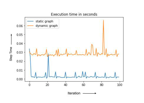
Note that static and dynamic cases have the same computation but dynamic graph compiles every time, leading to the higher overall run-time. In practice, the training step with recompilation can sometimes be an order of magnitude or slower. In the next section we discuss some of the PyTorch/XLA tools to debug training degradation.
Profiling Training Performance with PyTorch/XLA
PyTorch/XLA profiling consists of two major components. First is the client side profiling. This feature is turned on by simply setting the environment variable PT_XLA_DEBUG to 1. Client side profiling points to unlowered ops or device-to-host transfer in your source code. Client side profiling also reports if there are too frequent compilations happening during the training. You can explore some metrics and counters provided by PyTorch/XLA in conjunction with the profiler in this notebook.
The second component offered by PyTorch/XLA profiler is the inline trace annotation. For example:
import torch_xla.debug.profiler as xp

def train_imagenet():
  print('==> Preparing data..')
  img_dim = get_model_property('img_dim')
  ....
  server = xp.start_server(3294)
  def train_loop_fn(loader, epoch):
    ....
    model.train()
    for step, (data, target) in enumerate(loader):
      with xp.StepTrace('Train_Step', step_num=step):
        ....
        if FLAGS.amp:
        ....
        else:
          with xp.Trace('build_graph'):
            output = model(data)
            loss = loss_fn(output, target)
            loss.backward()
          xm.optimizer_step(optimizer)
Notice the start_server api call. The port number that you have used here is the same port number you will use with the tensorboard profiler in order to view the op trace similar to:
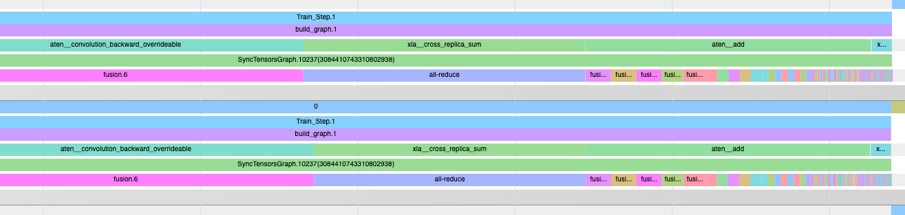
Op trace along with the client-side debugging function is a powerful set of tools to debug and optimize your training performance with PyTorch/XLA. For more detailed instructions on the profiler usage, the reader is encouraged to explore blogs part-1, part-2, and part-3 of the blog series on PyTorch/XLA performance debugging.
Summary
In this article we have reviewed the fundamentals of the LazyTensor system. We built on those fundamentals with PyTorch/XLA to understand the potential causes of training performance degradation. We discussed why “compile once and execute often” helps to get the best performance on LazyTensor systems, and why training slows down when this assumption breaks.
We hope that PyTorch users will find these insights helpful for their novel works with LazyTensor systems.
Acknowledgements
A big thank you to my outstanding colleagues Jack Cao, Milad Mohammedi, Karl Weinmeister, Rajesh Thallam, Jordan Tottan (Google) and Geeta Chauhan (Meta) for their meticulous reviews and feedback. And thanks to the extended PyTorch/XLA development team from Google, Meta, and the open source community to make PyTorch possible on TPUs. And finally, thanks to the authors of the LazyTensor paper not only for developing LazyTensor but also for writing such an accessible paper.