Monthly Archives: August 2022

With personalized content more likely to drive customer engagement, businesses continuously seek to provide tailored content based on their customer’s profile and behavior. Recommendation systems in particular seek to predict the preference an end-user would give to an item. Some common use cases include product recommendations on online retail stores, personalizing newsletters, generating music playlist recommendations, or even discovering similar content on online media services.

However, it can be challenging to create an effective recommendation system due to complexities in model training, algorithm selection, and platform management. Amazon Personalize enables developers to improve customer engagement through personalized product and content recommendations with no machine learning (ML) expertise required. Developers can start to engage customers right away by using captured user behavior data. Behind the scenes, Amazon Personalize examines this data, identifies what is meaningful, selects the right algorithms, trains and optimizes a personalization model that is customized for your data, and provides recommendations via an API endpoint.

Although providing recommendations in real time can help boost engagement and satisfaction, sometimes this might not actually be required, and performing this in batch on a scheduled basis can simply be a more cost-effective and manageable option.

This post shows you how to use AWS services to not only create recommendations but also operationalize a batch recommendation pipeline. We walk through the end-to-end solution without a single line of code. We discuss two topics in detail:

• Preparing your data using AWS Glue
• Orchestrating the Amazon Personalize batch inference jobs using AWS Step Functions

Solution overview

In this solution, we use the MovieLens dataset. This dataset includes 86,000 ratings of movies from 2,113 users. We attempt to use this data to generate recommendations for each of these users.

Data preparation is very important to ensure we get customer behavior data into a format that is ready for Amazon Personalize. The architecture described in this post uses AWS Glue, a serverless data integration service, to perform the transformation of raw data into a format that is ready for Amazon Personalize to consume. The solution uses Amazon Personalize to create batch recommendations for all users by using a batch inference. We then use a Step Functions workflow so that the automated workflow can be run by calling Amazon Personalize APIs in a repeatable manner.

The following diagram demonstrates this solution.

We will build this solution with the following steps:

1. Build a data transformation job to transform our raw data using AWS Glue.
2. Build an Amazon Personalize solution with the transformed dataset.
3. Build a Step Functions workflow to orchestrate the generation of batch inferences.

Prerequisites

You need the following for this walkthrough:

• An AWS account
• Permissions to create new AWS Identity and Access Management (IAM) roles

Build a data transformation job to transform raw data with AWS Glue

With Amazon Personalize, input data needs to have a specific schema and file format. Data from interactions between users and items must be in CSV format with specific columns, whereas the list of users for which you want to generate recommendations for must be in JSON format. In this section, we use AWS Glue Studio to transform raw input data into the required structures and format for Amazon Personalize.

AWS Glue Studio provides a graphical interface that is designed for easy creation and running of extract, transform, and load (ETL) jobs. You can visually create data transformation workloads through simple drag-and-drop operations.

We first prepare our source data in Amazon Simple Storage Service (Amazon S3), then we transform the data without code.

1. On the Amazon S3 console, create an S3 bucket with three folders: raw, transformed, and curated.
2. Download the MovieLens dataset and upload the uncompressed file named user_ratingmovies-timestamp.dat to your bucket under the raw folder.
3. On the AWS Glue Studio console, choose Jobs in the navigation pane.
4. Select Visual with a source and target, then choose Create.
   
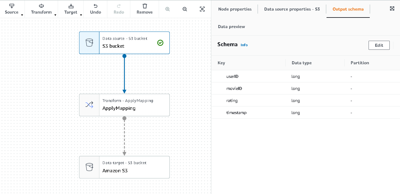
5. Choose the first node called Data source – S3 bucket. This is where we specify our input data.
6. On the Data source properties tab, select S3 location and browse to your uploaded file.
7. For Data format, choose CSV, and for Delimiter, choose Tab.
   
8. We can choose the Output schema tab to verify that the schema has inferred the columns correctly.
9. If the schema doesn’t match your expectations, choose Edit to edit the schema.
   

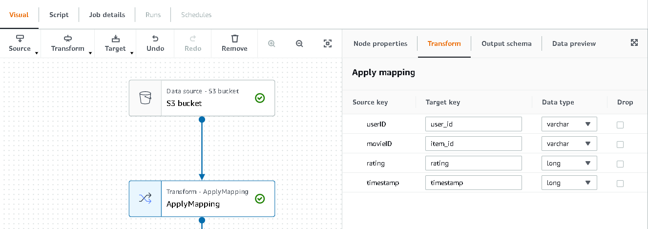
Next, we transform this data to follow the schema requirements for Amazon Personalize.

10. Choose the Transform – Apply Mapping node and, on the Transform tab, update the target key and data types.
    Amazon Personalize, at minimum, expects the following structure for the interactions dataset:

• • user_id (string)
  • item_id (string)
  • timestamp (long, in Unix epoch time format)
    

In this example, we exclude the poorly rated movies in the dataset.

11. To do so, remove the last node called S3 bucket and add a filter node on the Transform tab.
12. Choose Add condition and filter out data where rating < 3.5.
    

We now write the output back to Amazon S3.

13. Expand the Target menu and choose Amazon S3.
14. For S3 Target Location, choose the folder named transformed.
15. Choose CSV as the format and suffix the Target Location with interactions/.

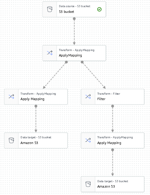
Next, we output a list of users that we want to get recommendations for.

16. Choose the ApplyMapping node again, and then expand the Transform menu and choose ApplyMapping.
17. Drop all fields except for user_id and rename that field to userId. Amazon Personalize expects that field to be named userId.
18. Expand the Target menu again and choose Amazon S3.
19. This time, choose JSON as the format, and then choose the transformed S3 folder and suffix it with batch_users_input/.

This produces a JSON list of users as input for Amazon Personalize. We should now have a diagram that looks like the following.

We are now ready to run our transform job.

20. On the IAM console, create a role called glue-service-role and attach the following managed policies:
    • AWSGlueServiceRole
    • AmazonS3FullAccess

For more information on how to create IAM service roles, refer to the Creating a role to delegate permissions to an AWS service.

21. Navigate back to your AWS Glue Studio job, and choose the Job details tab.
22. Set the job name as batch-personalize-input-transform-job.
23. Choose the newly created IAM role.
24. Keep the default values for everything else.
    
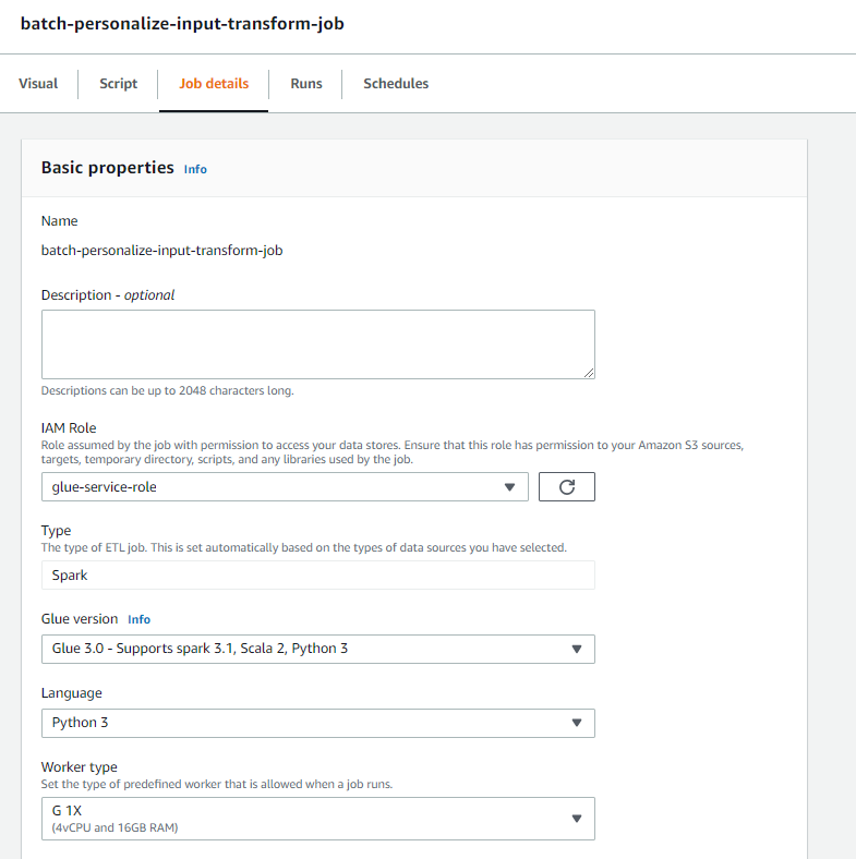
25. Choose Save.
26. When you’re ready, choose Run and monitor the job in the Runs tab.
27. When the job is complete, navigate to the Amazon S3 console to validate that your output file has been successfully created.

We have now shaped our data into the format and structure that Amazon Personalize requires. The transformed dataset should have the following fields and format:

• Interactions dataset – CSV format with fields USER_ID, ITEM_ID, TIMESTAMP
• User input dataset – JSON format with element userId

Build an Amazon Personalize solution with the transformed dataset

With our interactions dataset and user input data in the right format, we can now create our Amazon Personalize solution. In this section, we create our dataset group, import our data, and then create a batch inference job. A dataset group organizes resources into containers for Amazon Personalize components.

1. On the Amazon Personalize console, choose Create dataset group.
2. For Domain, select Custom.
3. Choose Create dataset group and continue.
   

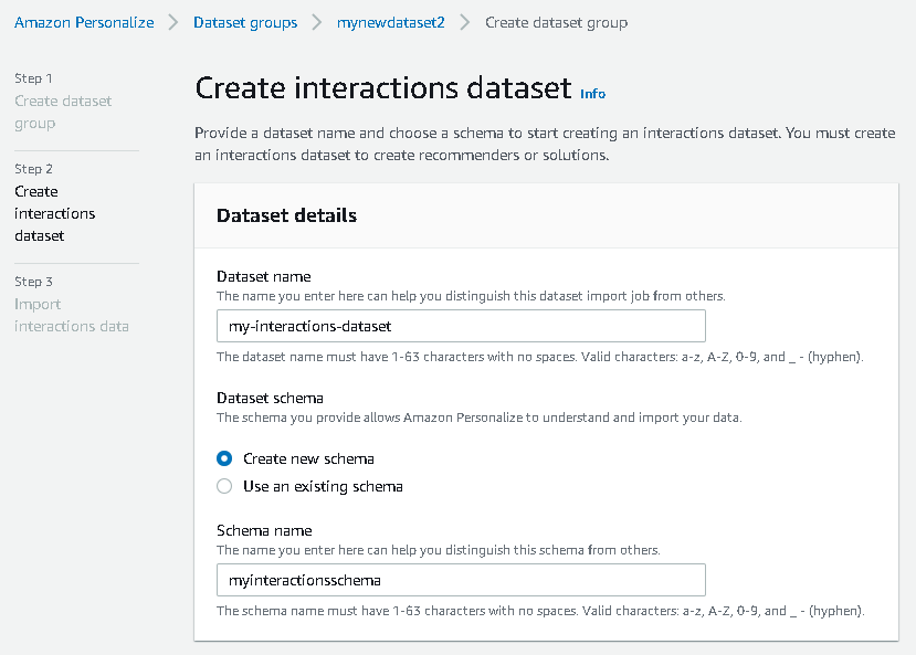
Next, create the interactions dataset.

4. Enter a dataset name and select Create new schema.
5. Choose Create dataset and continue.
   

We now import the interactions data that we had created earlier.

6. Navigate to the S3 bucket in which we created our interactions CSV dataset.
7. On the Permissions tab, add the following bucket access policy so that Amazon Personalize has access. Update the policy to include your bucket name.

   {
      "Version":"2012-10-17",
      "Id":"PersonalizeS3BucketAccessPolicy",
      "Statement":[
         {
            "Sid":"PersonalizeS3BucketAccessPolicy",
            "Effect":"Allow",
            "Principal":{
               "Service":"personalize.amazonaws.com"
            },
            "Action":[
               "s3:GetObject",
               "s3:ListBucket",
               "s3:PutObject"
            ],
            "Resource":[
               "arn:aws:s3:::<your-bucket-name>",
               "arn:aws:s3:::<your-bucket-name> /*"
            ]
         }
      ]
   }

Navigate back to Amazon Personalize and choose Create your dataset import job. Our interactions dataset should now be importing into Amazon Personalize. Wait for the import job to complete with a status of Active before continuing to the next step. This should take approximately 8 minutes.

8. On the Amazon Personalize console, choose Overview in the navigation pane and choose Create solution.
   
9. Enter a solution name.
10. For Solution type, choose Item recommendation.
11. For Recipe, choose the aws-user-personalization recipe.
12. Choose Create and train solution.
    

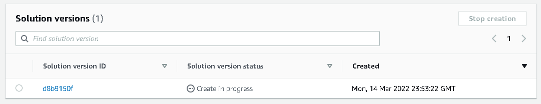
The solution now trains against the interactions dataset that was imported with the user personalization recipe. Monitor the status of this process under Solution versions. Wait for it to complete before proceeding. This should take approximately 20 minutes.

We now create our batch inference job, which generates recommendations for each of the users present in the JSON input.

13. In the navigation pane, under Custom resources, choose Batch inference jobs.
14. Enter a job name, and for Solution, choose the solution created earlier.
15. Choose Create batch inference job.
    
16. For Input data configuration, enter the S3 path of where the batch_users_input file is located.

This is the JSON file that contains userId.

17. For Output data configuration path, choose the curated path in S3.
18. Choose Create batch inference job.

This process takes approximately 30 minutes. When the job is finished, recommendations for each of the users specified in the user input file are saved in the S3 output location.

We have successfully generated a set of recommendations for all of our users. However, we have only implemented the solution using the console so far. To make sure that this batch inferencing runs regularly with the latest set of data, we need to build an orchestration workflow. In the next section, we show you how to create an orchestration workflow using Step Functions.

Build a Step Functions workflow to orchestrate the batch inference workflow

To orchestrate your pipeline, complete the following steps:

1. On the Step Functions console, choose Create State Machine.
2. Select Design your workflow visually, then choose Next.
   
3. Drag the CreateDatasetImportJob node from the left (you can search for this node in the search box) onto the canvas.
4. Choose the node, and you should see the configuration API parameters on the right. Record the ARN.
5. Enter your own values in the API Parameters text box.

This calls the CreateDatasetImportJob API with the parameter values that you specify.

6. Drag the CreateSolutionVersion node onto the canvas.
7. Update the API parameters with the ARN of the solution that you noted down.

This creates a new solution version with the newly imported data by calling the CreateSolutionVersion API.

8. Drag the CreateBatchInferenceJob node onto the canvas and similarly update the API parameters with the relevant values.

Make sure that you use the $.SolutionVersionArn syntax to retrieve the solution version ARN parameter from the previous step. These API parameters are passed to the CreateBatchInferenceJob API.

We need to build a wait logic in the Step Functions workflow to make sure the recommendation batch inference job finishes before the workflow completes.

9. Find and drag in a Wait node.
10. In the configuration for Wait, enter 300 seconds.

This is an arbitrary value; you should alter this wait time according to your specific use case.

11. Choose the CreateBatchInferenceJob node again and navigate to the Error handling tab.
12. For Catch errors, enter Personalize.ResourceInUseException.
13. For Fallback state, choose Wait.

This step enables us to periodically check the status of the job and it only exits the loop when the job is complete.

14. For ResultPath, enter $.errorMessage.

This effectively means that when the “resource in use” exception is received, the job waits for x seconds before trying again with the same inputs.

15. Choose Save, and then choose Start the execution.

We have successfully orchestrated our batch recommendation pipeline for Amazon Personalize. As an optional step, you can use Amazon EventBridge to schedule a trigger of this workflow on a regular basis. For more details, refer to EventBridge (CloudWatch Events) for Step Functions execution status changes.

Clean up

To avoid incurring future charges, delete the resources that you created for this walkthrough.

Conclusion

In this post, we demonstrated how to create a batch recommendation pipeline by using a combination of AWS Glue, Amazon Personalize, and Step Functions, without needing a single line of code or ML experience. We used AWS Glue to prep our data into the format that Amazon Personalize requires. Then we used Amazon Personalize to import the data, create a solution with a user personalization recipe, and create a batch inferencing job that generates a default of 25 recommendations for each user, based on past interactions. We then orchestrated these steps using Step Functions so that we can run these jobs automatically.

For steps to consider next, user segmentation is one of the newer recipes in Amazon Personalize, which you might want to explore to create user segments for each row of the input data. For more details, refer to Getting batch recommendations and user segments.

About the author

Maxine Wee is an AWS Data Lab Solutions Architect. Maxine works with customers on their use cases, designs solutions to solve their business problems, and guides them through building scalable prototypes. Prior to her journey with AWS, Maxine helped customers implement BI, data warehousing, and data lake projects in Australia.

Read More

On August 9, 2022, we announced the general availability of cross-account sharing of Amazon SageMaker Pipelines entities. You can now use cross-account support for Amazon SageMaker Pipelines to share pipeline entities across AWS accounts and access shared pipelines directly through Amazon SageMaker API calls.

Customers are increasingly adopting multi-account architectures for deploying and managing machine learning (ML) workflows with SageMaker Pipelines. This involves building workflows in development or experimentation (dev) accounts, deploying and testing them in a testing or pre-production (test) account, and finally promoting them to production (prod) accounts to integrate with other business processes. You can benefit from cross-account sharing of SageMaker pipelines in the following use cases:

• When data scientists build ML workflows in a dev account, those workflows are then deployed by an ML engineer as a SageMaker pipeline into a dedicated test account. To further monitor those workflows, data scientists now require cross-account read-only permission to the deployed pipeline in the test account.
• ML engineers, ML admins, and compliance teams, who manage deployment and operations of those ML workflows from a shared services account, also require visibility into the deployed pipeline in the test account. They might also require additional permissions for starting, stopping, and retrying those ML workflows.

In this post, we present an example multi-account architecture for developing and deploying ML workflows with SageMaker Pipelines.

Solution overview

A multi-account strategy helps you achieve data, project, and team isolation while supporting software development lifecycle steps. Cross-account pipeline sharing supports a multi-account strategy, removing the overhead of logging in and out of multiple accounts and improving ML testing and deployment workflows by sharing resources directly across multiple accounts.

In this example, we have a data science team that uses a dedicated dev account for the initial development of the SageMaker pipeline. This pipeline is then handed over to an ML engineer, who creates a continuous integration and continuous delivery (CI/CD) pipeline in their shared services account to deploy this pipeline into a test account. To still be able to monitor and control the deployed pipeline from their respective dev and shared services accounts, resource shares are set up with AWS Resource Access Manager in the test and dev accounts. With this setup, the ML engineer and the data scientist can now monitor and control the pipelines in the dev and test accounts from their respective accounts, as shown in the following figure.

In the workflow, the data scientist and ML engineer perform the following steps:

1. The data scientist (DS) builds a model pipeline in the dev account.
2. The ML engineer (MLE) productionizes the model pipeline and creates a pipeline, (for this post, we call it sagemaker-pipeline).
3. sagemaker-pipeline code is committed to an AWS CodeCommit repository in the shared services account.
4. The data scientist creates an AWS RAM resource share for sagemaker-pipeline and shares it with the shared services account, which accepts the resource share.
5. From the shared services account, ML engineers are now able to describe, monitor, and administer the pipeline runs in the dev account using SageMaker API calls.
6. A CI/CD pipeline triggered in the shared service account builds and deploys the code to the test account using AWS CodePipeline.
7. The CI/CD pipeline creates and runs sagemaker-pipeline in the test account.
8. After running sagemaker-pipeline in the test account, the CI/CD pipeline creates a resource share for sagemaker-pipeline in the test account.
9. A resource share from the test sagemaker-pipeline with read-only permissions is created with the dev account, which accepts the resource share.
10. The data scientist is now able to describe and monitor the test pipeline run status using SageMaker API calls from the dev account.
11. A resource share from the test sagemaker-pipeline with extended permissions is created with the shared services account, which accepts the resource share.
12. The ML engineer is now able to describe, monitor, and administer the test pipeline run using SageMaker API calls from the shared services account.

In the following sections, we go into more detail and provide a demonstration on how to set up cross-account sharing for SageMaker pipelines.

How to create and share SageMaker pipelines across accounts

In this section, we walk through the necessary steps to create and share pipelines across accounts using AWS RAM and the SageMaker API.

Set up the environment

First, we need to set up a multi-account environment to demonstrate cross-account sharing of SageMaker pipelines:

1. Set up two AWS accounts (dev and test). You can set this up as member accounts of an organization or as independent accounts.
2. If you’re setting up your accounts as member of an organization, you can enable resource sharing with your organization. With this setting, when you share resources in your organization, AWS RAM doesn’t send invitations to principals. Principals in your organization gain access to shared resources without exchanging invitations.
3. In the test account, launch Amazon SageMaker Studio and run the notebook train-register-deploy-pipeline-model. This creates an example pipeline in your test account. To simplify the demonstration, we use SageMaker Studio in the test account to launch the the pipeline. For real life projects, you should use Studio only in the dev account and launch SageMaker Pipeline in the test account using your CI/CD tooling.

Follow the instructions in the next section to share this pipeline with the dev account.

Set up a pipeline resource share

To share your pipeline with the dev account, complete the following steps:

1. On the AWS RAM console, choose Create resource share.
2. For Select resource type, choose SageMaker Pipelines.
3. Select the pipeline you created in the previous step.
4. Choose Next.
   
5. For Permissions, choose your associated permissions.
6. Choose Next.
   Next, you decide how you want to grant access to principals.
7. If you need to share the pipeline only within your organization accounts, select Allow Sharing only within your organization; otherwise select Allow sharing with anyone.
8. For Principals, choose your principal type (you can use an AWS account, organization, or organizational unit, based on your sharing requirement). For this post, we share with anyone at the AWS account level.
9. Select your principal ID.
10. Choose Next.
    
11. On the Review and create page, verify your information is correct and choose Create resource share.
    
12. Navigate to your destination account (for this post, your dev account).
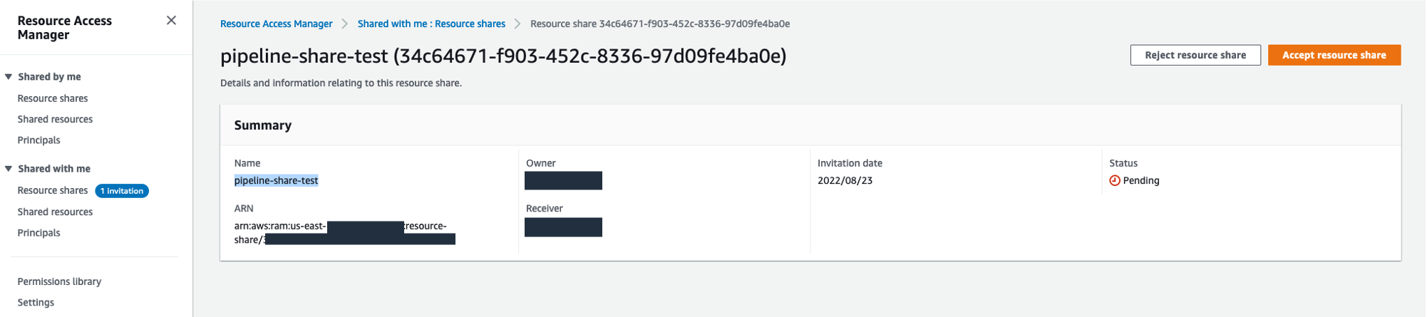
13. On the AWS RAM console, under Shared with me in the navigation pane, choose Resource shares.
14. Choose your resource share and choose Accept resource share.
    

Resource sharing permissions

When creating your resource share, you can choose from one of two supported permission policies to associate with the SageMaker pipeline resource type. Both policies grant access to any selected pipeline and all of its runs.

The AWSRAMDefaultPermissionSageMakerPipeline policy allows the following read-only actions:

"sagemaker:DescribePipeline"
"sagemaker:DescribePipelineDefinitionForExecution"
"sagemaker:DescribePipelineExecution"
"sagemaker:ListPipelineExecutions"
"sagemaker:ListPipelineExecutionSteps"
"sagemaker:ListPipelineParametersForExecution"
"sagemaker:Search"

The AWSRAMPermissionSageMakerPipelineAllowExecution policy includes all of the read-only permissions from the default policy, and also allows shared accounts to start, stop, and retry pipeline runs.

The extended pipeline run permission policy allows the following actions:

"sagemaker:DescribePipeline"
"sagemaker:DescribePipelineDefinitionForExecution"
"sagemaker:DescribePipelineExecution"
"sagemaker:ListPipelineExecutions"
"sagemaker:ListPipelineExecutionSteps"
"sagemaker:ListPipelineParametersForExecution"
"sagemaker:StartPipelineExecution"
"sagemaker:StopPipelineExecution"
"sagemaker:RetryPipelineExecution"
"sagemaker:Search"

Access shared pipeline entities through direct API calls

In this section, we walk through how you can use various SageMaker Pipeline API calls to gain visibility into pipelines running in remote accounts that have been shared with you. For testing the APIs against the pipeline running in the test account from the dev account, log in to the dev account and use AWS CloudShell.

For the cross-account SageMaker Pipeline API calls, you always need to use your pipeline ARN as the pipeline identification. That also includes the commands requiring the pipeline name, where you need to use your pipeline ARN as the pipeline name.

To get your pipeline ARN, in your test account, navigate to your pipeline details in Studio via SageMaker Resources.

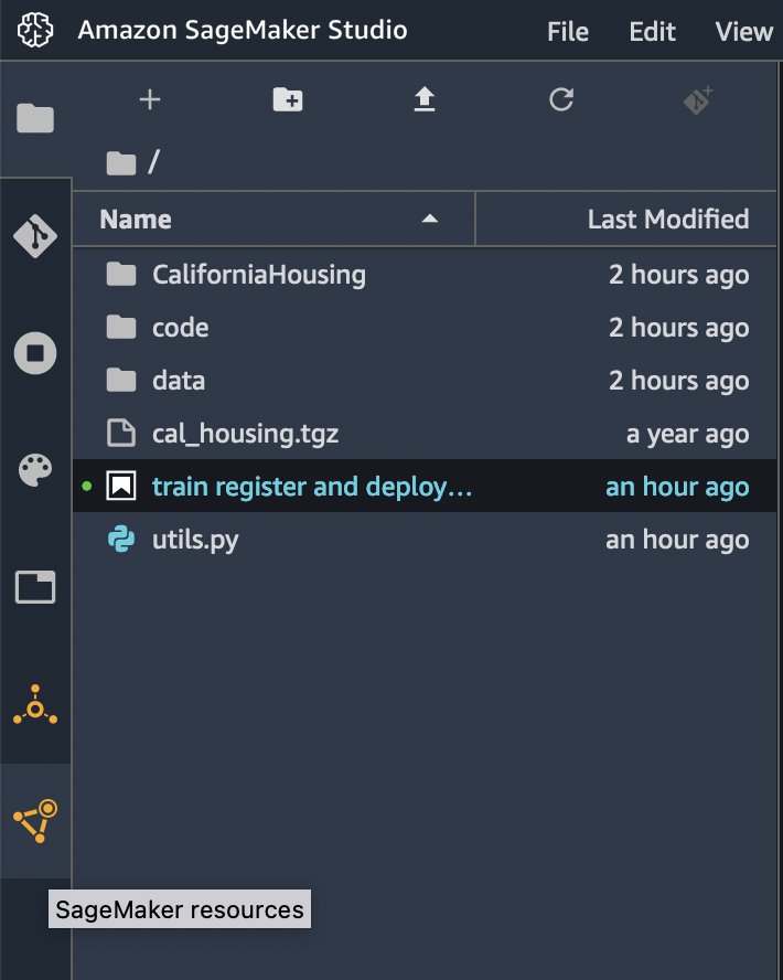
Choose Pipelines on your resources list.

Choose your pipeline and go to your pipeline Settings tab. You can find the pipeline ARN with your Metadata information. For this example, your ARN is defined as "arn:aws:sagemaker:us-east-1:<account-id>:pipeline/serial-inference-pipeline".

ListPipelineExecutions

This API call lists the runs of your pipeline. Run the following command, replacing $SHARED_PIPELINE_ARN with your pipeline ARN from CloudShell or using the AWS Command Line Interface (AWS CLI) configured with the appropriated AWS Identity and Access Management (IAM) role:

aws sagemaker list-pipeline-executions --pipeline-name $SHARED_PIPELINE_ARN

The response lists all the runs of your pipeline with their PipelineExecutionArn, StartTime, PipelineExecutionStatus, and PipelineExecutionDisplayName:

{
  "PipelineExecutionSummaries": [
    {
      "PipelineExecutionArn": "arn:aws:sagemaker:<region>:<account_id>:pipeline/<pipeline_name>/execution/<execution_id>",
      "StartTime": "2022-08-10T11:32:05.543000+00:00",
      "PipelineExecutionStatus": "Executing",
      "PipelineExecutionDisplayName": "execution-321"
    },
    {
      "PipelineExecutionArn": "arn:aws:sagemaker:<region>:<account_id>:pipeline/<pipeline_name>/execution/<execution_id>",
      "StartTime": "2022-08-10T11:28:03.680000+00:00",
      "PipelineExecutionStatus": "Stopped",
      "PipelineExecutionDisplayName": "test"
    },
    {
      "PipelineExecutionArn": "arn:aws:sagemaker:<region>:<account_id>:pipeline/<pipeline_name>/execution/<execution_id>",
      "StartTime": "2022-08-10T11:03:47.406000+00:00",
      "PipelineExecutionStatus": "Succeeded",
      "PipelineExecutionDisplayName": "execution-123"
    }
  ]
}

DescribePipeline

This API call describes the detail of your pipeline. Run the following command, replacing $SHARED_PIPELINE_ARN with your pipeline ARN:

aws sagemaker describe-pipeline --pipeline-name $SHARED_PIPELINE_ARN

The response provides the metadata of your pipeline, as well as information about creation and modifications of it:

Output(truncated): 
{
"PipelineArn": "arn:aws:sagemaker:<region>:<account-id>:pipeline/<pipeline_name>",
"PipelineName": "serial-inference-pipeline",
"PipelineDisplayName": "serial-inference-pipeline",
"PipelineDefinition": "{"Version": "2020-12-01", "Metadata": {}, "Parameters": [{"Name": "TrainingInstanceType", "Type": "String", "DefaultValue": "ml.m5.xlarge"}, {"Name": "ProcessingInstanceType", "Type": "String", "DefaultValue": "ml.m5.xlarge"}, {"Name": "ProcessingInstanceCount", "Type": "Integer", "DefaultValue": 1}, {"Name": "InputData", "Type":

..

"PipelineStatus": "Active",
"CreationTime": "2022-08-08T21:33:39.159000+00:00",
"LastModifiedTime": "2022-08-08T21:48:14.274000+00:00",
"CreatedBy": {},
"LastModifiedBy": {}
}

DescribePipelineExecution

This API call describes the detail of your pipeline run. Run the following command, replacing $SHARED_PIPELINE_ARN with your pipeline ARN:

aws sagemaker describe-pipeline-execution 
--pipeline-execution-arn $PIPELINE_EXECUTION_ARN

The response provides details on your pipeline run, including the PipelineExecutionStatus, ExperimentName, and TrialName:

{
  "PipelineArn": "arn:aws:sagemaker:<region>:<account_id>:pipeline/<pipeline_name>",
  "PipelineExecutionArn": "arn:aws:sagemaker:<region>:<account_id>:pipeline/<pipeline_name>/execution/<execution_id>",
  "PipelineExecutionDisplayName": "execution-123",
  "PipelineExecutionStatus": "Succeeded",
  "PipelineExperimentConfig": {
  "ExperimentName": "<pipeline_name>",
  "TrialName": "<execution_id>"
},
  "CreationTime": "2022-08-10T11:03:47.406000+00:00",
  "LastModifiedTime": "2022-08-10T11:15:01.102000+00:00",
  "CreatedBy": {},
  "LastModifiedBy": {}
}

StartPipelineExecution

This API call starts a pipeline run. Run the following command, replacing $SHARED_PIPELINE_ARN with your pipeline ARN and $CLIENT_REQUEST_TOKEN with a unique, case-sensitive identifier that you generate for this run. The identifier should have between 32–128 characters. For instance, you can generate a string using the AWS CLI kms generate-random command.

aws sagemaker start-pipeline-execution 
  --pipeline-name $SHARED_PIPELINE_ARN 
  --client-request-token $CLIENT_REQUEST_TOKEN

As a response, this API call returns the PipelineExecutionArn of the started run:

{
  "PipelineExecutionArn": "arn:aws:sagemaker:<region>:<account_id>:pipeline/<pipeline_name>/execution/<execution_id>"
}

StopPipelineExecution

This API call stops a pipeline run. Run the following command, replacing $PIPELINE_EXECUTION_ARN with the pipeline run ARN of your running pipeline and $CLIENT_REQUEST_TOKEN with an unique, case-sensitive identifier that you generate for this run. The identifier should have between 32–128 characters. For instance, you can generate a string using the AWS CLI kms generate-random command.

aws sagemaker stop-pipeline-execution 
  --pipeline-execution-arn $PIPELINE_EXECUTION_ARN 
  --client-request-token $CLIENT_REQUEST_TOKEN

As a response, this API call returns the PipelineExecutionArn of the stopped pipeline:

{
  "PipelineExecutionArn": "arn:aws:sagemaker:<region>:<account_id>:pipeline/<pipeline_name>/execution/<execution_id>"
}

Conclusion

Cross-account sharing of SageMaker pipelines allows you to securely share pipeline entities across AWS accounts and access shared pipelines through direct API calls, without having to log in and out of multiple accounts.

In this post, we dove into the functionality to show how you can share pipelines across accounts and access them via SageMaker API calls.

As a next step, you can use this feature for your next ML project.

Resources

To get started with SageMaker Pipelines and sharing pipelines across accounts, refer to the following resources:

• Amazon SageMaker Model Building Pipelines
• Cross-Account Support for SageMaker Pipelines
• How resource sharing works

About the authors

Ram Vittal is an ML Specialist Solutions Architect at AWS. He has over 20 years of experience architecting and building distributed, hybrid, and cloud applications. He is passionate about building secure and scalable AI/ML and big data solutions to help enterprise customers with their cloud adoption and optimization journey to improve their business outcomes. In his spare time, he enjoys tennis, photography, and action movies.

Maira Ladeira Tanke is an ML Specialist Solutions Architect at AWS. With a background in data science, she has 9 years of experience architecting and building ML applications with customers across industries. As a technical lead, she helps customers accelerate their achievement of business value through emerging technologies and innovative solutions. In her free time, Maira enjoys traveling and spending time with her family someplace warm.

Gabriel Zylka is a Professional Services Consultant at AWS. He works closely with customers to accelerate their cloud adoption journey. Specialized in the MLOps domain, he focuses on productionizing machine learning workloads by automating end-to-end machine learning lifecycles and helping achieve desired business outcomes. In his spare time, he enjoys traveling and hiking in the Bavarian Alps.

Read More

Data preparation is the process of collecting, cleaning, and transforming raw data to make it suitable for insight extraction through machine learning (ML) and analytics. Data preparation is crucial for ML and analytics pipelines. Your model and insights will only be as reliable as the data you use for training them. Flawed data will produce poor results regardless of the sophistication of your algorithms and analytical tools.

Amazon SageMaker Data Wrangler is a service to help data scientists and data engineers simplify and accelerate tabular and time series data preparation and feature engineering through a visual interface. You can import data from multiple data sources, such as Amazon Simple Storage Service (Amazon S3), Amazon Athena, Amazon Redshift, Snowflake, and DataBricks, and process your data with over 300 built-in data transformations and a library of code snippets, so you can quickly normalize, transform, and combine features without writing any code. You can also bring your custom transformations in PySpark, SQL, or Pandas.

Previously, customers wanting to explore Data Wrangler needed to bring their own datasets; we’ve changed that. Starting today, you can begin experimenting with Data Wrangler’s features even faster by using a sample dataset and following suggested actions to easily navigate the product for the first time. In this post, we walk you through this process.

Solution overview

Data Wrangler offers a pre-loaded version of the well-known Titanic dataset, which is widely used to teach and experiment with ML. Data Wrangler’s suggested actions help first-time customers discover features such as Data Wrangler’s Data Quality and Insights Report, a feature that verifies data quality and helps detect abnormalities in your data.

In this post, we create a sample flow with the pre-loaded sample Titanic dataset to show how you can start experimenting with Data Wrangler’s features faster. We then use the processed Titanic dataset to create a classification model to tell us whether a passenger will survive or not, using the training functionality, which allows you to launch an Amazon SageMaker Autopilot experiment within any of the steps in a Data Wrangler flow. Along the way, we can explore Data Wrangler features through the product suggestions that surface in Data Wrangler. These suggestions can help you accelerate your learning curve with Data Wrangler by recommending actions and next steps.

Prerequisites

In order to get all the features described in this post, you need to be running the latest kernel version of Data Wrangler. For any new flow created, the kernel will always be the latest one; nevertheless, for existing flows, you need to update the Data Wrangler application first.

Import the Titanic dataset

The Titanic dataset is a public dataset widely used to teach and experiment with ML. You can use it to create an ML model that predicts which passengers will survive the Titanic shipwreck. Data Wrangler now incorporates this dataset as a sample dataset that you can use to get started with Data Wrangler more quickly. In this post, we perform some data transformations using this dataset.

Let’s create a new Data Wrangler flow and call it Titanic. Data Wrangler shows you two options: you can either import your own dataset or you can use the sample dataset (the Titanic dataset).

You’re presented with a loading bar that indicates the progress of the dataset being imported into Data Wrangler. Click through the carousel to learn more about how Data Wrangler helps you import, prepare, and process datasets for ML. Wait until the bar is fully loaded; this indicates that your dataset is imported and ready for use.

The Titanic dataset is now loaded into our flow. For a description of the dataset, refer to Titanic – Machine Learning from Disaster.

Explore Data Wrangler features

As a first-time Data Wrangler user, you now see suggested actions to help you navigate the product and discover interesting features. Let’s follow the suggested advice.

1. Choose the plus sign to get a list of options to modify the dataset.
   
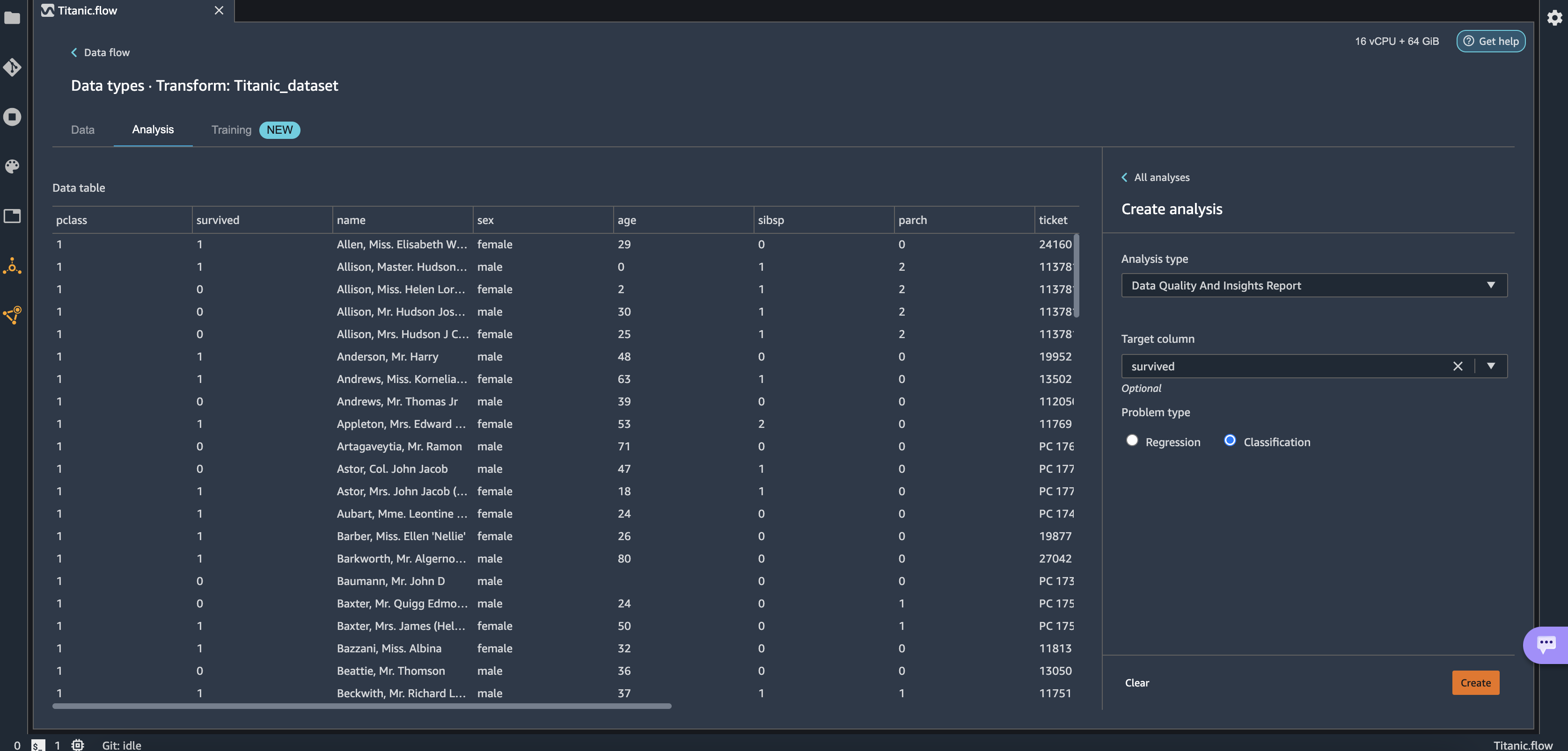
2. Choose Get data insights.
   
   This opens the Analysis tab on the data, in which you can create a Data Quality and Insights Report. When you create this report, Data Wrangler gives you the option to select a target column. A target column is a column that you’re trying to predict. When you choose a target column, Data Wrangler automatically creates a target column analysis. It also ranks the features in the order of their predictive power. When you select a target column, you must specify whether you’re trying to solve a regression or a classification problem.
3. Choose the column survived as the target column because that’s the value we want to predict.
4. For Problem type¸ select Classification¸ because we want to know whether a passenger belongs to the survived or not survived classes.
5. Choose Create.
   This creates an analysis on your dataset that contains relevant points like a summary of the dataset, duplicate rows, anomalous samples, feature details, and more. To learn more about the Data Quality and Insights Report, refer to Accelerate data preparation with data quality and insights in Amazon SageMaker Data Wrangler and Get Insights On Data and Data Quality.
   Let’s get a quick look at the dataset itself.
6. Choose the Data tab to visualize the data as a table.Let’s now generate some example data visualizations.
7. Choose the Analysis tab to start visualizing your data. You can generate three histograms: the first two visualize the number of people that survived based on the sex and class columns, as shown in the following screenshots.The third visualizes the ages of the people that boarded the Titanic.Let’s perform some transformations on the data,
8. First, drop the columns ticket, cabin, and name.
9. Next, perform one-hot encoding on the categorical columns embarked and sex, and home.dest.
10. Finally, fill in missing values for the columns boat and body with a 0 value.
    Your dataset now looks something like the following screenshot.
11. Now split the dataset into three sets: a training set with 70% of the data, a validation set with 20% of the data, and a test set with 10% of the data.The splits done here use the stratified split approach using the survived variable and are just for the sake of the demonstration.Now let’s configure the destination of our data.
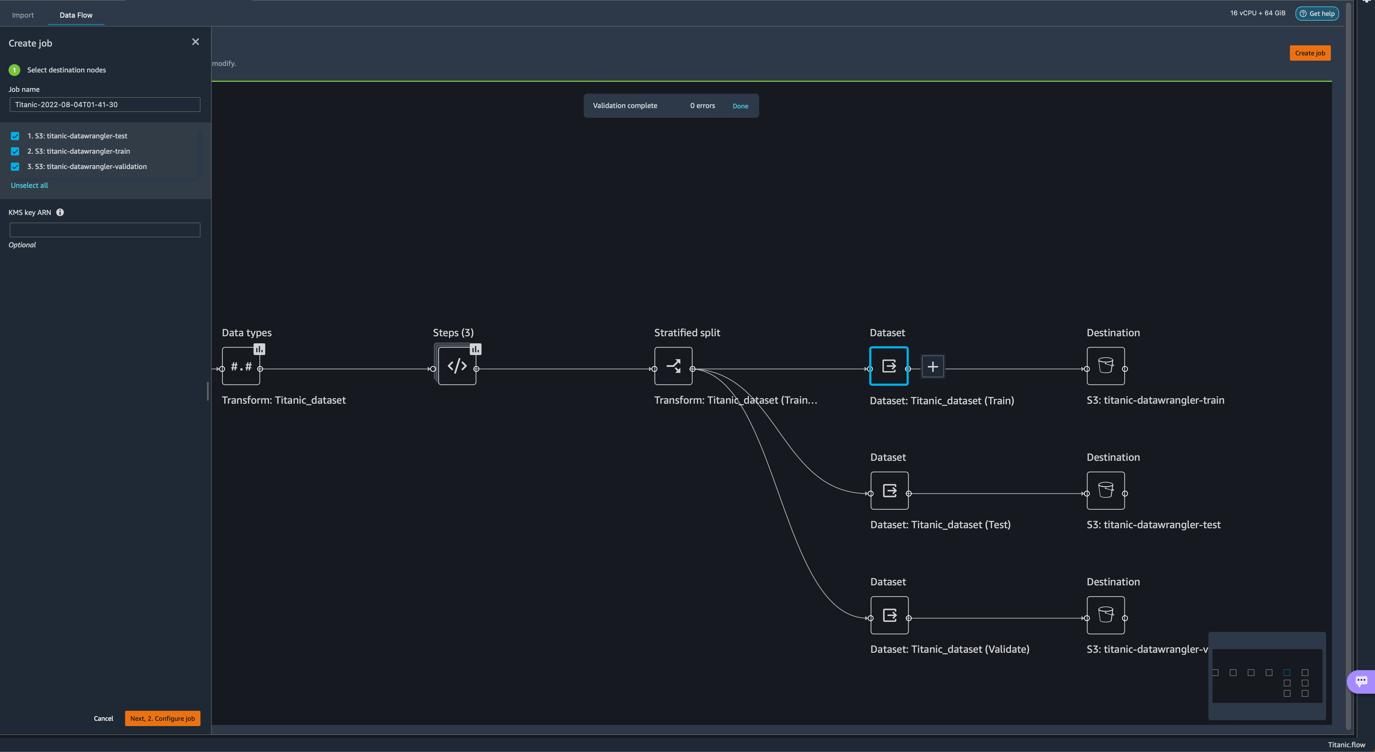
12. Choose the plus sign on each Dataset node, choose Add destination, and choose S3 to add an Amazon S3 destination for the transformed datasets.
13. In the Add a destination pane, you can configure the Amazon S3 details to store your processed datasets.Our Titanic flow should now look like the following screenshot.You can now transform all the data using SageMaker processing jobs.
14. Choose Create job.
15. Keep the default values and choose Next.
16. Choose Run.A new SageMaker processing job is now created. You can see the job’s details and track its progress on the SageMaker console under Processing jobs.When the processing job is complete, you can navigate to any of the S3 locations specified for storing the datasets and query the data just to confirm that the processing was successful. You can now use this data to feed your ML projects.

Launch an Autopilot experiment to create a classifier

You can now launch Autopilot experiments directly from Data Wrangler and use the data at any of the steps in the flow to automatically train a model on the data.

1. Choose the Dataset node called Titanic_dataset (train) and navigate to the Train tab.
   Before training, you need to first export your data to Amazon S3.
2. Follow the instructions to export your data to an S3 location of your choice.
   You can specify to export the data in CSV or Parquet format for increased efficiency. Additionally, you can specify an AWS Key Management Service (AWS KMS) key to encrypt your data.
   On the next page, you configure your Autopilot experiment.
3. Unless your data is split into several parts, leave the default value under Connect your data.
4. For this demonstration, leave the default values for Experiment name and Output data location.
5. Under Advanced settings, expand Machine learning problem type.
6. Choose Binary classification as the problem type and Accuracy as the objective metric.You specify these two values manually even though Autopilot is capable of inferring them from the data.
7. Leave the rest of the fields with the default values and choose Create Experiment.Wait for a couple of minutes until the Autopilot experiment is complete, and you will see a leaderboard like the following with each of the models obtained by Autopilot.

You can now choose to deploy any of the models in the leaderboard for inference.

Clean up

When you’re not using Data Wrangler, it’s important to shut down the instance on which it runs to avoid incurring additional fees.

To avoid losing work, save your data flow before shutting Data Wrangler down.

1. To save your data flow in Amazon SageMaker Studio, choose File, then choose Save Data Wrangler Flow.
   Data Wrangler automatically saves your data flow every 60 seconds.
2. To shut down the Data Wrangler instance, in Studio, choose Running Instances and Kernels.
3. Under RUNNING APPS, choose the shutdown icon next to the sagemaker-data-wrangler-1.0 app.
4. Choose Shut down all to confirm.Data Wrangler runs on an ml.m5.4xlarge instance. This instance disappears from RUNNING INSTANCES when you shut down the Data Wrangler app.

After you shut down the Data Wrangler app, it has to restart the next time you open a Data Wrangler flow file. This can take a few minutes.

Conclusion

In this post, we demonstrated how you can use the new sample dataset on Data Wrangler to explore Data Wrangler’s features without needing to bring your own data. We also presented two additional features: the loading page to let you visually track the progress of the data being imported into Data Wrangler, and product suggestions that provide useful tips to get started with Data Wrangler. We went further to show how you can create SageMaker processing jobs and launch Autopilot experiments directly from the Data Wrangler user interface.

To learn more about using data flows with Data Wrangler, refer to Create and Use a Data Wrangler Flow and Amazon SageMaker Pricing. To get started with Data Wrangler, see Prepare ML Data with Amazon SageMaker Data Wrangler. To learn more about Autopilot and AutoML on SageMaker, visit Automate model development with Amazon SageMaker Autopilot.

About the authors

David Laredo is a Prototyping Architect at AWS Envision Engineering in LATAM, where he has helped develop multiple machine learning prototypes. Previously, he worked as a Machine Learning Engineer and has been doing machine learning for over 5 years. His areas of interest are NLP, time series, and end-to-end ML.

Parth Patel is a Solutions Architect at AWS in the San Francisco Bay Area. Parth guides customers to accelerate their journey to the cloud and helps them adopt the AWS Cloud successfully. He focuses on ML and application modernization.

Read More