Reverse engineering the NTK: towards first-principles architecture design


Foundational works showed how to find the kernel corresponding to a wide network. We find the inverse mapping, showing how to find the wide network corresponding to a given kernel.

Deep neural networks have enabled technological wonders ranging from voice recognition to machine transition to protein engineering, but their design and application is nonetheless notoriously unprincipled.
The development of tools and methods to guide this process is one of the grand challenges of deep learning theory.
In Reverse Engineering the Neural Tangent Kernel, we propose a paradigm for bringing some principle to the art of architecture design using recent theoretical breakthroughs: first design a good kernel function – often a much easier task – and then “reverse-engineer” a net-kernel equivalence to translate the chosen kernel into a neural network.
Our main theoretical result enables the design of activation functions from first principles, and we use it to create one activation function that mimics deep (textrm{ReLU}) network performance with just one hidden layer and another that soundly outperforms deep (textrm{ReLU}) networks on a synthetic task.

Fast Beam Search Decoding in PyTorch with TorchAudio and Flashlight Text

Beam search decoding with industry-leading speed from Flashlight Text (part of the Flashlight ML framework) is now available with official support in TorchAudio, bringing high-performance beam search and text utilities for speech and text applications built on top of PyTorch. The current integration supports CTC-style decoding, but it can be used for any modeling setting that outputs token-level probability distributions over time steps.

A brief beam search refresher

In speech and language settings, beam search is an efficient, greedy algorithm that can convert sequences of continuous values (i.e. probabilities or scores) into graphs or sequences (i.e. tokens, word-pieces, words) using optional constraints on valid sequences (i.e. a lexicon), optional external scoring (i.e. an LM which scores valid sequences), and other score adjustments for particular sequences.

In the example that follows, we’ll consider — a token set of {ϵ, a, b}, where ϵ is a special token that we can imagine denotes a space between words or a pause in speech. Graphics here and below are taken from Awni Hannun’s excellent distill.pub writeup on CTC and beam search.

With a greedy-like approach, beam search considers the next viable token given an existing sequence of tokens — in the example above, a, b, b is a valid sequence, but a, b, a is not. We rank each possible next token at each step of the beam search according to a scoring function. Scoring functions (s) typically looks something like:

Where ŷ is a potential path/sequence of tokens, x is the input (P(ŷ|x) represents the model’s predictions over time), and 𝛼 is a weight on the language model probability (P(y) the probability of the sequence under the language model). Some scoring functions add 𝜷 which adjusts a score based on the length of the predicted sequence |ŷ|. This particular scoring function is used in FAIR’s prior work on end-to-end ASR, and there are many variations on scoring functions which can vary across application areas.

Given a particular sequence, to assess the next viable token in that sequence (perhaps constrained by a set of allowed words or sequences, such as a lexicon of words), the beam search algorithm scores the sequence with each candidate token added, and sorts token candidates based on those scores. For efficiency and since the number of paths is exponential in the token set size, the top-k highest-scoring candidates are kept — k represents the beam size.

There are many other nuances with how beam search can progress: similar hypothesis sequences can be “merged”, for instance.

The scoring function can be further augmented to up/down-weight token insertion or long or short words. Scoring with stronger external language models, while incurring computational cost, can also significantly improve performance; this is frequently referred to as LM fusion. There are many other knobs to tune for decoding — these are documented in TorchAudio’s documentation and explored further in TorchAudio’s ASR Inference tutorial. Since decoding is quite efficient, parameters can be easily swept and tuned.

Beam search has been used in ASR extensively over the years in far too many works to cite, and in strong, recent results and systems including wav2vec 2.0 and NVIDIA’s NeMo.

Why beam search?

Beam search remains a fast competitor to heavier-weight decoding approaches such as RNN-Transducer that Google has invested in putting on-device and has shown strong results with on common benchmarks. Autoregressive text models at scale can benefit from beam search as well. Among other things, beam search gives:

  • A flexible performance/latency tradeoff — by adjusting beam size and the external LM, users can sacrifice latency for accuracy or pay for more accurate results with a small latency cost. Decoding with no external LM can improve results at very little performance cost.
  • Portability without retraining — existing neural models can benefit from multiple decoding setups and plug-and-play with external LMs without training or fine-tuning.
  • A compelling complexity/accuracy tradeoff — adding beam search to an existing modeling pipeline incurs little additional complexity and can improve performance.

Performance Benchmarks

Today’s most commonly-used beam search decoding libraries today that support external language model integration include Kensho’s pyctcdecode, NVIDIA’s NeMo toolkit. We benchmark the TorchAudio + Flashlight decoder against them with a wav2vec 2.0 base model trained on 100 hours of audio evaluated on LibriSpeech dev-other with the official KenLM 3-gram LM. Benchmarks were run on Intel E5-2698 CPUs on a single thread. All computation was in-memory — KenLM memory mapping was disabled as it wasn’t widely supported.

When benchmarking, we measure the time-to-WER (word error rate) — because of subtle differences in the implementation of decoding algorithms and the complex relationships between parameters and decoding speed, some hyperparameters differed across runs. To fairly assess performance, we first sweep for parameters that achieve a baseline WER, minimizing beam size if possible.

Decoding performance on Librispeech dev-other of a pretrained wav2vec 2.0 model. TorchAudio + Flashlight decoding outperforms by an order of magnitude at low WERs.

Time-to-WER results, deferring to smaller beam size, across decoders. The TorchAudio + Flashlight decoder scales far better with larger beam sizes and at lower WERs.

TorchAudio API and Usage

TorchAudio provides a Python API for CTC beam search decoding, with support for the following:

  • lexicon and lexicon-free decoding
  • KenLM n-gram language model integration
  • character and word-piece decoding
  • sample pretrained LibriSpeech KenLM models and corresponding lexicon and token files
  • various customizable beam search parameters (beam size, pruning threshold, LM weight…)

To set up the decoder, use the factory function torchaudio.models.decoder.ctc_decoder

from torchaudio.models.decoder import ctc_decoder, download_pretrained_files
files = download_pretrained_files("librispeech-4-gram")
decoder = ctc_decoder(
   lexicon=files.lexicon,
   tokens=files.tokens,
   lm=files.lm,
   nbest=1,
   ... additional optional customizable args ...
)

Given emissions of shape (batch, time, num_tokens), the decoder will compute and return a List of batch Lists, each consisting of the nbest hypotheses corresponding to the emissions. Each hypothesis can be further broken down into tokens, words (if a lexicon is provided), score, and timesteps components.

emissions = acoustic_model(waveforms)  # (B, T, N)
batch_hypotheses = decoder(emissions)  # List[List[CTCHypothesis]]

# transcript for a lexicon decoder
transcripts = [" ".join(hypo[0].words) for hypo in batch_hypotheses]

# transcript for a lexicon free decoder, splitting by sil token
batch_tokens = [decoder.idxs_to_tokens(hypo[0].tokens) for hypo in batch_hypotheses]
transcripts = ["".join(tokens) for tokens in batch_tokens]

Please refer to the documentation for more API details, and the tutorial (ASR Inference Decoding) or sample inference script for more usage examples.

Upcoming Improvements

Full NNLM support — decoding with large neural language models (e.g. transformers) remains somewhat unexplored at scale. Already supported in Flashlight, we plan to add support in TorchAudio, allowing users to use custom decoder-compatible LMs. Custom word level language models are already available in the nightly TorchAudio build, and is slated to be released in TorchAudio 0.13.

Autoregressive/seq2seq decoding — Flashlight Text also supports sequence-to-sequence (seq2seq) decoding for autoregressive models, which we hope to add bindings for and add to TorchAudio and TorchText with efficient GPU implementations as well.

Better build support — to benefit from improvements in Flashlight Text, TorchAudio will directly submodule Flashlight Text to make upstreaming modifications and improvements easier. This is already in effect in the nightly TorchAudio build, and is slated to be released in TorchAudio 0.13.

Citation

To cite the decoder, please use the following:

@inproceedings{kahn2022flashlight,
  title={Flashlight: Enabling innovation in tools for machine learning},
  author={Kahn, Jacob D and Pratap, Vineel and Likhomanenko, Tatiana and Xu, Qiantong and Hannun, Awni and Cai, Jeff and Tomasello, Paden and Lee, Ann and Grave, Edouard and Avidov, Gilad and others},
  booktitle={International Conference on Machine Learning},
  pages={10557--10574},
  year={2022},
  organization={PMLR}
}
@inproceedings{yang2022torchaudio,
  title={Torchaudio: Building blocks for audio and speech processing},
  author={Yang, Yao-Yuan and Hira, Moto and Ni, Zhaoheng and Astafurov, Artyom and Chen, Caroline and Puhrsch, Christian and Pollack, David and Genzel, Dmitriy and Greenberg, Donny and Yang, Edward Z and others},
  booktitle={ICASSP 2022-2022 IEEE International Conference on Acoustics, Speech and Signal Processing (ICASSP)},
  pages={6982--6986},
  year={2022},
  organization={IEEE}
}

Read More

Run image segmentation with Amazon SageMaker JumpStart

In December 2020, AWS announced the general availability of Amazon SageMaker JumpStart, a capability of Amazon SageMaker that helps you quickly and easily get started with machine learning (ML). JumpStart provides one-click fine-tuning and deployment of a wide variety of pre-trained models across popular ML tasks, as well as a selection of end-to-end solutions that solve common business problems. These features remove the heavy lifting from each step of the ML process, making it easier to develop high-quality models and reducing time to deployment.

This post is the third in a series on using JumpStart for specific ML tasks. In the first post, we showed how you can run image classification use cases on JumpStart. In the second post, we showed how you can run text classification use cases on JumpStart. In this post, we provide a step-by-step walkthrough on how to fine-tune and deploy an image segmentation model, using trained models from MXNet. We explore two ways of obtaining the same result: via JumpStart’s graphical interface on Amazon SageMaker Studio, and programmatically through JumpStart APIs.

If you want to jump straight into the JumpStart API code we explain in this post, you can refer to the following sample Jupyter notebooks:

JumpStart overview

JumpStart helps you get started with ML models for a variety of tasks without writing a single line of code. At the time of writing, JumpStart enables you to do the following:

  • Deploy pre-trained models for common ML tasks – JumpStart enables you to address common ML tasks with no development effort by providing easy deployment of models pre-trained on large, publicly available datasets. The ML research community has put a large amount of effort into making a majority of recently developed models publicly available for use. JumpStart hosts a collection of over 300 models, spanning the 15 most popular ML tasks such as object detection, text classification, and text generation, making it easy for beginners to use them. These models are drawn from popular model hubs such as TensorFlow, PyTorch, Hugging Face, and MXNet.
  • Fine-tune pre-trained models – JumpStart allows you to fine-tune pre-trained models with no need to write your own training algorithm. In ML, the ability to transfer the knowledge learned in one domain to another domain is called transfer learning. You can use transfer learning to produce accurate models on your smaller datasets, with much lower training costs than the ones involved in training the original model. JumpStart also includes popular training algorithms based on LightGBM, CatBoost, XGBoost, and Scikit-learn, which you can train from scratch for tabular regression and classification.
  • Use pre-built solutions – JumpStart provides a set of 17 solutions for common ML use cases, such as demand forecasting and industrial and financial applications, which you can deploy with just a few clicks. Solutions are end-to-end ML applications that string together various AWS services to solve a particular business use case. They use AWS CloudFormation templates and reference architectures for quick deployment, which means they’re fully customizable.
  • Refer to notebook examples for SageMaker algorithms – SageMaker provides a suite of built-in algorithms to help data scientists and ML practitioners get started with training and deploying ML models quickly. JumpStart provides sample notebooks that you can use to quickly use these algorithms.
  • Review training videos and blogs – JumpStart also provides numerous blog posts and videos that teach you how to use different functionalities within SageMaker.

JumpStart accepts custom VPC settings and AWS Key Management Service (AWS KMS) encryption keys, so you can use the available models and solutions securely within your enterprise environment. You can pass your security settings to JumpStart within Studio or through the SageMaker Python SDK.

Semantic segmentation

Semantic segmentation delineates each class of objects appearing in an input image. It tags (classifies) each pixel of the input image with a class label from a predefined set of classes. Multiple objects of the same class are mapped to the same mask.

The model available for fine-tuning builds a fully convolutional network (FCN) “head” on top of the base network. The fine-tuning step fine-tunes the FCNHead while keeping the parameters of the rest of the model frozen, and returns the fine-tuned model. The objective is to minimize per-pixel softmax cross entropy loss to train the FCN. The model returned by fine-tuning can be further deployed for inference.

The input directory should look like the following code if the training data contains two images. The names of the .png files can be anything.

input_directory
    |--images
        |--abc.png
        |--def.png
    |--masks
        |--abc.png
        |--def.png
    class_label_to_prediction_index.json

The mask files should have class label information for each pixel.

Instance segmentation

Instance segmentation detects and delineates each distinct object of interest appearing in an image. It tags every pixel with an instance label. Whereas semantic segmentation assigns the same tag to pixels of multiple objects of the same class, instance segmentation further labels pixels corresponding to each occurrence of an object on the image with a separate tag.

Currently, JumpStart offers inference-only models for instance segmentation and doesn’t support fine-tuning.

The following images illustrate the difference between the inference in semantic segmentation and instance segmentation. The original image has two people in the image. Semantic segmentation treats multiple people in the image as one entity: Person. However, instance segmentation identifies individual people within the Person category.

Solution overview

The following sections provide a step-by-step demo to perform semantic segmentation with JumpStart, both via the Studio UI and via JumpStart APIs.

We walk through the following steps:

  1. Access JumpStart through the Studio UI:
    1. Run inference on the pre-trained model.
    2. Fine-tune the pre-trained model.
  2. Use JumpStart programmatically with the SageMaker Python SDK:
    1. Run inference on the pre-trained model.
    2. Fine-tune the pre-trained model.

We also discuss additional advanced features of JumpStart.

Access JumpStart through the Studio UI

In this section, we demonstrate how to train and deploy JumpStart models through the Studio UI.

Run inference on the pre-trained model

The following video shows you how to find a pre-trained semantic segmentation model on JumpStart and deploy it. The model page contains valuable information about the model, how to use it, expected data format, and some fine-tuning details. You can deploy any of the pre-trained models available in JumpStart. For inference, we pick the ml.g4dn.xlarge instance type. It provides the GPU acceleration needed for low inference latency, but at a lower price point. After you configure the SageMaker hosting instance, choose Deploy. It may take 5–10 minutes until your persistent endpoint is up and running.

After a few minutes, your endpoint is operational and ready to respond to inference requests.

Similarly, you can deploy a pre-trained instance segmentation model by following the same steps in the preceding video while searching for instance segmentation instead of semantic segmentation in the JumpStart search bar.

Fine-tune the pre-trained model

The following video shows how to find and fine-tune a semantic segmentation model in JumpStart. In the video, we fine-tune the model using the PennFudanPed dataset, provided by default in JumpStart, which you can download under the Apache 2.0 License.

Fine-tuning on your own dataset involves taking the correct formatting of data (as explained on the model page), uploading it to Amazon Simple Storage Service (Amazon S3), and specifying its location in the data source configuration. We use the same hyperparameter values set by default (number of epochs, learning rate, and batch size). We also use a GPU-backed ml.p3.2xlarge as our SageMaker training instance.

You can monitor your training job running directly on the Studio console, and are notified upon its completion. After training is complete, you can deploy the fine-tuned model from the same page that holds the training job details. The deployment workflow is the same as deploying a pre-trained model.

Use JumpStart programmatically with the SageMaker SDK

In the preceding sections, we showed how you can use the JumpStart UI to deploy a pre-trained model and fine-tune it interactively, in a matter of a few clicks. However, you can also use JumpStart’s models and easy fine-tuning programmatically by using APIs that are integrated into the SageMaker SDK. We now go over a quick example of how you can replicate the preceding process. All the steps in this demo are available in the accompanying notebooks Introduction to JumpStart – Instance Segmentation and Introduction to JumpStart – Semantic Segmentation.

Run inference on the pre-trained model

In this section, we choose an appropriate pre-trained model in JumpStart, deploy this model to a SageMaker endpoint, and run inference on the deployed endpoint.

SageMaker is a platform based on Docker containers. JumpStart uses the available framework-specific SageMaker Deep Learning Containers (DLCs). We fetch any additional packages, as well as scripts to handle training and inference for the selected task. Finally, the pre-trained model artifacts are separately fetched with model_uris, which provides flexibility to the platform. You can use any number of models pre-trained for the same task with a single training or inference script. See the following code:

model_id, model_version = "mxnet-semseg-fcn-resnet50-ade", "*"

# Retrieve the inference docker container uri
deploy_image_uri = image_uris.retrieve(
    region=None,
    framework=None,  # automatically inferred from model_id
    image_scope="inference",
    model_id=model_id,
    model_version=model_version,
    instance_type=inference_instance_type,
)

# Retrieve the inference script uri
deploy_source_uri = script_uris.retrieve(model_id=model_id, model_version=model_version, script_scope="inference")

base_model_uri = model_uris.retrieve(model_id=model_id, model_version=model_version, model_scope="inference")

For instance segmentation, we can set model_id to mxnet-semseg-fcn-resnet50-ade. The is in the identifier corresponds to instance segmentation.

Next, we feed the resources into a SageMaker model instance and deploy an endpoint:

# Create the SageMaker model instance
model = Model(
    image_uri=deploy_image_uri,
    source_dir=deploy_source_uri,
    model_data=base_model_uri,
    entry_point="inference.py",  # entry point file in source_dir and present in deploy_source_uri
    role=aws_role,
    predictor_cls=Predictor,
    name=endpoint_name,
)

# deploy the Model. Note that we need to pass Predictor class when we deploy model through Model class,
# for being able to run inference through the sagemaker API.
base_model_predictor = model.deploy(
    initial_instance_count=1,
    instance_type=inference_instance_type,
    predictor_cls=Predictor,
    endpoint_name=endpoint_name,
)

After a few minutes, our model is deployed and we can get predictions from it in real time!

The following code snippet gives you a glimpse of what semantic segmentation looks like. The predicted mask for each pixel is visualized. To get inferences from a deployed model, an input image needs to be supplied in binary format. The response of the endpoint is a predicted label for each pixel in the image. We use the query_endpoint and parse_response helper functions, which are defined in the accompanying notebook:

query_response = query(base_model_predictor, pedestrian_img)
predictions, labels, image_labels = parse_response(query_response)
print("Objects present in the picture:", image_labels)

Fine-tune the pre-trained model

To fine-tune a selected model, we need to get that model’s URI, as well as that of the training script and the container image used for training. Thankfully, these three inputs depend solely on the model name, version (for a list of the available models, see JumpStart Available Model Table), and the type of instance you want to train on. This is demonstrated in the following code snippet:

from sagemaker import image_uris, model_uris, script_uris

model_id, model_version = "mxnet-semseg-fcn-resnet50-ade", "*"
training_instance_type = "ml.p3.2xlarge"
train_image_uri = image_uris.retrieve(
    region=None,
    framework=None,
    model_id=model_id,
    model_version=model_version,
    image_scope="training",
    instance_type=training_instance_type,)# Retrieve the training script

train_source_uri = script_uris.retrieve(model_id=model_id, model_version=model_version, script_scope="training")# Retrieve the pre-trained model tarball to further fine-tune

train_model_uri = model_uris.retrieve(model_id=model_id, model_version=model_version, model_scope="training")

We retrieve the model_id corresponding to the same model we used previously. You can now fine-tune this JumpStart model on your own custom dataset using the SageMaker SDK. We use a dataset that is publicly hosted on Amazon S3, conveniently focused on semantic segmentation. The dataset should be structured for fine-tuning as explained in the previous section. See the following example code:

# URI of your training dataset
training_data_bucket = f"jumpstart-cache-prod-{aws_region}"
training_data_prefix = "training-datasets/PennFudanPed_SemSeg/"
training_dataset_s3_path = f"s3://{training_data_bucket}/{training_data_prefix}"
training_job_name = name_from_base(f"jumpstart-example-{model_id}-transfer-learning")# Create SageMaker Estimator instance
semseg_estimator = Estimator(
    role=aws_role,
    image_uri=train_image_uri,
    source_dir=train_source_uri,
    model_uri=train_model_uri,
    entry_point="transfer_learning.py",
    instance_count=1,
    instance_type=training_instance_type,
    max_run=360000,
    hyperparameters=hyperparameters,
    output_path=s3_output_location,)# Launch a SageMaker Training job by passing s3 path of the training data
semseg_estimator.fit({"training": training_dataset_s3_path}, logs=True)

We obtain the same default hyperparameters for our selected model as the ones we saw in the previous section, using sagemaker.hyperparameters.retrieve_default(). We then instantiate a SageMaker estimator and call the .fit method to start fine-tuning our model, passing it the Amazon S3 URI for our training data. The entry_point script provided is named transfer_learning.py (the same for other tasks and models), and the input data channel passed to .fit must be named training.

While the algorithm trains, you can monitor its progress either in the SageMaker notebook where you’re running the code itself, or on Amazon CloudWatch. When training is complete, the fine-tuned model artifacts are uploaded to the Amazon S3 output location specified in the training configuration. You can now deploy the model in the same manner as the pre-trained model.

Advanced features

In addition to fine-tuning and deploying pre-trained models, JumpStart offers many advanced features.

The first is automatic model tuning. This allows you to automatically tune your ML models to find the hyperparameter values with the highest accuracy within the range provided through the SageMaker API.

The second is incremental training. This allows you to train a model you have already fine-tuned using an expanded dataset that contains an underlying pattern not accounted for in previous fine-tuning runs, which resulted in poor model performance. Incremental training saves both time and resources because you don’t need to retrain the model from scratch.

Conclusion

In this post, we showed how to fine-tune and deploy a pre-trained semantic segmentation model, and how to adapt it for instance segmentation using JumpStart. You can accomplish this without needing to write code. Try out the solution on your own and send us your comments.

To learn more about JumpStart and how you can use open-source pre-trained models for a variety of other ML tasks, check out the following AWS re:Invent 2020 video.


About the Authors

Dr. Vivek Madan is an Applied Scientist with the Amazon SageMaker JumpStart team. He got his PhD from University of Illinois at Urbana-Champaign and was a Post Doctoral Researcher at Georgia Tech. He is an active researcher in machine learning and algorithm design and has published papers in EMNLP, ICLR, COLT, FOCS, and SODA conferences.

Santosh Kulkarni is an Enterprise Solutions Architect at Amazon Web Services who works with sports customers in Australia. He is passionate about building large-scale distributed applications to solve business problems using his knowledge in AI/ML, big data, and software development.

Leonardo Bachega is a senior scientist and manager in the Amazon SageMaker JumpStart team. He’s passionate about building AI services for computer vision.

Read More

Recurrent Model-Free RL Can Be a Strong Baseline for Many POMDPs

Figure 1. Our implementation of recurrent model-free RL outperforms the on-policy version (PPO/A2C-GRU), and a recent model-based POMDP algorithm (VRM) on most tasks of a POMDP benchmark where VRM was evaluated in their paper.

While algorithms for decision-making typically focus on relatively easy problems where everything is known, most realistic problems involve noise and incomplete information. Complex algorithms have been proposed to tackle these complex problems, but there’s a simple approach that (in theory) works on both the easy and the complex problems. We show how to make this simple approach work in practice.

Why POMDPs?

Decision-making tasks in the real world are messy, with noise, occlusions, and uncertainty that are typically missing from their canonical problem formulation as a Markov decision process (MDP; Bellman, 1957). In contrast, Partially Observable MDPs (POMDPs; Åström, 1965) can capture the uncertainty in the states, rewards, and dynamics. Such uncertainty arises in applications such as robotics, healthcare, NLP and finance.

Apart from being realistic, POMDPs are a general framework that contains many subareas in RL, including:

What is recurrent model-free RL?

Solving POMDPs is hard because the agent needs to learn two tasks simultaneously: inference and control. Inference aims to infer the posterior over current states conditioned on history. Control aims to perform RL / planning algorithms on the inferred state space. While prior methods typically decouple the two jobs with separate models, deep learning, provides us with a general and simple baseline: combine an off-the-shelf RL algorithm with a recurrent neural network (RNN; e.g., LSTM (Hochreiter & Schmidhuber, 1997) and GRU (Chung et al., 2014)).

By backpropagating the gradients from policy loss, RNNs make it possible to process sequences (histories in POMDPs) and learn implicit inference on the state space for control. We refer to it as recurrent model-free RL. Fig. 2 presents our design, where actor and critic networks each have an RNN as the history encoder.

Figure 2. Our recurrent actor and critic architecture. Each network contains an RNN as the sequence encoder. The recurrent actor takes as input current observation, previous action and reward (optional), and outputs current action. The recurrent critic also takes current action as an input and outputs Q-values.

Recurrent model-free RL has many merits at first glance:

  • Conceptually simple. The policy purely learns from rewards, without extra objectives.
  • Easy to implement. Practitioners can just change several lines of code from model-free RL.
  • Expressive in theory. RNNs have been shown as universal function approximators (Siegelmann & Sontag, 1995, Schäfer & Zimmermann, 2006) and, thus recurrent model-free RL can (approximately) express any memory-based policies.

Due to its simplicity and expressivity, there is rich literature (Schmidhuber, 1991, Bakker, 2001, Wierstra et al., 2007, Heess et al., 2015, Hausknecht & Stone, 2015) on studying different RL algorithms and RNN architectures of recurrent model-free RL. However, prior work has shown that it often fails in practice with poor or unstable performance (Igl et al., 2018, Hung et al., 2018, Packer et al., 2018, Rakelly et al., 2019, Zintgraf et al., 2020, Han et al., 2020, Zhang et al., 2021, Raposo et al., 2021), with only a few exceptions (Yu et al., 2019, Fakoor et al., 2020).

Motivated by the poor performance of this simple baseline, prior work has proposed more sophisticated methods. Some introduce model-based objectives that explicitly learn inference, while others incorporate the assumptions used in the subarea of POMDPs as inductive bias. Both achieve good results on a range of respective tasks, although the model-based methods may have staleness issue in the belief states stored in the replay buffer, and the specialized methods require more assumptions than recurrent model-free RL (e.g., meta-RL methods normally assumes the hidden variable is constant within a single episode).

How to train recurrent model-free RL?

In this work, we found that recurrent model-Free RL is not fatally failed, but just needed to be implemented differently, with differences including:

  1. Separating the RNNs in actor and critic networks. Un-sharing the weights can prevent gradient explosion, and can be the difference between the algorithm learning nothing and solving the task almost perfectly.
  2. Using an off-policy RL algorithm to improve sample efficiency. Using, say, TD3 instead of PPO greatly improves sample efficiency.
  3. Tuning the RNN context length. We found that the RNN architectures (LSTM and GRU) do not matter much, but the RNN context length (the length of the sequence fed into the RL algorithm), is crucial and depends on the task. We suggest choosing a medium length as a start.

Properly tuned, the simple baseline outperforms alternatives on many POMDPs

With these changes, our implementation of recurrent model-free RL is at least on par with (if not much better than) prior methods, on the tasks those prior methods were designed to solve. While prior methods are typically designed to solve special cases of POMDPs, recurrent model-free RL applies to all types of POMDPs.

Our first comparison looks at meta-RL tasks, which are usually approached by methods that decouple the task inference and reward maximization steps (Rakelly et al., 2019, Zintgraf et al., 2020). When comparing these prototypical methods (on-policy variBAD (Zintgraf et al., 2020) and off-policy variBAD (Dorfman et al., 2020)), we find that our recurrent model-free approach can often perform at least on par with them. These results (Fig. 3, 4) suggest that disentangling inference and control may be not that necessary in many tasks.

Figure 3. Two meta-RL environments from off-policy variBAD (left: Semi-Circle, right: Wind), where ours outperforms off-policy variBAD.
Figure 4. Two meta-RL environments from on-policy variBAD (left: Cheetah-Dir, right: Ant-Dir), where we have mixed results.

Next, we move on to the robust RL setting, which is mostly solved by algorithms that explicitly maximize the worst returns (Rajeswaran et al., 2017, Mankowitz et al., 2020). By comparing one recent robust RL algorithm (Jiang et al., 2021), we find that our recurrent model-free approach performs better in all the tasks. The results (Fig. 5) indicate that with the power of implicit task inference with RNNs, we can improve both average and worst returns.

Figure 5. One robust RL environment from MRPO, Cheetah-Robust (left: average return; right: worst return), where ours outperforms MRPO.

Then we explore the generalization in RL, where people have different kinds of specialized methods, including policy regularization (Farebrother et al., 2018) and data augmentation (Lee et al., 2020). Here we choose a popular benchmark SunBlaze (Packer et al., 2018) which provides a specialized baseline EPOpt-PPO-FF (Rajeswaran et al., 2017). The results (Fig. 6) show that despite not explicitly enhancing generalization, our recurrent model-free approach can perform better in extrapolation than the baseline. This suggests that the task inference learned by RNN is generalizable.

Figure 6. One generalization in RL environment from SunBlaze, Hopper-Generalize (left: interpolated success rate; right: extrapolated success rate), where ours outperforms EPOpt-PPO-FF on extrapolation.

Finally, we study the temporal credit assignment domain where the methods for solving it usually involve reward decomposition/redistribution (Liu et al., 2019, Hung et al., 2018). Here, we choose a recent specialized method IMPALA+SR (Raposo et al., 2021), and evaluate our method on their benchmark with pixel-based discrete control and sparse rewards. Despite being unaware of the reward structure and not performing credit assignment explicitly, our recurrent model-free approach can perform better. The results (Fig. 7) indicate that recurrent policies can effectively cope with sparse rewards, perhaps better than previously expected.

Figure 7. Two temporal credit assignment environments from IMPALA+SR (left: Delayed-Catch, right: Key-to-Door), where ours outperforms IMPALA+SR.

Conclusion

In a sense, our finding can be interpreted as echoing the motivation for deep learning: we can achieve better results by reducing a method to a single differentiable architecture, optimized end-to-end with a single loss. This is exciting because RL systems often involve many interconnected parts (e.g., feature extracting, model learning, value estimation) trained with different objectives, but perhaps they might be replaced by end-to-end approaches if equipped with sufficiently expressive architectures.

We have open-sourced the code on GitHub to support reproducibility and to help future work develop better POMDP algorithms. Please see our project site for the paper and our ICML 2022 presentation.

Read More

Process mortgage documents with intelligent document processing using Amazon Textract and Amazon Comprehend

Organizations in the lending and mortgage industry process thousands of documents on a daily basis. From a new mortgage application to mortgage refinance, these business processes involve hundreds of documents per application. There is limited automation available today to process and extract information from all the documents, especially due to varying formats and layouts. Due to high volume of applications, capturing strategic insights and getting key information from the contents is a time-consuming, highly manual, error prone and expensive process. Legacy optical character recognition (OCR) tools are cost-prohibitive, error-prone, involve a lot of configuring, and are difficult to scale. Intelligent document processing (IDP) with AWS artificial intelligence (AI) services helps automate and accelerate the mortgage application processing with goals of faster and quality decisions, while reducing overall costs.

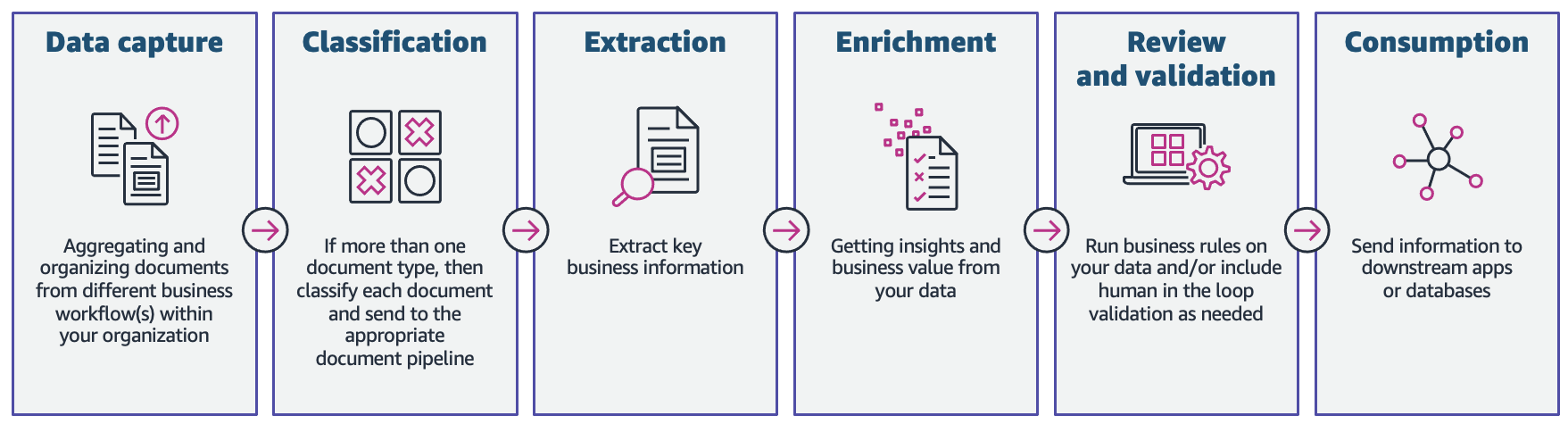
In this post, we demonstrate how you can utilize machine learning (ML) capabilities with Amazon Textract, and Amazon Comprehend to process documents in a new mortgage application, without the need for ML skills. We explore the various phases of IDP as shown in the following figure, and how they connect to the steps involved in a mortgage application process, such as application submission, underwriting, verification, and closing.

Image shows the phases of intelligent document processing (IDP).

Although each mortgage application may be unique, we took into account some of the most common documents that are included in a mortgage application, such as the Unified Residential Loan Application (URLA-1003) form, 1099 forms, and mortgage note.

Solution overview

Amazon Textract is an ML service that automatically extracts text, handwriting, and data from scanned documents using pre-trained ML models. Amazon Comprehend is a natural-language processing (NLP) service that uses ML to uncover valuable insights and connections in text and can perform document classification, name entity recognition (NER), topic modeling, and more.

The following figure shows the phases of IDP as it relates to the phases of a mortgage application process.

Image shows a high-level solution architecture for the phases of intelligent document processing (IDP) as it relates to the stages of a mortgage application.

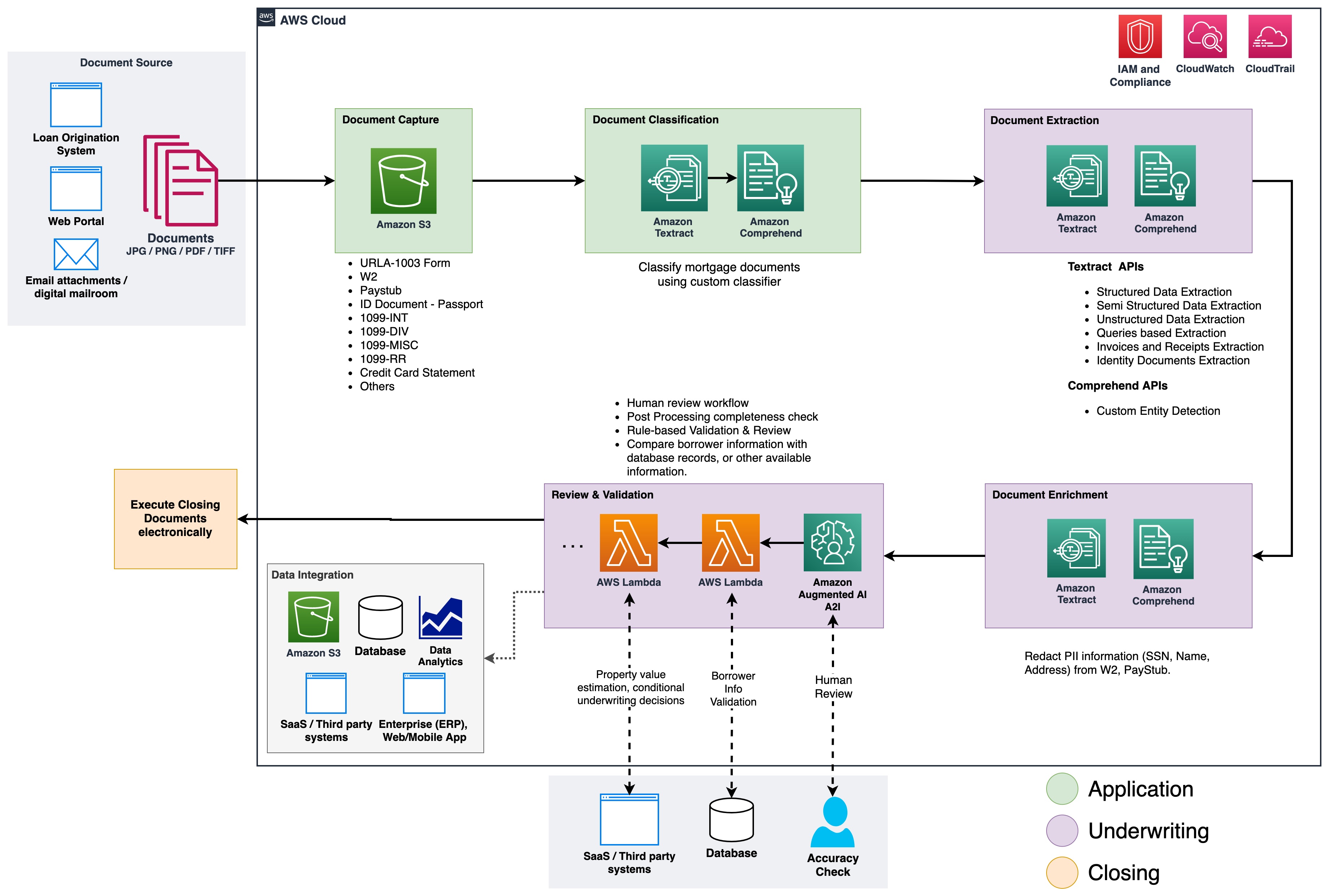
At the start of the process, documents are uploaded to an Amazon Simple Storage Service (Amazon S3) bucket. This initiates a document classification process to categorize the documents into known categories. After the documents are categorized, the next step is to extract key information from them. We then perform enrichment for select documents, which can be things like personally identifiable information (PII) redaction, document tagging, metadata updates, and more. The next step involves validating the data extracted in previous phases to ensure completeness of a mortgage application. Validation can be done via business validation rules and cross document validation rules. The confidence scores of the extracted information can also be compared to a set threshold, and automatically routed to a human reviewer through Amazon Augmented AI (Amazon A2I) if the threshold isn’t met. In the final phase of the process, the extracted and validated data is sent to downstream systems for further storage, processing, or data analytics.

In the following sections, we discuss the phases of IDP as it relates to the phases of a mortgage application in detail. We walk through the phases of IDP and discuss the types of documents; how we store, classify, and extract information, and how we enrich the documents using machine learning.

Document storage

Amazon S3 is an object storage service that offers industry-leading scalability, data availability, security, and performance. We use Amazon S3 to securely store the mortgage documents during and after the mortgage application process. A mortgage application packet may contain several types of forms and documents, such as URLA-1003, 1099-INT/DIV/RR/MISC, W2, paystubs, bank statements, credit card statements, and more. These documents are submitted by the applicant in the mortgage application phase. Without manually looking through them, it might not be immediately clear which documents are included in the packet. This manual process can be time-consuming and expensive. In the next phase, we automate this process using Amazon Comprehend to classify the documents into their respective categories with high accuracy.

Document classification

Document classification is a method by means of which a large number of unidentified documents can be categorized and labeled. We perform this document classification using an Amazon Comprehend custom classifier. A custom classifier is an ML model that can be trained with a set of labeled documents to recognize the classes that are of interest to you. After the model is trained and deployed behind a hosted endpoint, we can utilize the classifier to determine the category (or class) a particular document belongs to. In this case, we train a custom classifier in multi-class mode, which can be done either with a CSV file or an augmented manifest file. For the purposes of this demonstration, we use a CSV file to train the classifier. Refer to our GitHub repository for the full code sample. The following is a high-level overview of the steps involved:

  1. Extract UTF-8 encoded plain text from image or PDF files using the Amazon Textract DetectDocumentText API.
  2. Prepare training data to train a custom classifier in CSV format.
  3. Train a custom classifier using the CSV file.
  4. Deploy the trained model with an endpoint for real-time document classification or use multi-class mode, which supports both real-time and asynchronous operations.

The following diagram illustrates this process.

Image shows Amazon Comprehend custom classifier training process and document classification using the trained and deployed classifier model (real time or batch).

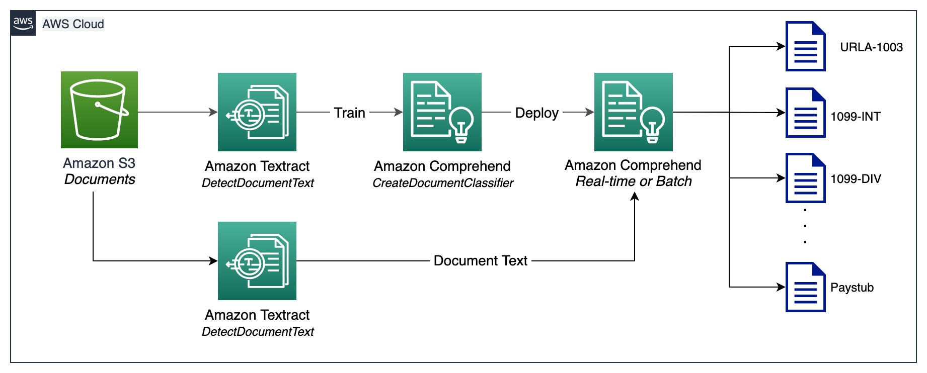
You can automate document classification using the deployed endpoint to identify and categorize documents. This automation is useful to verify whether all the required documents are present in a mortgage packet. A missing document can be quickly identified, without manual intervention, and notified to the applicant much earlier in the process.

Document extraction

In this phase, we extract data from the document using Amazon Textract and Amazon Comprehend. For structured and semi-structured documents containing forms and tables, we use the Amazon Textract AnalyzeDocument API. For specialized documents such as ID documents, Amazon Textract provides the AnalyzeID API. Some documents may also contain dense text, and you may need to extract business-specific key terms from them, also known as entities. We use the custom entity recognition capability of Amazon Comprehend to train a custom entity recognizer, which can identify such entities from the dense text.

In the following sections, we walk through the sample documents that are present in a mortgage application packet, and discuss the methods used to extract information from them. For each of these examples, a code snippet and a short sample output is included.

Extract data from Unified Residential Loan Application URLA-1003

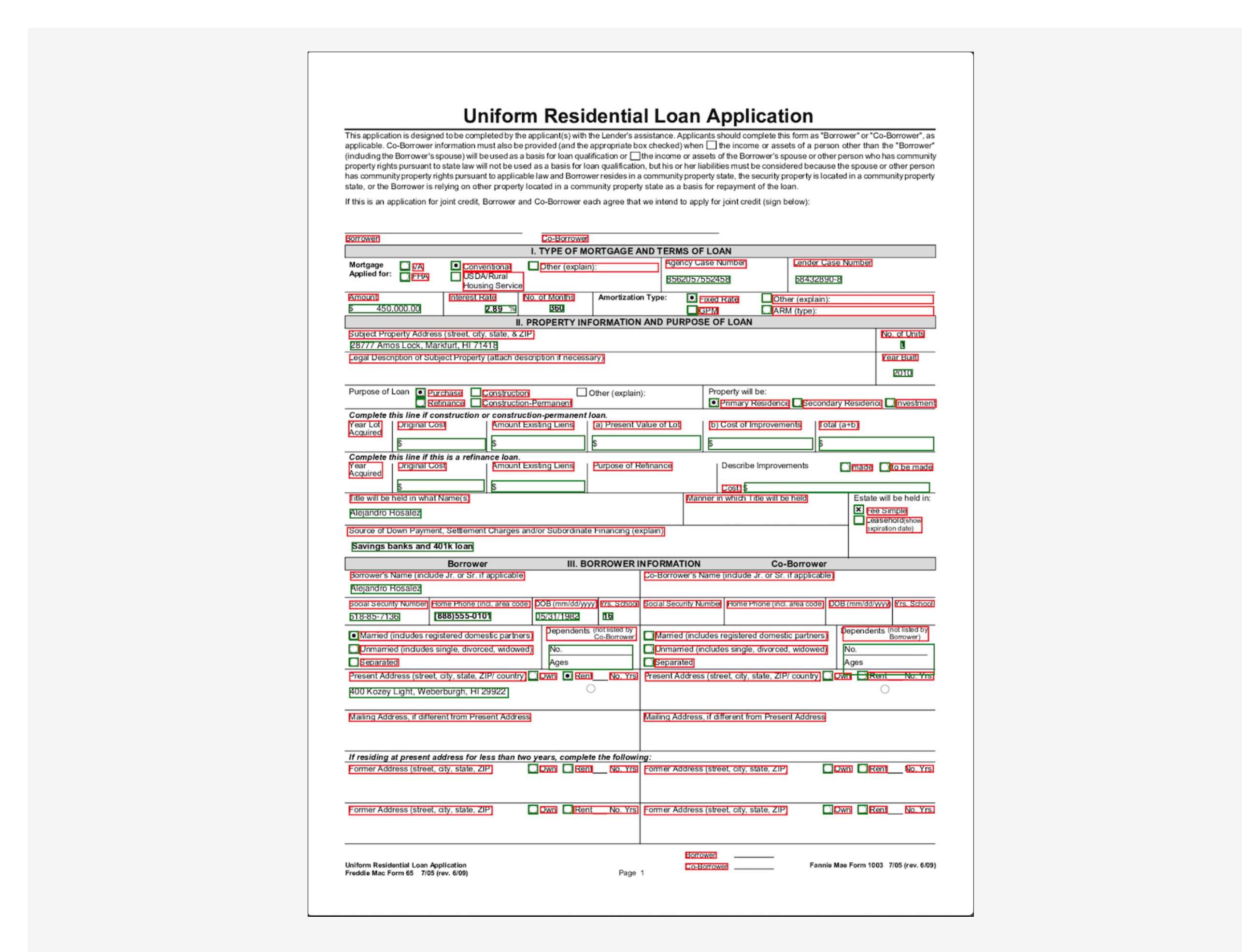
A Unified Residential Loan Application (URLA-1003) is an industry standard mortgage loan application form. It’s a fairly complex document that contains information about the mortgage applicant, type of property being purchased, amount being financed, and other details about the nature of the property purchase. The following is a sample URLA-1003, and our intention is to extract information from this structured document. Because this is a form, we use the AnalyzeDocument API with a feature type of FORM.

Image shows a sample of a Unified Residential Loan Application URLA-1003 form

The FORM feature type extracts form information from the document, which is then returned in key-value pair format. The following code snippet uses the amazon-textract-textractor Python library to extract form information with just a few lines of code. The convenience method call_textract() calls the AnalyzeDocument API internally, and the parameters passed to the method abstract some of the configurations that the API needs to run the extraction task. Document is a convenience method used to help parse the JSON response from the API. It provides a high-level abstraction and makes the API output iterable and easy to get information out of. For more information, refer to Textract Response Parser and Textractor.

from textractcaller.t_call import call_textract, Textract_Features
from trp import Document

response_urla_1003 = call_textract(input_document='s3://<your-bucket>/URLA-1003.pdf', 
                                   features=[Textract_Features.FORMS])
doc_urla_1003 = Document(response_urla_1003)
for page in doc_urla_1003.pages:
    forms=[]
    for field in page.form.fields:
        obj={}
        obj[f'{field.key}']=f'{field.value}'
        forms.append(obj)
print(json.dumps(forms, indent=4))

Note that the output contains values for check boxes or radio buttons that exist in the form. For example, in the sample URLA-1003 document, the Purchase option was selected. The corresponding output for the radio button is extracted as “Purchase” (key) and “SELECTED” (value), indicating that radio button was selected.

[
    { "No. of Units": "1" },
    { "Amount": "$ 450,000.00" },
    { "Year Built": "2010" },
    { "Purchase": "SELECTED" },
    { "Title will be held in what Name(s)": "Alejandro Rosalez" },
    { "Fixed Rate": "SELECTED" },
    ...
]

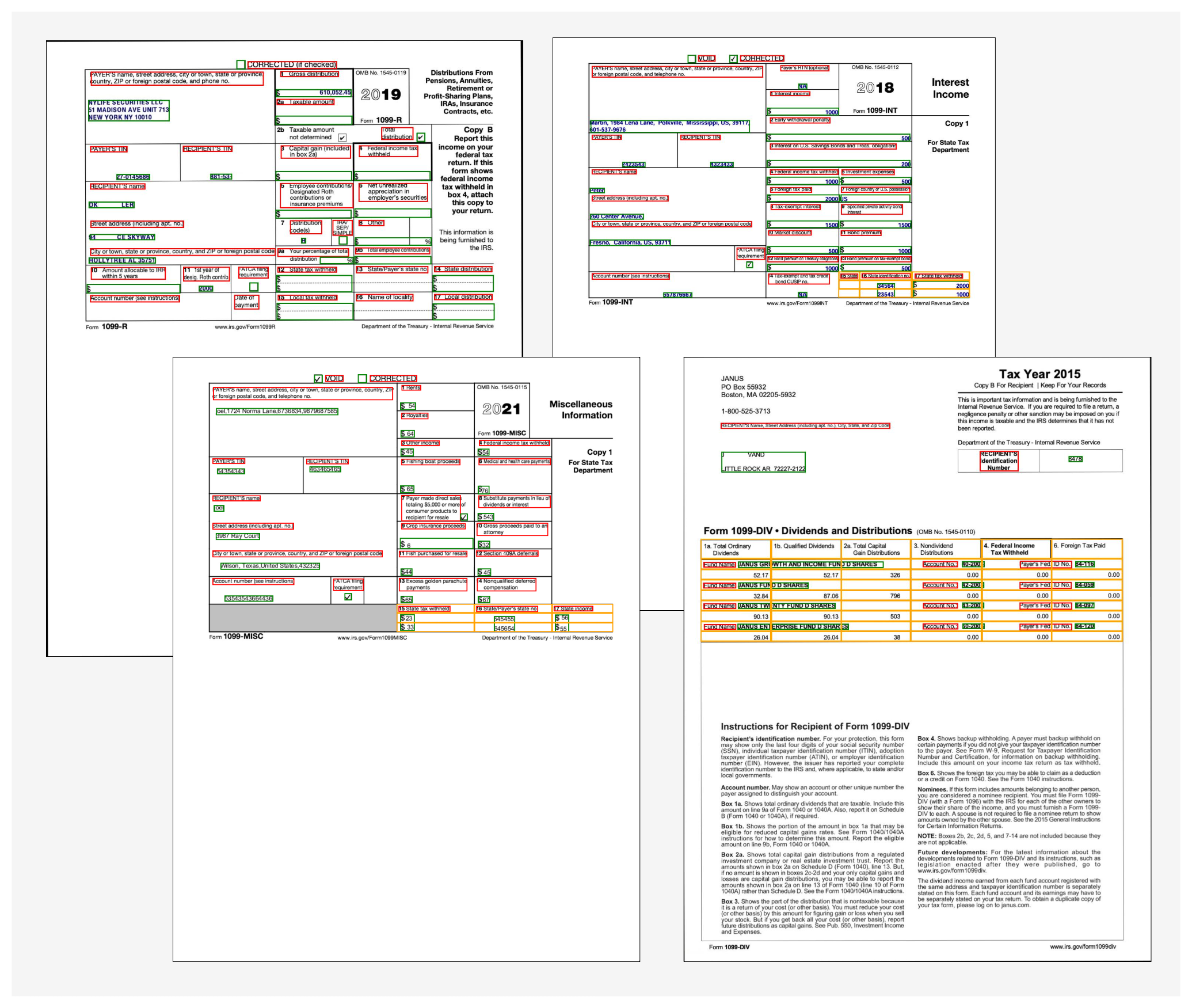
Extract data from 1099 forms

A mortgage application packet may also contain a number of IRS documents, such as 1099-DIV, 1099-INT, 1099-MISC, and 1099-R. These documents show the applicant’s earnings via interests, dividends, and other miscellaneous income components that are useful during underwriting to make decisions. The following image shows a collection of these documents, which are similar in structure. However, in some instances, the documents contain form information (marked using the red and green bounding boxes) as well as tabular information (marked by the yellow bounding boxes).

Image shows samples of 1099 INT, DIV, MISC, and R forms.

To extract form information, we use similar code as explained earlier with the AnalyzeDocument API. We pass an additional feature of TABLE to the API to indicate that we need both form and table data extracted from the document. The following code snippet uses the AnalyzeDocument API with FORMS and TABLES features on the 1099-INT document:

from textractcaller.t_call import call_textract, Textract_Features
from trp import Document
response_1099_int = call_textract(input_document='s3://<your-bucket>/1099-INT-2018.pdf',
                                  features=[Textract_Features.TABLES, 
                                            Textract_Features.FORMS])
doc_1099_int = Document(response_1099_int)
num_tables=1
for page in doc_1099_int.pages:     
    for table in page.tables:
        num_tables=num_tables+1
        for r, row in enumerate(table.rows):
            for c, cell in enumerate(row.cells):
                print(f"Cell[{r}][{c}] = {cell.text}")
        print('n')

Because the document contains a single table, the output of the code is as follows:

Table 1
-------------------
Cell[0][0] = 15 State 
Cell[0][1] = 16 State identification no. 
Cell[0][2] = 17 State tax withheld 
Cell[1][0] = 
Cell[1][1] = 34564 
Cell[1][2] = $ 2000 
Cell[2][0] = 
Cell[2][1] = 23543 
Cell[2][2] = $ 1000

The table information contains the cell position (row 0, column 0, and so on) and the corresponding text within each cell. We use a convenience method that can transform this table data into easy-to-read grid view:

from textractprettyprinter.t_pretty_print import Textract_Pretty_Print, get_string, Pretty_Print_Table_Format
print(get_string(textract_json=response_1099_int, 
                 table_format=Pretty_Print_Table_Format.grid, 
                 output_type=[Textract_Pretty_Print.TABLES]))

We get the following output:

+----------+-----------------------------+-----------------------+
| 15 State | 16 State identification no. | 17 State tax withheld |
+----------+-----------------------------+-----------------------+
|          | 34564                       | $ 2000                |
+----------+-----------------------------+-----------------------+
|          | 23543                       | $ 1000                |
+----------+-----------------------------+-----------------------+

To get the output in an easy-to-consume CSV format, the format type of Pretty_Print_Table_Format.csv can be passed into the table_format parameter. Other formats such as TSV (tab separated values), HTML, and Latex are also supported. For more information, refer to Textract-PrettyPrinter.

Extract data from a mortgage note

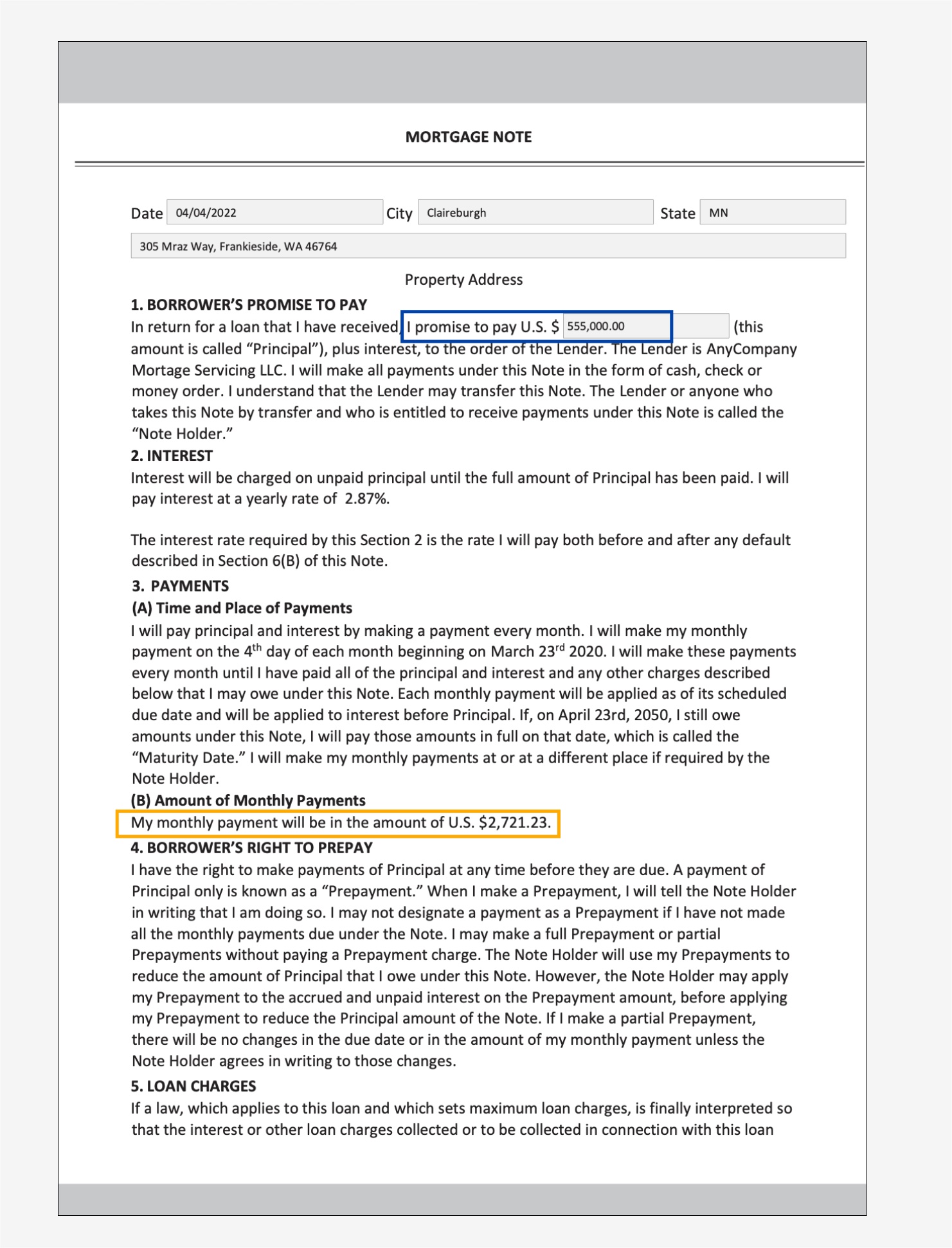
A mortgage application packet may contain unstructured documents with dense text. Some examples of dense text documents are contracts and agreements. A mortgage note is an agreement between a mortgage applicant and the lender or mortgage company, and contains information in dense text paragraphs. In such cases, the lack of structure makes it difficult to find key business information that is important in the mortgage application process. There are two approaches to solving this problem:

In the following sample mortgage note, we’re specifically interested in finding out the monthly payment amount and principal amount.

Image shows a sample of a mortgage note document.

For the first approach, we use the Query and QueriesConfig convenience methods to configure a set of questions that is passed to the Amazon Textract AnalyzeDocument API call. In case the document is multi-page (PDF or TIFF), we can also specify the page numbers where Amazon Textract should look for answers to the question. The following code snippet demonstrates how to create the query configuration, make an API call, and subsequently parse the response to get the answers from the response:

from textractcaller import QueriesConfig, Query
import trp.trp2 as t2

#Setup the queries
query2 = Query(text="What is the principal amount borrower has to pay?", alias="PRINCIPAL_AMOUNT", pages=["1"])
query4 = Query(text="What is the monthly payment amount?", alias="MONTHLY_AMOUNT", pages=["1"])

#Setup the query config with the above queries
queries_config = QueriesConfig(queries=[query1, query2, query3, query4])
#Call AnalyzeDocument with the queries_config
response_mortgage_note = call_textract(input_document='s3://<your-bucket>/Mortgage-Note.pdf',
                                       features=[Textract_Features.QUERIES],
                                       queries_config=queries_config)
doc_mortgage_note: t2.TDocumentSchema = t2.TDocumentSchema().load(response_mortgage_note) 

entities = {}
for page in doc_mortgage_note.pages:
    query_answers = doc_mortgage_note.get_query_answers(page=page)
    if query_answers:
        for answer in query_answers:
            entities[answer[1]] = answer[2]
print(entities)

We get the following output:

{
    'PRINCIPAL_AMOUNT': '$ 555,000.00',
    'MONTHLY_AMOUNT': '$2,721.23',
}

For the second approach, we use the Amazon Comprehend DetectEntities API with the mortgage note, which returns the entities it detects within the text from a predefined set of entities. These are entities that the Amazon Comprehend entity recognizer is pre-trained with. However, because our requirement is to detect specific entities, an Amazon Comprehend custom entity recognizer is trained with a set of sample mortgage note documents, and a list of entities. We define the entity names as PRINCIPAL_AMOUNT and MONTHLY_AMOUNT. Training data is prepared following the Amazon Comprehend training data preparation guidelines for custom entity recognition. The entity recognizer can be trained with document annotations or with entity lists. For the purposes of this example, we use entity lists to train the model. After we train the model, we can deploy it with a real-time endpoint or in batch mode to detect the two entities from the document contents. The following are the steps involved to train a custom entity recognizer and deploy it. For a full code walkthrough, refer to our GitHub repository.

  1. Prepare the training data (the entity list and the documents with (UTF-8 encoded) plain text format).
  2. Start the entity recognizer training using the CreateEntityRecognizer API using the training data.
  3. Deploy the trained model with a real-time endpoint using the CreateEndpoint API.

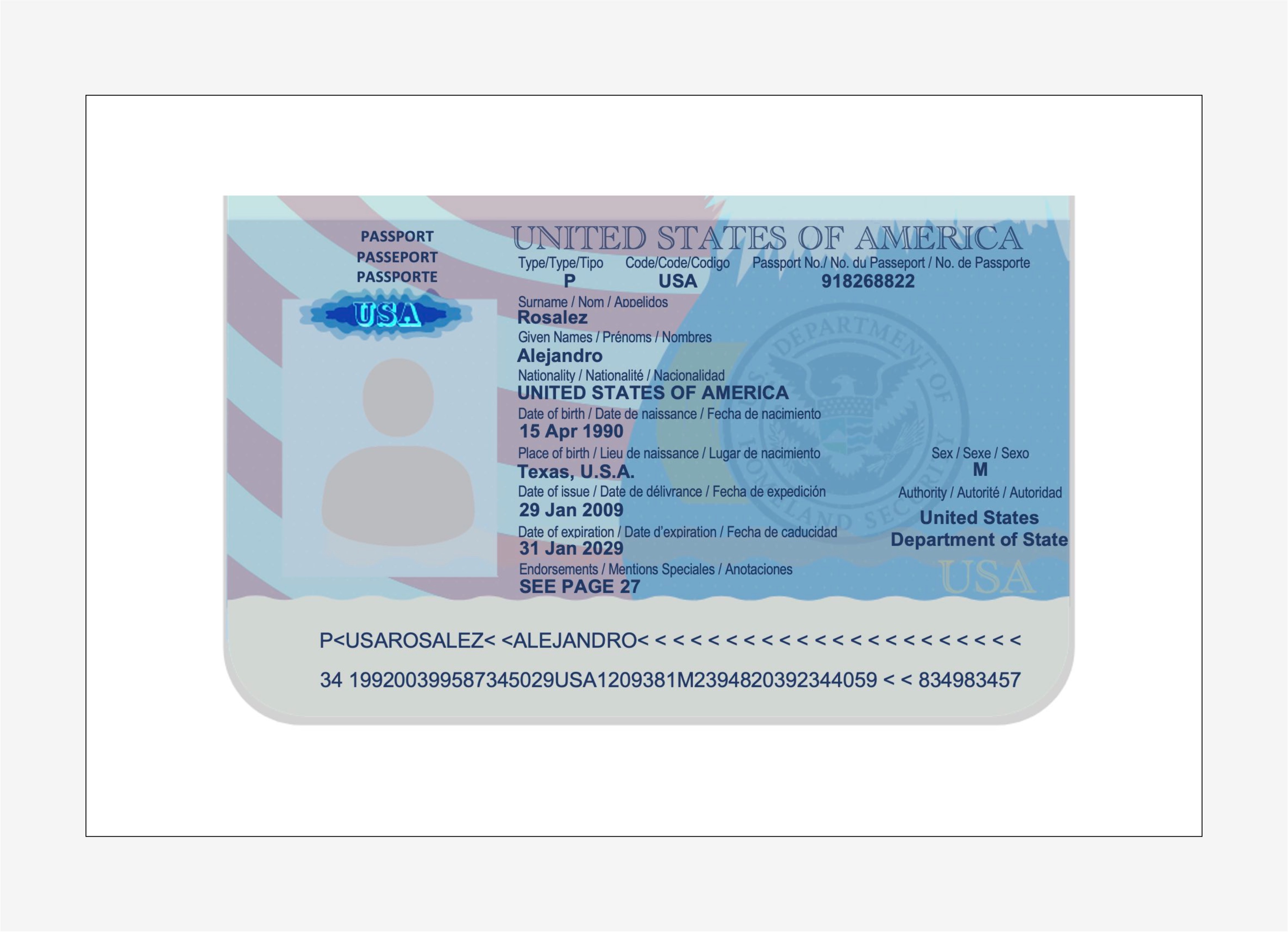
Extract data from a US passport

The Amazon Textract analyze identity documents capability can detect and extract information from US-based ID documents such as a driver’s license and passport. The AnalyzeID API is capable of detecting and interpreting implied fields in ID documents, which makes it easy to extract specific information from the document. Identity documents are almost always part of a mortgage application packet, because it’s used to verify the identity of the borrower during the underwriting process, and to validate the correctness of the borrower’s biographical data.

Image shows a sample of a US passport

We use a convenience method named call_textract_analyzeid, which calls the AnalyzeID API internally. We then iterate over the response to obtain the detected key-value pairs from the ID document. See the following code:

from textractcaller import call_textract_analyzeid
import trp.trp2_analyzeid as t2id

response_passport = call_textract_analyzeid(document_pages=['s3://<your-bucket>/Passport.pdf'])
doc_passport: t2id.TAnalyzeIdDocument = t2id.TAnalyzeIdDocumentSchema().load(response_passport)

for id_docs in response_passport['IdentityDocuments']:
    id_doc_kvs={}
    for field in id_docs['IdentityDocumentFields']:
        if field['ValueDetection']['Text']:
            id_doc_kvs[field['Type']['Text']] = field['ValueDetection']['Text']
print(id_doc_kvs)

AnalyzeID returns information in a structure called IdentityDocumentFields, which contains the normalized keys and their corresponding value. For example, in the following output, FIRST_NAME is a normalized key and the value is ALEJANDRO. In the example passport image, the field for the first name is labeled as “Given Names / Prénoms / Nombre,” however AnalyzeID was able to normalize that into the key name FIRST_NAME. For a list of supported normalized fields, refer to Identity Documentation Response Objects.

{
    'FIRST_NAME': 'ALEJANDRO',
    'LAST_NAME': 'ROSALEZ',
    'DOCUMENT_NUMBER': '918268822',
    'EXPIRATION_DATE': '31 JAN 2029',
    'DATE_OF_BIRTH': '15 APR 1990',
    'DATE_OF_ISSUE': '29 JAN 2009',
    'ID_TYPE': 'PASSPORT',
    'ENDORSEMENTS': 'SEE PAGE 27',
    'PLACE_OF_BIRTH': 'TEXAS U.S.A.'
}

A mortgage packet may contain several other documents, such as a paystub, W2 form, bank statement, credit card statement, and employment verification letter. We have samples for each of these documents along with the code required to extract data from them. For the complete code base, check out the notebooks in our GitHub repository.

Document enrichment

One of the most common forms of document enrichment is sensitive or confidential information redaction on documents, which may be mandated due to privacy laws or regulations. For example, a mortgage applicant’s paystub may contain sensitive PII data, such as name, address, and SSN, that may need redaction for extended storage.

In the preceding sample paystub document, we perform redaction of PII data such as SSN, name, bank account number, and dates. To identify PII data in a document, we use the Amazon Comprehend PII detection capability via the DetectPIIEntities API. This API inspects the content of the document to identify the presence of PII information. Because this API requires input in UTF-8 encoded plain text format, we first extract the text from the document using the Amazon Textract DetectDocumentText API, which returns the text from the document and also returns geometry information such as bounding box dimensions and coordinates. A combination of both outputs is then used to draw redactions on the document as part of the enrichment process.

Review, validate, and integrate data

Extracted data from the document extraction phase may need validation against specific business rules. Specific information may also be validated across several documents, also known as cross-doc validation. An example of cross-doc validation could be comparing the applicant’s name in the ID document to the name in the mortgage application document. You can also do other validations such as property value estimations and conditional underwriting decisions in this phase.

A third type of validation is related to the confidence score of the extracted data in the document extraction phase. Amazon Textract and Amazon Comprehend return a confidence score for forms, tables, text data, and entities detected. You can configure a confidence score threshold to ensure that only correct values are being sent downstream. This is achieved via Amazon A2I, which compares the confidence scores of detected data with a predefined confidence threshold. If the threshold isn’t met, the document and the extracted output is routed to a human for review through an intuitive UI. The reviewer takes corrective action on the data and saves it for further processing. For more information, refer to Core Concepts of Amazon A2I.

Conclusion

In this post, we discussed the phases of intelligent document processing as it relates to phases of a mortgage application. We looked at a few common examples of documents that can be found in a mortgage application packet. We also discussed ways of extracting and processing structured, semi-structured, and unstructured content from these documents. IDP provides a way to automate end-to-end mortgage document processing that can be scaled to millions of documents, enhancing the quality of application decisions, reducing costs, and serving customers faster.

As a next step, you can try out the code samples and notebooks in our GitHub repository. To learn more about how IDP can help your document processing workloads, visit Automate data processing from documents.


About the authors

Anjan Biswas is a Senior AI Services Solutions Architect with focus on AI/ML and Data Analytics. Anjan is part of the world-wide AI services team and works with customers to help them understand, and develop solutions to business problems with AI and ML. Anjan has over 14 years of experience working with global supply chain, manufacturing, and retail organizations and is actively helping customers get started and scale on AWS AI services.

Dwiti Pathak is a Senior Technical Account Manager based out of San Diego. She is focused on helping Semiconductor industry engage in AWS. In her spare time, she likes reading about new technologies and playing board games.

Balaji Puli is a Solutions Architect based in Bay Area, CA. Currently helping select Northwest U.S healthcare life sciences customers accelerate their AWS cloud adoption. Balaji enjoys traveling and loves to explore different cuisines.

Read More

Introducing nvFuser, a deep learning compiler for PyTorch

nvFuser is a Deep Learning Compiler for NVIDIA GPUs that automatically just-in-time compiles fast and flexible kernels to reliably accelerate users’ networks. It provides significant speedups for deep learning networks running on Volta and later CUDA accelerators by generating fast custom “fusion” kernels at runtime. nvFuser is specifically designed to meet the unique requirements of the PyTorch community, and it supports diverse network architectures and programs with dynamic inputs of varying shapes and strides.
In this blog post we’ll describe nvFuser and how it’s used today, show the significant performance improvements it can obtain on models from HuggingFace and TIMM, and look ahead to nvFuser in PyTorch 1.13 and beyond. If you would like to know more about how and why fusion improves the speed of training for Deep Learning networks, please see our previous talks on nvFuser from GTC 2022 and GTC 2021.
nvFuser relies on a graph representation of PyTorch operations to optimize and accelerate. Since PyTorch has an eager execution model, the PyTorch operations users are running are not directly accessible as a whole program that can be optimized by a system like nvFuser. Therefore users must utilize systems built on top of nvFuser which are capable of capturing users programs and translating them into a form that is optimizable by nvFuser. These higher level systems then pass these captured operations to nvFuser, so that nvFuser can optimize the execution of the user’s script for NVIDIA GPUs. There are three systems that capture, translate, and pass user programs to nvFuser for optimization:

  • TorchScript jit.script

    • This system directly parses sections of an annotated python script to translate into its own representation what the user is doing. This system then applies its own version of auto differentiation to the graph, and passes sections of the subsequent forward and backwards graphs to nvFuser for optimization.
  • FuncTorch

    • This system doesn’t directly look at the user python script, instead inserting a mechanism that captures PyTorch operations as they’re being run. We refer to this type of capture system as “trace program acquisition”, since we’re tracing what has been performed. FuncTorch doesn’t perform its own auto differentiation – it simply traces PyTorch’s autograd directly to get backward graphs.
  • TorchDynamo

    • TorchDynamo is another program acquisition mechanism built on top of FuncTorch. TorchDynamo parses the Python bytecode produced from the user script in order to select portions to trace with FuncTorch. The benefit of TorchDynamo is that it’s able to apply decorators to a user’s script, effectively isolating what should be sent to FuncTorch, making it easier for FuncTorch to successfully trace complex Python scripts.

These systems are available for users to interact with directly while nvFuser automatically and seamlessly optimizes performance critical regions of the user’s code. These systems automatically send parsed user programs to nvFuser so nvFuser can:

  1. Analyze the operations being run on GPUs
  2. Plan parallelization and optimization strategies for those operations
  3. Apply those strategies in generated GPU code
  4. Runtime-compile the generated optimized GPU functions
  5. Execute those CUDA kernels on subsequent iterations

It is important to note nvFuser does not yet support all PyTorch operations, and there are still some scenarios that are actively being improved in nvFuser that are discussed herein. However, nvFuser does support many DL performance critical operations today, and the number of supported operations will grow in subsequent PyTorch releases. nvFuser is capable of generating highly specialized and optimized GPU functions for the operations it does have support for. This means nvFuser is able to power new PyTorch systems like TorchDynamo and FuncTorch to combine the flexibility PyTorch is known for with unbeatable performance.

nvFuser Performance

Before getting into how to use nvFuser, in this section we’ll show the improvements in training speed nvFuser provides for a variety of models from the HuggingFace Transformers and PyTorch Image Models (TIMM) repositories and we will discuss current gaps in nvFuser performance that are under development today. All performance numbers in this section were taken using an NVIDIA A100 40GB GPU, and used either FuncTorch alone or Functorch with TorchDynamo.

HuggingFace Transformer Benchmarks

nvFuser can dramatically accelerate training of HuggingFace Transformers when combined with another important optimization (more on that in a moment). Performance improvements can be seen in Figure 1 to range between 1.12x and 1.50x across a subset of popular HuggingFace Transformer networks.

Figure 1: Performance gains of 8 training scenarios from HuggingFace’s Transformer repository. First performance boost in the dark green is due to replacing the optimizer with an NVIDIA Apex fused AdamW optimizer. The light green is due to adding nvFuser. Models were run with batch size and sequence lengths of [64, 128], [8, 512], [2, 1024], [64, 128], [8, 512], [8, src_seql=512, tgt_seql=128], [8, src_seql=1024, tgt_seql=128], and [8, 512] respectively. All networks were run with Automatic Mixed Precision (AMP) enabled with dtype=float16.

While these speedups are significant, it’s important to understand that nvFuser doesn’t (yet) automate everything about running networks quickly. For HuggingFace Transformers, for example, it was important to use the AdamW fused optimizer from NVIDIA’s Apex repository as the optimizer otherwise consumed a large portion of runtime. Using the fused AdamW optimizer to make the network faster exposes the next major performance bottleneck — memory bound operations. These operations are optimized by nvFuser, providing another large performance boost. With the fused optimizer and nvFuser enabled, the training speed of these networks improved between 1.12x to 1.5x.
HuggingFace Transformer models were run with the torch.amp module. (“amp” stands for Automated Mixed Precision, see the “What Every User Should Know about Mixed Precision in PyTorch” blog post for details.) An option to use nvFuser was added to HuggingFace’sTrainer. If you have TorchDynamo installed you can activate it to enable nvFuser in HuggingFace by passing torchdynamo = ‘nvfuser’ to the Trainer class.
nvFuser has great support for normalization kernels and related fusions frequently found in Natural Language Processing (NLP) models, and it is recommended users try nvFuser in their NLP workloads.

PyTorch Image Models (TIMM) Benchmarks

nvFuser, can also significantly reduce the training time of TIMM networks, up to over 1.3x vs. eager PyTorch, and up to 1.44x vs. eager PyTorch when combined with the torch.amp module. Figure 1 shows nvFuser’s speedup without torch.amp, and when torch.amp is used with the NHWC (“channels last”) and NCHW (“channels first”) formats. nvFuser is integrated in TIMM through FuncTorch tracing directly (without TorchDynamo) and can be used by adding the –aot-autograd command line argument when running the TIMM benchmark or training script.

Figure 1: The Y-axis is the performance gain nvFuser provides over not using nvFuser. A value of 1.0 means no change in perf, 2.0 would mean nvFuser is twice as fast, 0.5 would mean nvFuser takes twice the time to run. Square markers are with float16 Automatic Mixed Precision (AMP) and channels first contiguous inputs, circle markers are float32 inputs, and triangles are with float16 AMP and channels last contiguous inputs. Missing data points are due to an error being encountered when tracing.

When running with float32 precision nvFuser provides a 1.12x geometric mean (“geomean”) speedup on TIMM networks, and when running with torch.amp and “channels first” it provides a 1.14x geomean speedup. However, nvFuser currently doesn’t speedup torch.amp and “channels last” training (a .9x geomean regression), so we recommend not using it in those cases. We are actively working on improving “channels last” performance now, and soon we will have two additional optimization strategies (grid persistent optimizations for channels-last normalizations and fast transposes) which we expect will provide speedups comparable to “channels first” in PyTorch version 1.13 and later. Many of nvFuser’s optimizations can also help in inference cases. However, in PyTorch when running inference on small batch sizes, the performance is typically limited by CPU overhead, which nvFuser can’t completely remove or fix. Therefore, typically the most important optimization for inference is to enable CUDA Graphs when possible. Once CUDA Graphs is enabled, then it can also be beneficial to also enable fusion through nvFuser. Performance of inference is shown in Figure 2 and Figure 3. Inference is only run with float16 AMP as it is uncommon to run inference workloads in full float32 precision.

Figure 2: Performance gains of enabling CUDA Graphs, and CUDA Graphs with nvFuser compared to the performance of native PyTorch without CUDA Graphs and nvFuser across TIMM models with float16 AMP, channels first inputs, and a batch size of 1 and 8 respectively. There is a geomean speedup of 2.74x with CUDA Graphs and 2.71x with CUDA Graphs + nvFuser respectively. nvFuser provides a maximum regression of 0.68x and a maximum performance gain of 2.74x (relative to CUDA Graphs without nvFuser). Performance gain is measured relative to the average time per iteration PyTorch takes without CUDA Graphs and without nvFuser. Models are sorted by how much additional performance nvFuser is providing.

Figure 3: Performance gains of enabling CUDA Graphs, and CUDA Graphs with nvFuser compared to the performance of native PyTorch without CUDA Graphs and nvFuser across TIMM models with AMP, channels last inputs, and a batch size of 1 and 8 respectively. There is a geomean speedup of 2.29x with CUDA Graphs and 2.95x with CUDA Graphs + nvFuser respectively. nvFuser provides a maximum regression of 0.86x and a maximum performance gain of 3.82x (relative to CUDA Graphs without nvFuser). Performance gain is measured relative to the average time per iteration PyTorch takes without CUDA Graphs and without nvFuser. Models are sorted by how much additional performance nvFuser is providing.

So far nvFuser performance has not been tuned for inference workloads so its performance benefit is not consistent across all cases. However, there are still many models that benefit significantly from nvFuser during inference and we encourage users to try nvFuser in inference workloads to see if you would benefit today. Performance of nvFuser in inference workloads will improve in the future and if you’re interested in nvFuser in inference workloads please reach out to us on the PyTorch forums.

Getting Started – Accelerate Your Scripts with nvFuser

We’ve created a tutorial demonstrating how to take advantage of nvFuser to accelerate part of a standard transformer block, and how nvFuser can be used to define fast and novel operations. There are still some rough edges in nvFuser that we’re working hard on improving as we’ve outlined in this blog post. However we’ve also demonstrated some great improvements for training speed on multiple networks in HuggingFace and TIMM and we expect there are opportunities in your networks where nvFuser can help today, and many more opportunities it will help in the future.
If you would like to learn more about nvFuser we recommend watching our presentations from NVIDIA’s GTC conference GTC 2022 and GTC 2021.

Read More