Song embeddings are a key component of most music recommendation engines. In this work, we study the hyper-parameter optimization of behavioral song embeddings based on Word2Vec on a selection of downstream tasks, namely next-song recommendation, false neighbor rejection, and artist and genre clustering. We present new optimization objectives and metrics to monitor the effects of hyper-parameter optimization. We show that single-objective optimization can cause side effects on the non optimized metrics and propose a simple multi-objective optimization to mitigate these effects. We find that…Apple Machine Learning Research

What’s new in TensorFlow 2.10?

Posted by the TensorFlow Team
TensorFlow 2.10 has been released! Highlights of this release include user-friendly features in Keras to help you develop transformers, deterministic and stateless initializers, updates to the optimizers API, and new tools to help you load audio data. We’ve also made performance enhancements with oneDNN, expanded GPU support on Windows, and more. This release also marks TensorFlow Decision Forests 1.0! Read on to learn more.
Keras
Expanded, unified mask support for Keras attention layers
Starting from TensorFlow 2.10, mask handling for Keras attention layers, such as tf.keras.layers.Attention, tf.keras.layers.AdditiveAttention, and tf.keras.layers.MultiHeadAttention have been expanded and unified. In particular, we’ve added two features:
Causal attention: All three layers now support a use_causal_mask argument to call (Attention and AdditiveAttention used to take a causal argument to __init__).
Implicit masking: Keras Attention, AdditiveAttention, and MultiHeadAttention layers now support implicit masking (set mask_zero=True in tf.keras.layers.Embedding).
Combined, this simplifies the implementation of any Transformer-style model since getting the masking right is often a tricky part.
A basic Transformer self-attention block can now be written as:
import tensorflow as tf
embedding = tf.keras.layers.Embedding(
input_dim=10,
output_dim=3,
mask_zero=True) # Infer a correct padding mask.
# Instantiate a Keras multi-head attention (MHA) layer,
# a layer normalization layer, and an `Add` layer object.
mha = tf.keras.layers.MultiHeadAttention(key_dim=4, num_heads=1)
layernorm = tf.keras.layers.LayerNormalization()
add = tf.keras.layers.Add()
# Test input.
x = tf.constant([[1, 2, 3, 4, 5, 0, 0, 0, 0],
[1, 2, 1, 0, 0, 0, 0, 0, 0]])
# The embedding layer sets the mask.
x = embedding(x)
# The MHA layer uses and propagates the mask.
a = mha(query=x, key=x, value=x, use_causal_mask=True)
x = add([x, a]) # The `Add` layer propagates the mask.
x = layernorm(x)
# The mask made it through all layers.
print(x._keras_mask)
And here’s the output:
|
> tf.Tensor( > [[ True True True True True False False False False] > [ True True True False False False False False False]], shape=(2, > 9), dtype=bool) |
Try out the new Keras Optimizers API
In the previous release, Tensorflow 2.9, we published a new version of the Keras Optimizer API, in tf.keras.optimizers.experimental, which will replace the current tf.keras.optimizers namespace in TensorFlow 2.11. To prepare for the upcoming formal switch of the optimizer namespace to the new API, we’ve also exported all of the current Keras optimizers under tf.keras.optimizers.legacy in TensorFlow 2.10.
Most users won’t be affected by this change, but please check the API doc to see if any API used in your workflow has changed. If you decide to keep using the old optimizer, please explicitly change your optimizer to corresponding tf.keras.optimizers.legacy.Optimizer.
You can also find more details about new Keras Optimizers in this article.
Deterministic and Stateless Keras initializers
In TensorFlow 2.10, we’ve made Keras initializers (the tf.keras.initializers API) stateless and deterministic, built on top of stateless TF random ops. Starting in TensorFlow 2.10, both seeded and unseeded Keras initializers will always generate the same values every time they are called (for a given variable shape). The stateless initializer enables Keras to support new features such as multi-client model training with DTensor.
|
init = tf.keras.initializers.RandomNormal() a = init((3, 2)) b = init((3, 2)) # a == b init_2 = tf.keras.initializers.RandomNormal(seed=1) c = init_2((3, 2)) d = init_2((3, 2)) # c == d # a != c init_3 = tf.keras.initializers.RandomNormal(seed=1) e = init_3((3, 2)) # e == c init_4 = tf.keras.initializers.RandomNormal() f = init_4((3, 2)) # f != a |
For unseeded initializers (seed=None), a random seed will be created and assigned at initializer creation (different initializer instances get different seeds). An unseeded initializer will raise a warning if it is reused (called) multiple times. This is because it would produce the same values each time, which may not be intended.
BackupAndRestore checkpoints with step level granularity
In the previous release, Tensorflow 2.9, the tf.keras.callbacks.BackupAndRestore Keras callback would backup the model and training state at epoch boundaries. In Tensorflow 2.10, the callback can also backup the model every N training steps. However, keep in mind that when BackupAndRestore is used with tf.distribute.MultiWorkerMirroredStrategy, the distributed dataset iterator state will be reinitialized and won’t be restored when restoring the model. More information and code examples can be found in the migrate the fault tolerance mechanism guide.
Easily generate an audio classification dataset from a directory of audio files
You can now use a new utility, tf.keras.utils.audio_dataset_from_directory, to easily generate audio classification datasets from directories of .wav files. Just sort your audio files into one different directory per file class, and a single line of code will get you a labeled tf.data.Dataset you can pass to a Keras model. You can find an example here.
The EinsumDense layer is no longer experimental
The einsum function is the swiss army knife of linear algebra. It can efficiently and explicitly describe a wide variety of operations. The tf.keras.layers.EinsumDense layer brings some of that power to Keras.
Operations like einsum, einops.rearrange, and the EinsumDense layer operate based on a string “equation” that describes the axes of the inputs and outputs. For EinsumDense the equation lists the axes of the input argument, the axes of the weights, and the axes of the output. A basic Dense layer can be written as:
|
dense = keras.layers.Dense(units=10, activation=’relu’) dense = keras.layers.EinsumDense(‘…i, ij -> …j’, output_shape=(10,), activation=’relu’) |
Notes:
- …i – This only works on the last axis of the input, that axis is called i.
- ij – The weights are a matrix with shape (ij).
- …j – The result sums out the i axis and leaves j.
For example, here is a stack of 5 Dense layers with 10 units each:
|
dense = keras.layers.EinsumDense(‘…i, nij -> …nj’, output_shape=(5,10)) |
Here is a stack of Dense layers, where each one operates on a different input vector:
|
dense = keras.layers.EinsumDense(‘…ni, nij -> …nj’, output_shape=(5,10)) |
Here is a stack of Dense layers where each one operates on each input vector independently:
|
dense = keras.layers.EinsumDense(‘…ni, mij -> …nmj’, output_shape=(None, 5,10)) |
Performance and collaborations
Improved aarch64 CPU performance: ACL/oneDNN integration
We have worked with Arm, AWS, and Linaro to integrate Compute Library for the Arm® Architecture (ACL) with TensorFlow through oneDNN to accelerate performance on aarch64 CPUs. Starting with TensorFlow 2.10, you can try these experimental optimizations by setting the environment variable TF_ENABLE_ONEDNN_OPTS=1 before running your TensorFlow program.
There may be slightly different numerical results due to different computation and floating-point round-off approaches. If this causes issues for you, turn the optimizations off by setting TF_ENABLE_ONEDNN_OPTS=0 before running your program.
To verify that the optimizations are on, look for a message beginning with “oneDNN custom operations are on” in your program log. We welcome feedback on GitHub and the TensorFlow Forum.
Expanded GPU support on Windows
TensorFlow can now leverage a wider range of GPUs on Windows through the TensorFlow-DirectML plug-in. To enable model training on DirectX 12-capable GPUs from vendors such as AMD, Intel, NVIDIA, and Qualcomm, install the plug-in alongside standard TensorFlow CPU packages on native Windows or WSL2. The preview package currently supports a limited number of basic machine learning models, with a goal to increase model coverage in the future. You can view the open-source code and leave feedback at the TensorFlow-DirectML GitHub repository.
New features in tf.data
Create tf.data Dataset from lists of elements
Tensorflow 2.10 introduces a convenient new experimental API tf.data.experimental.from_list which creates a tf.data.Dataset comprising the given list of elements. The returned dataset will produce the items in the list one by one. The functionality is identical to tf.data.Dataset.from_tensor_slices when elements are scalars, but different when elements have structure.
Consider the following example:
|
dataset = tf.data.experimental.from_list([(1, ‘a’), (2, ‘b’), (3, ‘c’)]) list(dataset.as_numpy_iterator()) [(1, ‘a’), (2, ‘b’), (3, ‘c’)] |
In contrast, to get the same output with `from_tensor_slices`, the data needs to be reorganized:
|
dataset = tf.data.Dataset.from_tensor_slices(([1, 2, 3], [‘a’, ‘b’, ‘c’])) list(dataset.as_numpy_iterator()) [(1, ‘a’), (2, ‘b’), (3, ‘c’)] |
Unlike the from_tensor_slices method, from_list supports non-rectangular input (achieving the same with from_tensor_slices requires the use of ragged tensors).
Sharing tf.data service with concurrent trainers
If you run multiple trainers concurrently using the same training data, it could save resources to cache the data in one tf.data service cluster and share the cluster with the trainers. For example, if you use Vizier to tune hyperparameters, the Vizier jobs can run concurrently and share one tf.data service cluster.
To enable this feature, each trainer needs to generate a unique trainer ID, and you pass the trainer ID to tf.data.experimental.service.distribute. Once a job has consumed the data, the data remains in the cache and is re-used by jobs with different trainer_ids. Requests with the same trainer_id do not re-use data. For example:
|
dataset = expensive_computation() dataset = dataset.apply(tf.data.experimental.service.distribute( processing_mode=tf.data.experimental.service.ShardingPolicy.OFF, service=FLAGS.tf_data_service_address, job_name=”job”, cross_trainer_cache=data_service_ops.CrossTrainerCache( trainer_id=trainer_id()))) |
tf.data service uses a sliding-window cache to store shared data. When one trainer consumes data, the data remains in the cache. When other trainers need data, they can get data from the cache instead of repeating the expensive computation. The cache has a bounded size, so some workers may not read the full dataset. To ensure all the trainers get sufficient training data, we require the input dataset to be infinite. This can be achieved, for example, by repeating the dataset and performing random augmentation on the training instances.
TensorFlow Decision Forests 1.0
In conjunction with the release of Tensorflow 2.10, Tensorflow Decision Forests (TF-DF) reaches version 1.0. With this milestone we want to communicate more broadly that Tensorflow Decision Forests has become a more stable and mature library. We’ve improved our documentation and established more comprehensive testing to make sure that TF-DF is ready for professional environments.
The new release of TF-DF also offers a first look at the Javascript and Go APIs for inference of TF-DF models. While these APIs are still in beta, we are actively looking for feedback for them. TF-DF 1.0 improves performance of oblique splits. Oblique splits allow decision trees to express more complex patterns by conditioning on multiple features at the same time – learn more in our Decision Forests class on developers.google.com. Benchmarks and real-world observations show that oblique splits outperform classical axis-aligned splits on the majority of datasets. Finally, the new release includes our latest bug fixes.
Next steps
Check out the release notes for more information. To stay up to date, you can read the TensorFlow blog, follow twitter.com/tensorflow, or subscribe to youtube.com/tensorflow. If you’ve built something you’d like to share, please submit it for our Community Spotlight at goo.gle/TFCS. For feedback, please file an issue on GitHub or post to the TensorFlow Forum. Thank you!
Detect audio events with Amazon Rekognition
When most people think of using machine learning (ML) with audio data, the use case that usually comes to mind is transcription, also known as speech-to-text. However, there are other useful applications, including using ML to detect sounds.
Using software to detect a sound is called audio event detection, and it has a number of applications. For example, suppose you want to monitor the sounds from a noisy factory floor, listening for an alarm bell that indicates a problem with a machine. In a healthcare environment, you can use audio event detection to passively listen for sounds from a patient that indicate an acute health problem. Media workloads are a good fit for this technique, for example to detect when a referee’s whistle is blown in a sports video. And of course, you can use this technique in a variety of surveillance workloads, like listening for a gunshot or the sound of a car crash from a microphone mounted above a city street.
This post describes how to detect sounds in an audio file even if there are significant background sounds happening at the same time. What’s more, perhaps surprisingly, we use computer vision-based techniques to do the detection, using Amazon Rekognition.
Using audio data with machine learning
The first step in detecting audio events is understanding how audio data is represented. For the purposes of this post, we deal only with recorded audio, although these techniques work with streaming audio.
Recorded audio is typically stored as a sequence of sound samples, which measure the intensity of the sound waves that struck the microphone during recording, over time. There are a wide variety of formats with which to store these samples, but a common approach is to store 10,000, 20,000, or even 40,000 samples per second, with each sample being an integer from 0–65535 (two bytes). Because each sample measures only the intensity of sound waves at a particular moment, the sound data generally isn’t helpful for ML processes because it doesn’t have any useful features in its raw state.
To make that data useful, the sound sample is converted into an image called a spectrogram, which is a representation of the audio data that shows the intensity of different frequency bands over time. The following image shows an example.

The X axis of this image represents time, meaning that the left edge of the image is the very start of the sound, and the right edge of the image is the end. Each column of data within the image represents different frequency bands (indicated by the scale on the left side of the image), and the color at each point represents the intensity of that frequency at that moment in time.
Vertical scaling for spectrograms can be changed to other representations. For example, linear scaling means that the Y axis is evenly divided over frequencies, logarithmic scaling uses a log scale, and so forth. The problem with using these representations is that the frequencies in a sound file are usually not evenly distributed, so most of the information we might be interested in ends up being clustered near the bottom of the image (the lower frequencies).
To solve that problem, our sample image is an example of a Mel spectrogram, which is scaled to closely approximate how human beings perceive sound. Notice the frequency indicators along the left side of the image—they give an idea of how they are distributed vertically, and it’s clear that it’s a non-linear scale.
Additionally, we can modify the measurement of intensity by frequency by time to enhance various features of the audio being measured. As with the Y axis scaling that is implemented by a Mel spectrogram, others emphasize features such as the intensity of the 12 distinctive pitch classes that are used to study music (chroma). Another class emphasizes horizonal (harmonic) features or vertical (percussive) features. The type of sound that is being detected should drive the type of spectrogram used for the detection system.
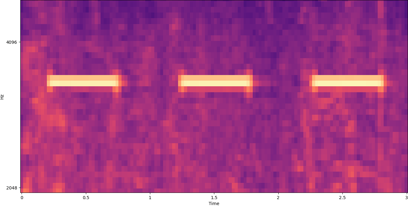
The earlier example spectrogram represents a music clip that is just over 2 minutes long. Zooming in reveals more detail, as is shown in the following image.

The numbers along the top of the image show the number of seconds from the start of the audio file. You can clearly see a sequence of sounds that seems to repeat more than four times per second, indicated by the bright colors near the bottom of the image.
As you can see, this is one of the benefits of converting audio to a spectrogram—distinct sounds are often easily visible with the naked eye, and even if they aren’t, they can frequently be detected using computer vision object detection algorithms. In fact, this is exactly the process we follow in order to detect sounds.
Looking for discrete sounds in a spectrogram
Depending on the length of the audio file that we’re searching, finding a discrete sound that lasts just a second or two is a challenge. Refer to the first spectrogram we shared—because we’re viewing an entire 3:30 minutes of data, details that last only a second or so aren’t visible. We zoomed in a great deal in order to see the rhythm that is shown in the second image. Clearly, with larger sound files (and therefore much larger spectrograms), we quickly run into problems unless we use a different approach. That approach is called windowing.
Windowing refers to using a sliding window that moves across the entire spectrogram, isolating a few seconds (or less) at a time. By repeatedly isolating portions of the overall image, we get smaller images that are searchable for the presence of the sound to be detected. Because each window could result in only part of the image we’re looking for (as in the case of searching for a sound that doesn’t start exactly at the start of a window), windowing is often performed with succeeding windows being overlapped. For example, the first window starts at 0:00 and extends 2 seconds, then the second window starts at 0:01 and extends 2 seconds, and the third window starts at 0:02 and extends 2 seconds, and so on.
Windowing splits a spectrogram image horizontally. We can improve the effectiveness of the detection process by isolating certain frequency bands by cropping or searching only certain vertical parts of the image. For example, if you know that the alarm bell you want to detect creates sounds that range from one specific frequency to another, you can modify the current window to only consider those frequency ranges. That vastly reduces the amount of data to be manipulated, and results in a much faster search. It also improves accuracy, because it’s eliminating possible false positives matches occurring in frequency bands outside of the desired range. The following images compare a full Y axis (left) with a limited Y axis (right).

Full Y Axis |
Limited Y Axis |
Now that we know how to iterate over a spectrogram with a windowing approach and filter to certain frequency bands, the next step is to do the actual search for the sound. For that, we use Amazon Rekognition Custom Labels. The Rekognition Custom Labels feature builds off of the existing capabilities of Amazon Rekognition, which is already trained on tens of millions of images across many categories. Instead of thousands of images, you simply need to upload a small set of training images (typically a few hundred images, but optimal training dataset size should be arrived at experimentally based on the specific use case to avoid under- or over-training the model) that are specific to your use case via the Rekognition Custom Labels console.
If your images are already labeled, Amazon Rekognition training is accessible with just a few clicks. Alternatively, you can label the images directly within the Amazon Rekognition labeling interface, or use Amazon SageMaker Ground Truth to label them for you. When Amazon Rekognition begins training from your image set, it produces a custom image analysis model for you in just a few hours. Behind the scenes, Rekognition Custom Labels automatically loads and inspects the training data, selects the right ML algorithms, trains a model, and provides model performance metrics. You can then use your custom model via the Rekognition Custom Labels API and integrate it into your applications.
Assembling training data and training a Rekognition Custom Labels model
In the GitHub repo associated with this post, you’ll find code that shows how to listen for the sound of a smoke alarm going off, regardless of background noise. In this case, our Rekognition Custom Labels model is a binary classification model, meaning that the results are either “smoke alarm sound was detected” or “smoke alarm sound was not detected.”
To create a custom model, we need training data. That training data is comprised of two main types: environmental sounds, and the sounds you wish to detect (like a smoke alarm going off).
The environmental data should represent a wide variety of soundscapes that are typical for the environment you want to detect the sound in. For example, if you want to detect a smoke alarm sound in a factory environment, start with sounds recorded in that factory environment under a variety of situations (without the smoke alarm sounding, of course).
The sounds you want to detect should be isolated if possible, meaning the recordings should just be the sound itself without any environmental background sounds. For our example, that’s a sound of a smoke alarm going off.
After you’ve collected these sounds, the code in the GitHub repo shows how to combine the environmental sounds with the smoke alarm sounds in various ways (and then convert them to spectrograms) in order to create a number of images that represent the environmental sounds with and without the smoke alarm sounds overlaid on them. The following image is an example of some environmental sounds with a smoke alarm sound (the bright horizontal bars) overlaid on top of it.

The training and test data is stored in an Amazon Simple Storage Service (Amazon S3) bucket. The following directory structure is a good starting point to organize data within the bucket.

The sample code in the GitHub repo allows you to choose how many training images to create. Rekognition Custom Labels doesn’t require a large number of training images. A training set of 200–500 images should be sufficient.
Creating a Rekognition Custom Labels project requires that you specify the URIs of the S3 folder that contains the training data, and (optionally) test data. When specifying the data sources for the training job, one of the options is Automatic labeling, as shown in the following screenshot.

Using this option means that Amazon Rekognition uses the names of the folders as the label names. For our smoke alarm detection use case, the folder structure inside of the train and test folders looks like the following screenshot.
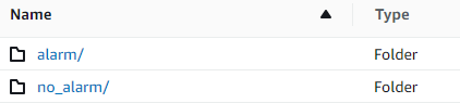
The training data images go into those folders, with spectrograms containing the sound of the smoke alarm going in the alarm folder, and spectrograms that don’t contain the smoke alarm sound in the no_alarm folder. Amazon Rekognition uses those names as the output class names for the custom labels model.
Training a custom label model usually takes 30–90 minutes. At the end of that training, you must start the trained model so it becomes available for use.
End-to-end architecture for sound detection
After we create our model, the next step is to set up an inference pipeline, so we can use the model to detect if a smoke alarm sound is present in an audio file. To do this, the input sound must be turned into a spectrogram and then windowed and filtered by frequency, as was done for the training process. Each window of the spectrogram is given to the model, which returns a classification that indicates if the smoke alarm sounded or not.
The following diagram shows an example architecture that implements this inference pipeline.

This architecture waits for an audio file to be placed into an S3 bucket, which then causes an AWS Lambda function to be invoked. Lambda is a serverless, event-driven compute service that lets you run code for virtually any type of application or backend service without provisioning or managing servers. You can trigger a Lambda function from over 200 AWS services and software as a service (SaaS) applications, and only pay for what you use.
The Lambda function receives the name of the bucket and the name of the key (or file name) of the audio file. The file is downloaded from Amazon S3 to the function’s memory, which then converts it into a spectrogram and performs windowing and frequency filtering. Each windowed portion of the spectrogram is then sent to Amazon Rekognition, which uses the previously-trained Amazon Custom Labels model to detect the sound. If that sound is found, the Lambda function signals that by using an Amazon Simple Notification Service (Amazon SNS) notification. Amazon SNS offers a pub/sub approach where notifications can be sent to Amazon Simple Queue Service (Amazon SQS) queues, Lambda functions, HTTPS endpoints, email addresses, mobile push, and more.
Conclusion
You can use machine learning with audio data to determine when certain sounds occur, even when other sounds are occurring at the same time. Doing so requires converting the sound into a spectrogram image, and then homing in on different parts of that spectrogram by windowing and filtering by frequency band. Rekognition Custom Labels makes it easy to train a custom model for sound detection.
You can use the GitHub repo containing the example code for this post as a starting point for your own experiments. For more information about audio event detection, refer to Sound Event Detection: A Tutorial.
About the authors
 Greg Sommerville is a Senior Prototyping Architect on the AWS Prototyping and Cloud Engineering team, where he helps AWS customers implement innovative solutions to challenging problems with machine learning, IoT and serverless technologies. He lives in Ann Arbor, Michigan and enjoys practicing yoga, catering to his dogs, and playing poker.
 Jeff Harman is a Senior Prototyping Architect on the AWS Prototyping and Cloud Engineering team, where he helps AWS customers implement innovative solutions to challenging problems. He lives in Unionville, Connecticut and enjoys woodworking, blacksmithing, and Minecraft.

Digitizing Smell: Using Molecular Maps to Understand Odor
| Did you ever try to measure a smell? …Until you can measure their likenesses and differences you can have no science of odor. If you are ambitious to found a new science, measure a smell. |
| — Alexander Graham Bell, 1914. |
How can we measure a smell? Smells are produced by molecules that waft through the air, enter our noses, and bind to sensory receptors. Potentially billions of molecules can produce a smell, so figuring out which ones produce which smells is difficult to catalog or predict. Sensory maps can help us solve this problem. Color vision has the most familiar examples of these maps, from the color wheel we each learn in primary school to more sophisticated variants used to perform color correction in video production. While these maps have existed for centuries, useful maps for smell have been missing, because smell is a harder problem to crack: molecules vary in many more ways than photons do; data collection requires physical proximity between the smeller and smell (we don’t have good smell “cameras” and smell “monitors”); and the human eye only has three sensory receptors for color while the human nose has > 300 for odor. As a result, previous efforts to produce odor maps have failed to gain traction.
In 2019, we developed a graph neural network (GNN) model that began to explore thousands of examples of distinct molecules paired with the smell labels that they evoke, e.g., “beefy”, “floral”, or “minty”, to learn the relationship between a molecule’s structure and the probability that such a molecule would have each smell label. The embedding space of this model contains a representation of each molecule as a fixed-length vector describing that molecule in terms of its odor, much as the RGB value of a visual stimulus describes its color.
 |
| Left: An example of a color map (CIE 1931) in which coordinates can be directly translated into values for hue and saturation. Similar colors lie near each other, and specific wavelengths of light (and combinations thereof) can be identified with positions on the map. Right: Odors in the Principal Odor Map operate similarly. Individual molecules correspond to points (grey), and the locations of these points reflect predictions of their odor character. |
Today we introduce the “Principal Odor Map” (POM), which identifies the vector representation of each odorous molecule in the model’s embedding space as a single point in a high-dimensional space. The POM has the properties of a sensory map: first, pairs of perceptually similar odors correspond to two nearby points in the POM (by analogy, red is nearer to orange than to green on the color wheel). Second, the POM enables us to predict and discover new odors and the molecules that produce them. In a series of papers, we demonstrate that the map can be used to prospectively predict the odor properties of molecules, understand these properties in terms of fundamental biology, and tackle pressing global health problems. We discuss each of these promising applications of the POM and how we test them below.
Test 1: Challenging the Model with Molecules Never Smelled Before
First, we asked if the underlying model could correctly predict the odors of new molecules that no one had ever smelled before and that were very different from molecules used during model development. This is an important test — many models perform well on data that looks similar to what the model has seen before, but break down when tested on novel cases.
To test this, we collected the largest ever dataset of odor descriptions for novel molecules. Our partners at the Monell Center trained panelists to rate the smell of each of 400 molecules using 55 distinct labels (e.g., “minty”) that were selected to cover the space of possible smells while being neither redundant nor too sparse. Unsurprisingly, we found that different people had different characterizations of the same molecule. This is why sensory research typically uses panels of dozens or hundreds of people and highlights why smell is a hard problem to solve. Rather than see if the model could match any one person, we asked how close it was to the consensus: the average across all of the panelists. We found that the predictions of the model were closer to the consensus than the average panelist was. In other words, the model demonstrated an exceptional ability to predict odor from a molecule’s structure.
 |
| Predictions made by two models, our GNN model (orange) and a baseline chemoinformatic random forest (RF) model (blue), compared with the mean ratings given by trained panelists (green) for the molecule 2,3-dihydrobenzofuran-5-carboxaldehyde. Each bar corresponds to one odor character label (with only the top 17 of 55 shown for clarity). The top five are indicated in color; our model correctly identifies four of the top five, with high confidence, vs. only three of five, with low confidence, for the RF model. The correlation (R) to the full set of 55 labels is also higher in our model. |
<!–
 |
| Predictions made by two models, our GNN model (orange) and a baseline chemoinformatic random forest (RF) model (blue), compared with the mean ratings given by trained panelists (green) for the molecule 2,3-dihydrobenzofuran-5-carboxaldehyde. Each bar corresponds to one odor character label (with only the top 17 of 55 shown for clarity). The top five are indicated in color; our model correctly identifies four of the top five, with high confidence, vs. only three of five, with low confidence, for the RF model. The correlation (R) to the full set of 55 labels is also higher in our model. |
–>
 |
| Unlike alternative benchmark models (RF and nearest-neighbor models trained on various sets of chemoinformatic features), our GNN model outperforms the median human panelist at predicting the panel mean rating. In other words, our GNN model better reflects the panel consensus than the typical panelist. |
<!–
 |
| Unlike alternative benchmark models (RF and nearest-neighbor models trained on various sets of chemoinformatic features), our GNN model outperforms the median human panelist at predicting the panel mean rating. In other words, our GNN model better reflects the panel consensus than the typical panelist. |
–>
The POM also exhibited state-of-the-art performance on alternative human olfaction tasks like detecting the strength of a smell or the similarity of different smells. Thus, with the POM, it should be possible to predict the odor qualities of any of billions of as-yet-unknown odorous molecules, with broad applications to flavor and fragrance.
Test 2: Linking Odor Quality Back to Fundamental Biology
Because the Principal Odor Map was useful in predicting human odor perception, we asked whether it could also predict odor perception in animals, and the brain activity that underlies it. We found that the map could successfully predict the activity of sensory receptors, neurons, and behavior in most animals that olfactory neuroscientists have studied, including mice and insects.
What common feature of the natural world makes this map applicable to species separated by hundreds of millions of years of evolution? We realized that the common purpose of the ability to smell might be to detect and discriminate between metabolic states, i.e., to sense when something is ripe vs. rotten, nutritious vs. inert, or healthy vs. sick. We gathered data about metabolic reactions in dozens of species across the kingdoms of life and found that the map corresponds closely to metabolism itself. When two molecules are far apart in odor, according to the map, a long series of metabolic reactions is required to convert one to the other; by contrast, similarly smelling molecules are separated by just one or a few reactions. Even long reaction pathways containing many steps trace smooth paths through the map. And molecules that co-occur in the same natural substances (e.g., an orange) are often very tightly clustered on the map. The POM shows that olfaction is linked to our natural world through the structure of metabolism and, perhaps surprisingly, captures fundamental principles of biology.
 |
| Left: We aggregated metabolic reactions found in 17 species across 4 kingdoms to construct a metabolic graph. In this illustration, each circle is a distinct metabolite molecule and an arrow indicates that there is a metabolic reaction that converts one molecule to another. Some metabolites have an odor (color) and others do not (gray), and the metabolic distance between two odorous metabolites is the minimum number of reactions necessary to convert one into the other. In the path shown in bold, the distance is 3. Right: Metabolic distance was highly correlated with distance in the POM, an estimate of perceived odor dissimilarity. |
<!–
 |
| Left: We aggregated metabolic reactions found in 17 species across 4 kingdoms to construct a metabolic graph. In this illustration, each circle is a distinct metabolite molecule and an arrow indicates that there is a metabolic reaction that converts one molecule to another. Some metabolites have an odor (color) and others do not (gray), and the metabolic distance between two odorous metabolites is the minimum number of reactions necessary to convert one into the other. In the path shown in bold, the distance is 3. Right: Metabolic distance was highly correlated with distance in the POM, an estimate of perceived odor dissimilarity. |
–>
Test 3: Extending the Model to Tackle a Global Health Challenge
A map of odor that is tightly connected to perception and biology across the animal kingdom opens new doors. Mosquitos and other insect pests are drawn to humans in part by their odor perception. Since the POM can be used to predict animal olfaction generally, we retrained it to tackle one of humanity’s biggest problems, the scourge of diseases transmitted by mosquitoes and ticks, which kill hundreds of thousands of people each year.
For this purpose, we improved our original model with two new sources of data: (1) a long-forgotten set of experiments conducted by the USDA on human volunteers beginning 80 years ago and recently made discoverable by Google Books, which we subsequently made machine-readable; and (2) a new dataset collected by our partners at TropIQ, using their high-throughput laboratory mosquito assay. Both datasets measure how well a given molecule keeps mosquitos away. Together, the resulting model can predict the mosquito repellency of nearly any molecule, enabling a virtual screen over huge swaths of molecular space. We validated this screen experimentally using entirely new molecules and found over a dozen of them with repellency at least as high as DEET, the active ingredient in most insect repellents. Less expensive, longer lasting, and safer repellents can reduce the worldwide incidence of diseases like malaria, potentially saving countless lives.
 |
| We digitized USDA mosquito repellency data for thousands of molecules previously scanned by Google Books, and used it to refine the learned representation (the map) at the heart of the model. We added additional layers, specifically to predict repellency in a mosquito feeder assay, and iteratively trained the model to improve assay predictions while running computational screens for candidate repellents. |
 |
| Many molecules showing mosquito repellency in the laboratory assay also showed repellency when applied to humans. Several showed repellency greater than the most common repellents used today (DEET and picaridin). |
The Road Ahead
We discovered that our modeling approach to smell prediction could be used to draw a Principal Odor Map for tackling odor-related problems more generally. This map was the key to measuring smell: it answered a range of questions about novel smells and the molecules that produce them, it connected smells back to their origins in evolution and the natural world, and it is helping us tackle important human-health challenges that affect millions of people. Going forward, we hope that this approach can be used to find new solutions to problems in food and fragrance formulation, environmental quality monitoring, and the detection of human and animal diseases.
Acknowledgements
This work was performed by the ML olfaction research team, including Benjamin Sanchez-Lengeling, Brian K. Lee, Jennifer N. Wei, Wesley W. Qian, and Jake Yasonik (the latter two were partly supported by the Google Student Researcher program) and our external partners including Emily Mayhew and Joel D. Mainland from the Monell Center, and Koen Dechering and Marnix Vlot from TropIQ. The Google Books team brought the USDA dataset online. Richard C. Gerkin was supported by the Google Visiting Faculty Researcher program and is also an Associate Research Professor at Arizona State University.
A quick guide to Amazon’s 40-plus papers at Interspeech 2022
Speech recognition and text-to-speech predominate, but other topics include audio watermarking, automatic dubbing, and compression.Read More
Model Teachers: Startups Make Schools Smarter With Machine Learning
Like two valedictorians, SimInsights and Photomath tell stories worth hearing about how AI is advancing education.
SimInsights in Irvine, Calif., uses NVIDIA conversational AI to make virtual and augmented reality classes lifelike for college students and employee training.
Photomath — founded in Zagreb, Croatia and based in San Mateo, Calif. — created an app using computer vision and natural language processing to help students and their parents brush up on everything from arithmetic to calculus.
Both companies are a part of NVIDIA Inception, a free, global program that nurtures cutting-edge startups.
Surfing Sims in California
Rajesh Jha loved simulations since he developed a physics simulation engine for mechanical parts in college, more than 25 years ago. “So, I put sim in the name when I started my own company in 2009,” he said.
SimInsights originally developed web and mobile training simulations. When AR and VR platforms became available, Jha secured a grant to develop HyperSkill. Now the company’s main product, it’s a cloud-based, AI-powered 3D simulation authoring and analytics tool that makes training immersive.
The software helped UCLA’s medical center build a virtual clinic to train students. But they complained about the low accuracy of its rules-based conversational AI, so Jha took data from the first class and trained a deep neural network using NVIDIA Riva, GPU-accelerated software for building speech AI applications.
Riva Revs Up Speech AI
“There was a quick uptick in the quality, and they say it’s the most realistic training they’ve used,” said Jha.
Now, UCLA wants to apply the technology to train thousands of nurses on dealing with infectious diseases.
“There’s a huge role for conversational AI in education and training because it personalizes the experience,” he said. “And a lot of research shows if you can do that, people learn more and retain it longer.”
Access to New Technology
Because SimInsights is an NVIDIA Inception member, it got early access to Riva and NVIDIA TAO, a toolkit that accelerates evaluating and training AI models with transfer learning. They’ve become standard parts of the company’s workflow.
As for Riva, “it’s a powerful piece of software, and our team really appreciates working with NVIDIA to brainstorm our next steps,” Jha said.
Specifically, SimInsights aims to develop larger conversational AI models with more functions, such as question answering so students can point to objects in a scene and ask about them.
“As Riva gives us more capabilities, we’ll incorporate them into HyperSkill to make digital learning as good as working with an expert — it will take a while, but this is the way to get there,” he said.
Accelerating Math in Croatia
In Zagreb, Damir Sabol got stuck trying to help his eldest son understand a math problem in his homework. It sparked the idea for Photomath, an app that’s been downloaded more than 300 million times since its 2015 release.
The app detects an equation in a smartphone picture, then shows step-by-step solutions to it in formats that support different learning styles.
“At peak times, we get thousands of requests a second, so we need to be really fast,” said Ivan Jurin, who leads the startup’s AI projects.
Some teachers have students open the app as an alternative to working on the blackboard. It’s the kind of anecdote that makes Jurin’s day.
“We want to make education more accessible,” he said. “The free version of Photomath can help people who lack resources understand math almost as well as someone who can afford a tutor.”
A Large Hybrid Model
Under the hood, one large neural network does most of the work, detecting and parsing equations. It’s a mix of a convolutional network and a transformer model that packs about 100 million parameters.
It’s trained on local servers with NVIDIA RTX A6000 GPUs. For a cost-sensitive startup, “training in the cloud didn’t motivate us to experiment with larger datasets and more complex models, but with local servers we can queue up experiments as we see fit,” said Vedran Vekić, a senior machine learning engineer at the company.
Once trained, the service runs in the cloud on NVIDIA T4 Tensor Core GPUs, which he described as “very cost effective.”
NVIDIA Software Speeds Inference
The startup is migrating to a full stack of NVIDIA AI software to accelerate inference. It includes NVIDIA Triton Inference Server for maximum throughput, the TensorRT software development kit to minimize latency and NVIDIA DALI, a library for processing images fast.
“We were using the open-source TorchServe, but it wasn’t as efficient as we hoped,” Vekić said. NVIDIA software “gets 100% GPU utilization, so we’re using it on our smaller models and converting our large model to it, too.”
It’s a technical challenge that NVIDIA experts can help address, one of the benefits of being in Inception.
SimInsights and Photomath are among hundreds of startups — out of NVIDIA Inception’s total 10,000+ members — that are making education smarter with machine learning.
To learn more, check out these GTC sessions on NVIDIA Riva, NVIDIA Tao and NVIDIA Triton and TensorRT.
The post Model Teachers: Startups Make Schools Smarter With Machine Learning appeared first on NVIDIA Blog.
Ridiculously Realistic Renders Rule This Week ‘In the NVIDIA Studio’
Editor’s note: This post is part of our weekly In the NVIDIA Studio series, which celebrates featured artists, offers creative tips and tricks, and demonstrates how NVIDIA Studio technology accelerates creative workflows.
Viral creator turned NVIDIA 3D artist Lorenzo Drago takes viewers on a jaw-dropping journey through Toyama, Japan’s Etchū-Daimon Station this week In the NVIDIA Studio.
Drago’s photorealistic recreation of the train station has garnered over 2 million views in under four months, with audiences marveling at the remarkably accurate detail.
“Reality inspires me the most,” said Drago. “Mundane, everyday things always tell a story — they have nuances that are challenging to capture in fantasy.”
Drago started by camera matching in the fSpy open-source software. This process computed the approximate focal length, orientation and position of the camera in 3D space, based on the defined control points chosen from his Etchū-Daimon reference image.
The artist then moved to Blender software to begin the initial blockout, a 3D rough-draft level built with simple 3D shapes without details or polished art assets. The goal of the blockout was to prototype, test and adjust the foundational shapes of the level.
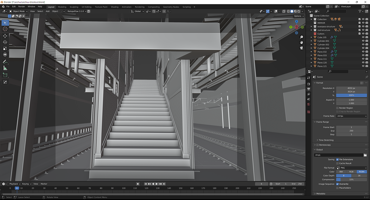
From there, Drago measured the height of a staircase and extrapolated those proportions to the rest of the 3D scene, ensuring it fit the grid size. The scene could then be built modularly, one model at a time. He modeled with lightning speed using NVIDIA RTX-accelerated OptiX ray tracing in the Blender viewport.
Incredibly, the entire scene is a combination of custom-textured assets. Drago’s texturing technique elevated the sense of realism by using tileable textures and trim sheets, which are textures that combine separate details into a single sheet. Mixing these techniques proved to be profitable in creating original, more detailed textures, as well as keeping good pixel density across the scene. Textures never exceeded more than 2048×2048 pixels in size.
Drago created his textures in Adobe Substance 3D Painter, taking advantage of NVIDIA Iray rendering for faster, interactive rendering. RTX acceleration enabled him to quickly bake ambient occlusion and other maps used in texturing, before exporting and applying the textures to the models inside Unreal Engine 5.
Final frame renders came quickly with Drago’s GeForce RTX 2080 SUPER GPU doing the heavy lifting. Drago stressed the necessity of his graphics card.
“For a 3D artist, probably the majority of the work, excluding the planning phases, requires GPU acceleration,” he said. “Being able to work on scenes and objects with materials and lighting rendered in real time saves a lot of time and headaches compared to wireframe or unshaded modes.”
Drago moved on to importing and assembling his textured models in Unreal Engine 5. Elated with the assembly, he began the lighting process. Unreal Engine 5’s Lumen technology enabled lighting iterations in real time, without Drago having to wait for baking or render times.
Unreal Engine’s virtual-reality framework allowed Drago to set up a virtual camera with motion tracking. This gave the animation its signature third-person vantage point, enabling the artist to move around his creative space as if he were holding a smartphone.
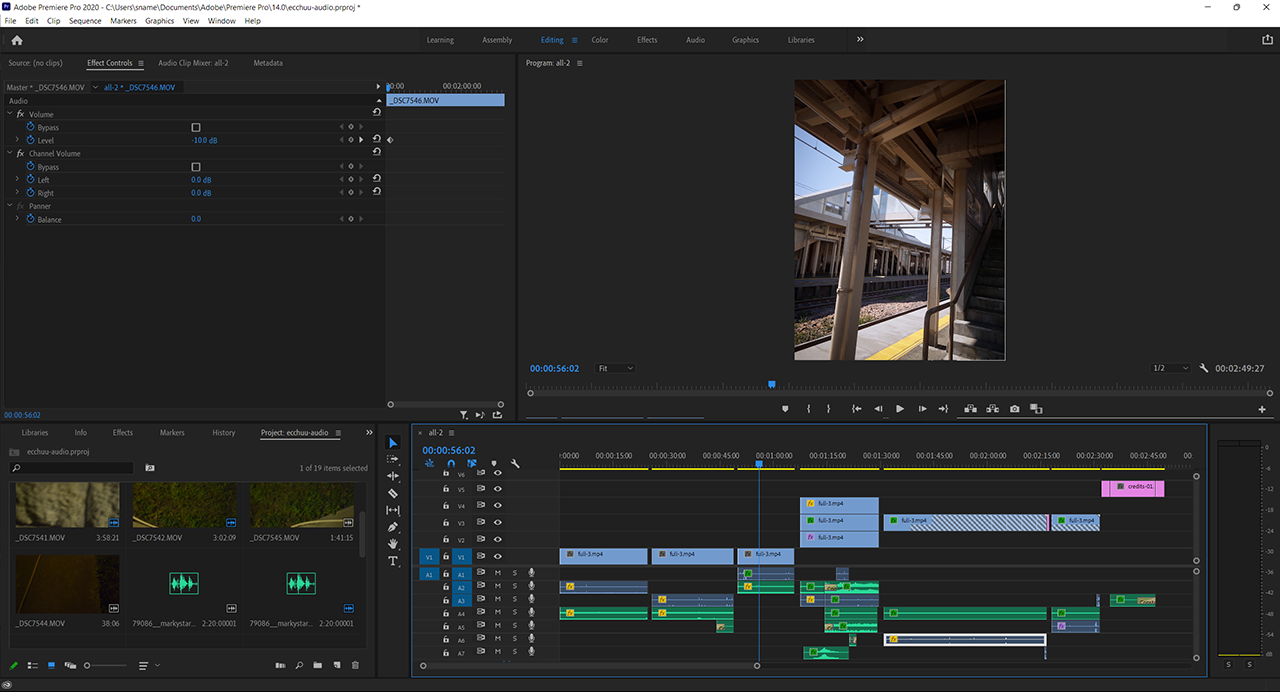
With the renders and animation in place, Drago exported the scene to Adobe Premiere Pro software, where he added sound effects. He also sharpened image details in the animation, one of the many GPU-accelerated features in the software. Drago then deployed GPU-accelerated encoding, NVENC, to speed up the exporting of final files.
Subtle modifications allowed Drago to create ultra-realistic renders. “Mimicking a contemporary smartphone camera — with a limited dynamic range, glare and sharpening artifacts — was a good way of selling the realism,” he said.
“RTX features, like DLSS and ray tracing, are amazing, both from a developer’s point of view and a gamer’s,” Drago stated.

Drago recently imported Etchū-Daimon Station into NVIDIA Omniverse, a 3D design platform for collaborative editing, which replaces linear pipelines with live-sync creation. Drago noted the massive potential within the Omniverse Create App, calling it “a powerful tool capable of achieving extremely high-fidelity results.”
NVIDIA GTC, a global AI conference running online Sept. 19-22, will feature Omniverse sessions with industry experts to demonstrate how the platform can elevate creative workflows. Take advantage of these free resources and register today.
Follow Lorenzo Drago and view his portfolio on ArtStation.
Continue Your Creative Journey
Drago is a self-taught 3D artist, proof that resilience and dedication can lead to incredible, thought provoking, inspirational creative work.
In the spirit of learning, the NVIDIA Studio team is posing a challenge for the community to show off personal growth. Participate in the #CreatorsJourney challenge for a chance to be showcased on NVIDIA Studio social media channels.
Entering is easy. Post an older piece of artwork alongside a more recent one to showcase your growth as an artist. Follow and tag NVIDIA Studio on Instagram, Twitter or Facebook, and use the #CreatorsJourney tag to join.
It’s time to show how you’ve grown as an artist (just like @lowpolycurls)!
Join our #CreatorJourney challenge by sharing something old you created next to something new you’ve made for a chance to be featured on our channels.
Tag #CreatorJourney so we can see your post.
pic.twitter.com/PmkgOvhcBW
— NVIDIA Studio (@NVIDIAStudio) August 15, 2022

There’s more than one way to create incredibly photorealistic visuals. Check out Detailed World Building tutorial by material artist Javier Perez, as well as the three-part series, Create Impressive 360 Panoramic Concept Art, by concept design artist Vladmir Somov. The series showcases a complete workflow in modeling, world building and texturing, and post-processing.
Access free tutorials by industry-leading artists on the Studio YouTube channel. Get creativity-inspiring updates directly to your inbox by subscribing to the NVIDIA Studio newsletter.
The post Ridiculously Realistic Renders Rule This Week ‘In the NVIDIA Studio’ appeared first on NVIDIA Blog.

Analyzing the potential of AlphaFold in drug discovery
Over the past few decades, very few new antibiotics have been developed, largely because current methods for screening potential drugs are prohibitively expensive and time-consuming. One promising new strategy is to use computational models, which offer a potentially faster and cheaper way to identify new drugs.
A new study from MIT reveals the potential and limitations of one such computational approach. Using protein structures generated by an artificial intelligence program called AlphaFold, the researchers explored whether existing models could accurately predict the interactions between bacterial proteins and antibacterial compounds. If so, then researchers could begin to use this type of modeling to do large-scale screens for new compounds that target previously untargeted proteins. This would enable the development of antibiotics with unprecedented mechanisms of action, a task essential to addressing the antibiotic resistance crisis.
However, the researchers, led by James Collins, the Termeer Professor of Medical Engineering and Science in MIT’s Institute for Medical Engineering and Science (IMES) and Department of Biological Engineering, found that these existing models did not perform well for this purpose. In fact, their predictions performed little better than chance.
“Breakthroughs such as AlphaFold are expanding the possibilities for in silico drug discovery efforts, but these developments need to be coupled with additional advances in other aspects of modeling that are part of drug discovery efforts,” Collins says. “Our study speaks to both the current abilities and the current limitations of computational platforms for drug discovery.”
In their new study, the researchers were able to improve the performance of these types of models, known as molecular docking simulations, by applying machine-learning techniques to refine the results. However, more improvement will be necessary to fully take advantage of the protein structures provided by AlphaFold, the researchers say.
Collins is the senior author of the study, which appears today in the journal Molecular Systems Biology. MIT postdocs Felix Wong and Aarti Krishnan are the lead authors of the paper.
Molecular interactions
The new study is part of an effort recently launched by Collins’ lab called the Antibiotics-AI Project, which has the goal of using artificial intelligence to discover and design new antibiotics.
AlphaFold, an AI software developed by DeepMind and Google, has accurately predicted protein structures from their amino acid sequences. This technology has generated excitement among researchers looking for new antibiotics, who hope that they could use the AlphaFold structures to find drugs that bind to specific bacterial proteins.
To test the feasibility of this strategy, Collins and his students decided to study the interactions of 296 essential proteins from E. coli with 218 antibacterial compounds, including antibiotics such as tetracyclines.
The researchers analyzed how these compounds interact with E. coli proteins using molecular docking simulations, which predict how strongly two molecules will bind together based on their shapes and physical properties.
This kind of simulation has been successfully used in studies that screen large numbers of compounds against a single protein target, to identify compounds that bind the best. But in this case, where the researchers were trying to screen many compounds against many potential targets, the predictions turned out to be much less accurate.
By comparing the predictions produced by the model with actual interactions for 12 essential proteins, obtained from lab experiments, the researchers found that the model had false positive rates similar to true positive rates. That suggests that the model was unable to consistently identify true interactions between existing drugs and their targets.
Using a measurement often used to evaluate computational models, known as auROC, the researchers also found poor performance. “Utilizing these standard molecular docking simulations, we obtained an auROC value of roughly 0.5, which basically says you’re doing no better than if you were randomly guessing,” Collins says.
The researchers found similar results when they used this modeling approach with protein structures that have been experimentally determined, instead of the structures predicted by AlphaFold.
“AlphaFold appears to do roughly as well as experimentally determined structures, but we need to do a better job with molecular docking models if we’re going to utilize AlphaFold effectively and extensively in drug discovery,” Collins says.
Better predictions
One possible reason for the model’s poor performance is that the protein structures fed into the model are static, while in biological systems, proteins are flexible and often shift their configurations.
To try to improve the success rate of their modeling approach, the researchers ran the predictions through four additional machine-learning models. These models are trained on data that describe how proteins and other molecules interact with each other, allowing them to incorporate more information into the predictions.
“The machine-learning models learn not just the shapes, but also chemical and physical properties of the known interactions, and then use that information to reassess the docking predictions,” Wong says. “We found that if you were to filter the interactions using those additional models, you can get a higher ratio of true positives to false positives.”
However, additional improvement is still needed before this type of modeling could be used to successfully identify new drugs, the researchers say. One way to do this would be to train the models on more data, including the biophysical and biochemical properties of proteins and their different conformations, and how those features influence their binding with potential drug compounds.
This study both lets us understand just how far we are from realizing full machine-learning-based paradigms for drug development, and provides fantastic experimental and computational benchmarks to stimulate and direct and guide progress towards this future vision,” says Roy Kishony, a professor of biology and computer science at Technion (the Israel Institute of Technology), who was not involved in the study.
With further advances, scientists may be able to harness the power of AI-generated protein structures to discover not only new antibiotics but also drugs to treat a variety of diseases, including cancer, Collins says. “We’re optimistic that with improvements to the modeling approaches and expansion of computing power, these techniques will become increasingly important in drug discovery,” he says. “However, we have a long way to go to achieve the full potential of in silico drug discovery.”
The research was funded by the James S. McDonnell Foundation, the Swiss National Science Foundation, the National Institute of Allergy and Infectious Diseases, the National Institutes of Health, and the Broad Institute of MIT and Harvard. The Antibiotics-AI Project is supported by the Audacious Project, the Flu Lab, the Sea Grape Foundation, and the Wyss Foundation.
Announcing the winners of the 2022 Systems Research request for proposals
For this RFP, we were especially interested in proposals that addressed fundamental challenges that arise in distributed systems operating at a large scale.Read More