Senior principal scientist Jasha Droppo on the shared architectures of large language models and spectrum quantization text-to-speech models — and other convergences between the two fields.Read More
Announcing Amazon S3 access point support for Amazon SageMaker Data Wrangler
We’re excited to announce Amazon SageMaker Data Wrangler support for Amazon S3 Access Points. With its visual point and clikc interface, SageMaker Data Wrangler simplifies the process of data preparation and feature engineering including data selection, cleansing, exploration, and visualization, while S3 Access Points simplifies data access by providing unique hostnames with specific access policies.
Starting today, SageMaker Data Wrangler is making it easier for users to prepare data from shared datasets stored in Amazon Simple Storage Service (Amazon S3) while enabling organizations to securely control data access in their organization. With S3 Access Points, data administrators can now create application- and team-specific access points to facilitate data sharing, rather than managing complex bucket policies with many different permission rules.
In this post, we walk you through importing data from, and exporting data to, an S3 access point in SageMaker Data Wrangler.
Solution Overview
Imagine you, as an administrator, have to manage data for multiple data science teams running their own data preparation workflows in SageMaker Data Wrangler. Administrators often face three challenges:
- Data science teams need to access their datasets without compromising the security of others
- Data science teams need access to some datasets with sensitive data, which further complicates managing permissions
- Security policy only permits data access through specific endpoints to prevent unauthorized access and to reduce the exposure of data
With traditional bucket policies, you would struggle setting up granular access because bucket policies apply the same permissions to all objects within the bucket. Traditional bucket policies also can’t support securing access at the endpoint level.
S3 Access Points solves these problems by granting fine-grained access control at a granular level, making it easier to manage permissions for different teams without impacting other parts of the bucket. Instead of modifying a single bucket policy, you can create multiple access points with individual policies tailored to specific use cases, reducing the risk of misconfiguration or unintended access to sensitive data. Lastly, you can enforce endpoint policies on access points to define rules that control which VPCs or IP addresses can access the data through a specific access point.
We demonstrate how to use S3 Access Points with SageMaker Data Wrangler with the following steps:
- Upload data to an S3 bucket.
- Create an S3 access point.
- Configure your AWS Identity and Access Management (IAM) role with the necessary policies.
- Create a SageMaker Data Wrangler flow.
- Export data from SageMaker Data Wrangler to the access point.
For this post, we use the Bank Marketing dataset for our sample data. However, you can use any other dataset you prefer.
Prerequisites
For this walkthrough, you should have the following prerequisites:
- An AWS account.
- An Amazon SageMaker Studio domain and user. For details on setting these up, refer to Onboard to Amazon SageMaker Domain Using Quick setup.
- An S3 bucket.
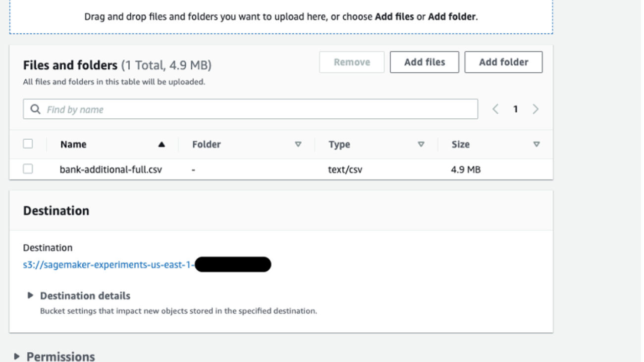
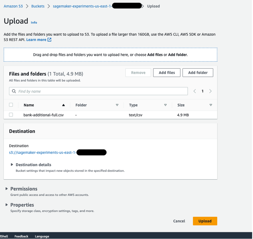
Upload data to an S3 bucket
Upload your data to an S3 bucket. For instructions, refer to Uploading objects. For this post, we use the Bank Marketing dataset.
Create an S3 access point
To create an S3 access point, complete the following steps. For more information, refer to Creating access points.
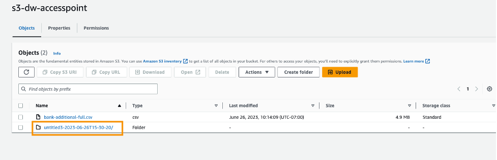
- On the Amazon S3 console, choose Access Points in the navigation pane.
- Choose Create access point.
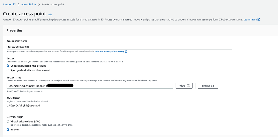
- For Access point name, enter a name for your access point.
- For Bucket, select Choose a bucket in this account.
- For Bucket name, enter the name of the bucket you created.
- Leave the remaining settings as default and choose Create access point.
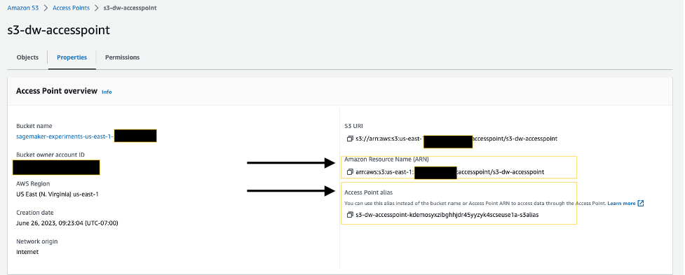
On the access point details page, note the Amazon Resource Name (ARN) and access point alias. You use these later when you interact with the access point in SageMaker Data Wrangler.
Configure your IAM role
If you have a SageMaker Studio domain up and ready, complete the following steps to edit the execution role:
- On the SageMaker console, choose Domains in the navigation pane.
- Choose your domain.
- On the Domain settings tab, choose Edit.
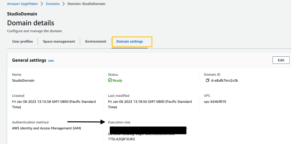
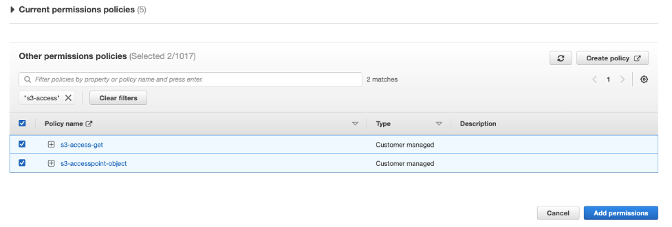
By default, the IAM role that you use to access Data Wrangler is SageMakerExecutionRole. We need to add the following two policies to use S3 access points:
- Policy 1 – This IAM policy grants SageMaker Data Wrangler access to perform
PutObject,GetObject, andDeleteObject:
- Policy 2 – This IAM policy grants SageMaker Data Wrangler access to get the S3 access point:
- Create these two policies and attach them to the role.
Using S3 Access Points in SageMaker Data Wrangler
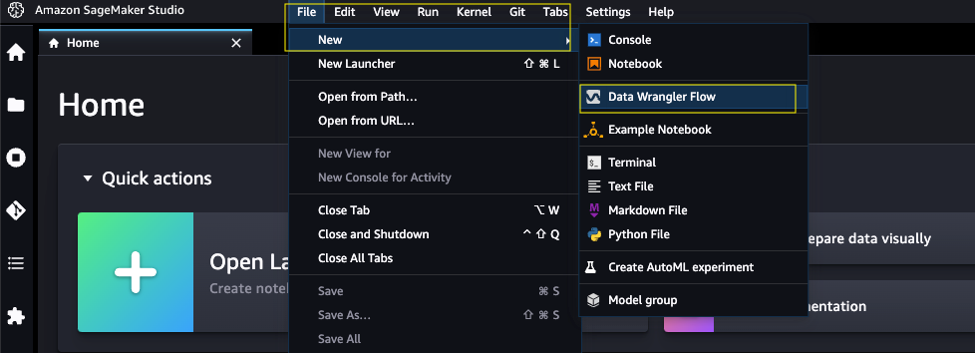
To create a new SageMaker Data Wrangler flow, complete the following steps:
- Launch SageMaker Studio.
- On the File menu, choose New and Data Wrangler Flow.
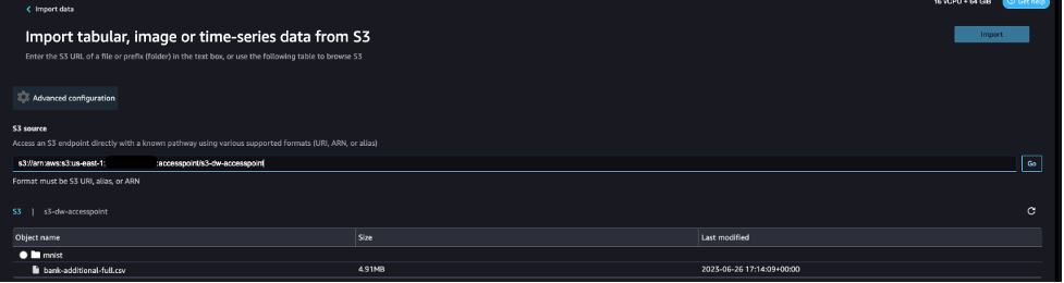
- Choose Amazon S3 as the data source.
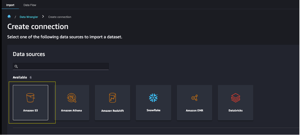
- For S3 source, enter the S3 access point using the ARN or alias that you noted down earlier.
For this post, we use the ARN to import data using the S3 access point. However, the ARN only works for S3 access points and SageMaker Studio domains within the same Region.
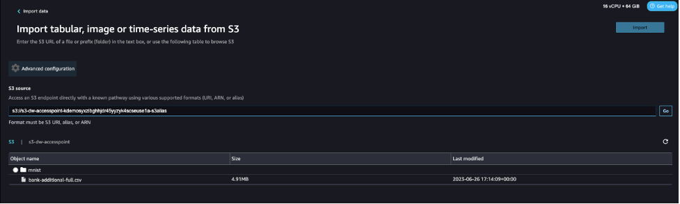
Alternatively, you can use the alias, as shown in the following screenshot. Unlike ARNs, aliases can be referenced across Regions.
Export data from SageMaker Data Wrangler to S3 access points
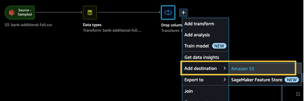
After we complete the necessary transformations, we can export the results to the S3 access point. In our case, we simply dropped a column. When you complete whatever transformations you need for your use case, complete the following steps:
- In the data flow, choose the plus sign.
- Choose Add destination and Amazon S3.
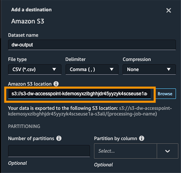
- Enter the dataset name and the S3 location, referencing the ARN.
Now you have used S3 access points to import and export data securely and efficiently without having to manage complex bucket policies and navigate multiple folder structures.
Clean up
If you created a new SageMaker domain to follow along, be sure to stop any running apps and delete your domain to stop incurring charges. Also, delete any S3 access points and delete any S3 buckets.
Conclusion
In this post, we introduced the availability of S3 Access Points for SageMaker Data Wrangler and showed you how you can use this feature to simplify data control within SageMaker Studio. We accessed the dataset from, and saved the resulting transformations to, an S3 access point alias across AWS accounts. We hope that you take advantage of this feature to remove any bottlenecks with data access for your SageMaker Studio users, and encourage you to give it a try!
About the authors
 Peter Chung is a Solutions Architect serving enterprise customers at AWS. He loves to help customers use technology to solve business problems on various topics like cutting costs and leveraging artificial intelligence. He wrote a book on AWS FinOps, and enjoys reading and building solutions.
 Neelam Koshiya is an Enterprise Solution Architect at AWS. Her current focus is to help enterprise customers with their cloud adoption journey for strategic business outcomes. In her spare time, she enjoys reading and being outdoors.

Language to rewards for robotic skill synthesis
Empowering end-users to interactively teach robots to perform novel tasks is a crucial capability for their successful integration into real-world applications. For example, a user may want to teach a robot dog to perform a new trick, or teach a manipulator robot how to organize a lunch box based on user preferences. The recent advancements in large language models (LLMs) pre-trained on extensive internet data have shown a promising path towards achieving this goal. Indeed, researchers have explored diverse ways of leveraging LLMs for robotics, from step-by-step planning and goal-oriented dialogue to robot-code-writing agents.
While these methods impart new modes of compositional generalization, they focus on using language to link together new behaviors from an existing library of control primitives that are either manually engineered or learned a priori. Despite having internal knowledge about robot motions, LLMs struggle to directly output low-level robot commands due to the limited availability of relevant training data. As a result, the expression of these methods are bottlenecked by the breadth of the available primitives, the design of which often requires extensive expert knowledge or massive data collection.
In “Language to Rewards for Robotic Skill Synthesis”, we propose an approach to enable users to teach robots novel actions through natural language input. To do so, we leverage reward functions as an interface that bridges the gap between language and low-level robot actions. We posit that reward functions provide an ideal interface for such tasks given their richness in semantics, modularity, and interpretability. They also provide a direct connection to low-level policies through black-box optimization or reinforcement learning (RL). We developed a language-to-reward system that leverages LLMs to translate natural language user instructions into reward-specifying code and then applies MuJoCo MPC to find optimal low-level robot actions that maximize the generated reward function. We demonstrate our language-to-reward system on a variety of robotic control tasks in simulation using a quadruped robot and a dexterous manipulator robot. We further validate our method on a physical robot manipulator.
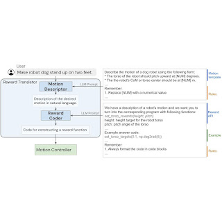
The language-to-reward system consists of two core components: (1) a Reward Translator, and (2) a Motion Controller. The Reward Translator maps natural language instruction from users to reward functions represented as python code. The Motion Controller optimizes the given reward function using receding horizon optimization to find the optimal low-level robot actions, such as the amount of torque that should be applied to each robot motor.
 |
| LLMs cannot directly generate low-level robotic actions due to lack of data in pre-training dataset. We propose to use reward functions to bridge the gap between language and low-level robot actions, and enable novel complex robot motions from natural language instructions. |
Reward Translator: Translating user instructions to reward functions
The Reward Translator module was built with the goal of mapping natural language user instructions to reward functions. Reward tuning is highly domain-specific and requires expert knowledge, so it was not surprising to us when we found that LLMs trained on generic language datasets are unable to directly generate a reward function for a specific hardware. To address this, we apply the in-context learning ability of LLMs. Furthermore, we split the Reward Translator into two sub-modules: Motion Descriptor and Reward Coder.
Motion Descriptor
First, we design a Motion Descriptor that interprets input from a user and expands it into a natural language description of the desired robot motion following a predefined template. This Motion Descriptor turns potentially ambiguous or vague user instructions into more specific and descriptive robot motions, making the reward coding task more stable. Moreover, users interact with the system through the motion description field, so this also provides a more interpretable interface for users compared to directly showing the reward function.
To create the Motion Descriptor, we use an LLM to translate the user input into a detailed description of the desired robot motion. We design prompts that guide the LLMs to output the motion description with the right amount of details and format. By translating a vague user instruction into a more detailed description, we are able to more reliably generate the reward function with our system. This idea can also be potentially applied more generally beyond robotics tasks, and is relevant to Inner-Monologue and chain-of-thought prompting.
Reward Coder
In the second stage, we use the same LLM from Motion Descriptor for Reward Coder, which translates generated motion description into the reward function. Reward functions are represented using python code to benefit from the LLMs’ knowledge of reward, coding, and code structure.
Ideally, we would like to use an LLM to directly generate a reward function R (s, t) that maps the robot state s and time t into a scalar reward value. However, generating the correct reward function from scratch is still a challenging problem for LLMs and correcting the errors requires the user to understand the generated code to provide the right feedback. As such, we pre-define a set of reward terms that are commonly used for the robot of interest and allow LLMs to composite different reward terms to formulate the final reward function. To achieve this, we design a prompt that specifies the reward terms and guide the LLM to generate the correct reward function for the task.
 |
| The internal structure of the Reward Translator, which is tasked to map user inputs to reward functions. |
Motion Controller: Translating reward functions to robot actions
The Motion Controller takes the reward function generated by the Reward Translator and synthesizes a controller that maps robot observation to low-level robot actions. To do this, we formulate the controller synthesis problem as a Markov decision process (MDP), which can be solved using different strategies, including RL, offline trajectory optimization, or model predictive control (MPC). Specifically, we use an open-source implementation based on the MuJoCo MPC (MJPC).
MJPC has demonstrated the interactive creation of diverse behaviors, such as legged locomotion, grasping, and finger-gaiting, while supporting multiple planning algorithms, such as iterative linear–quadratic–Gaussian (iLQG) and predictive sampling. More importantly, the frequent re-planning in MJPC empowers its robustness to uncertainties in the system and enables an interactive motion synthesis and correction system when combined with LLMs.
Examples
Robot dog
In the first example, we apply the language-to-reward system to a simulated quadruped robot and teach it to perform various skills. For each skill, the user will provide a concise instruction to the system, which will then synthesize the robot motion by using reward functions as an intermediate interface.
Dexterous manipulator
We then apply the language-to-reward system to a dexterous manipulator robot to perform a variety of manipulation tasks. The dexterous manipulator has 27 degrees of freedom, which is very challenging to control. Many of these tasks require manipulation skills beyond grasping, making it difficult for pre-designed primitives to work. We also include an example where the user can interactively instruct the robot to place an apple inside a drawer.
Validation on real robots
We also validate the language-to-reward method using a real-world manipulation robot to perform tasks such as picking up objects and opening a drawer. To perform the optimization in Motion Controller, we use AprilTag, a fiducial marker system, and F-VLM, an open-vocabulary object detection tool, to identify the position of the table and objects being manipulated.
Conclusion
In this work, we describe a new paradigm for interfacing an LLM with a robot through reward functions, powered by a low-level model predictive control tool, MuJoCo MPC. Using reward functions as the interface enables LLMs to work in a semantic-rich space that plays to the strengths of LLMs, while ensuring the expressiveness of the resulting controller. To further improve the performance of the system, we propose to use a structured motion description template to better extract internal knowledge about robot motions from LLMs. We demonstrate our proposed system on two simulated robot platforms and one real robot for both locomotion and manipulation tasks.
Acknowledgements
We would like to thank our co-authors Nimrod Gileadi, Chuyuan Fu, Sean Kirmani, Kuang-Huei Lee, Montse Gonzalez Arenas, Hao-Tien Lewis Chiang, Tom Erez, Leonard Hasenclever, Brian Ichter, Ted Xiao, Peng Xu, Andy Zeng, Tingnan Zhang, Nicolas Heess, Dorsa Sadigh, Jie Tan, and Yuval Tassa for their help and support in various aspects of the project. We would also like to acknowledge Ken Caluwaerts, Kristian Hartikainen, Steven Bohez, Carolina Parada, Marc Toussaint, and the greater teams at Google DeepMind for their feedback and contributions.
Automatically generating labeled training images
Inverting generative adversarial networks to learn label assignments enables a high-quality labeled-image generator that’s trained on 50 images or fewer.Read More
Machine learning with decentralized training data using federated learning on Amazon SageMaker
Machine learning (ML) is revolutionizing solutions across industries and driving new forms of insights and intelligence from data. Many ML algorithms train over large datasets, generalizing patterns it finds in the data and inferring results from those patterns as new unseen records are processed. Usually, if the dataset or model is too large to be trained on a single instance, distributed training allows for multiple instances within a cluster to be used and distribute either data or model partitions across those instances during the training process. Native support for distributed training is offered through the Amazon SageMaker SDK, along with example notebooks in popular frameworks.
However, sometimes due to security and privacy regulations within or across organizations, the data is decentralized across multiple accounts or in different Regions and it can’t be centralized into one account or across Regions. In this case, federated learning (FL) should be considered to get a generalized model on the whole data.
In this post, we discuss how to implement federated learning on Amazon SageMaker to run ML with decentralized training data.
What is federated learning?
Federated learning is an ML approach that allows for multiple separate training sessions running in parallel to run across large boundaries, for example geographically, and aggregate the results to build a generalized model (global model) in the process. More specifically, each training session uses its own dataset and gets its own local model. Local models in different training sessions will be aggregated (for example, model weight aggregation) into a global model during the training process. This approach stands in contrast to centralized ML techniques where datasets are merged for one training session.
Federated learning vs. distributed training on the cloud
When these two approaches are running on the cloud, distributed training happens in one Region on one account, and training data starts with a centralized training session or job. During distributed training process, the dataset gets split into smaller subsets and, depending on the strategy (data parallelism or model parallelism), subsets are sent to different training nodes or go through nodes in a training cluster, which means individual data doesn’t necessarily stay in one node of the cluster.
In contrast, with federated learning, training usually occurs in multiple separate accounts or across Regions. Each account or Region has its own training instances. The training data is decentralized across accounts or Regions from the beginning to the end, and individual data is only read by its respective training session or job between different accounts or Regions during the federated learning process.
Flower federated learning framework
Several open-source frameworks are available for federated learning, such as FATE, Flower, PySyft, OpenFL, FedML, NVFlare, and Tensorflow Federated. When choosing an FL framework, we usually consider its support for model category, ML framework, and device or operation system. We also need to consider the FL framework’s extensibility and package size so as to run it on the cloud efficiently. In this post, we choose an easily extensible, customizable, and lightweight framework, Flower, to do the FL implementation using SageMaker.
Flower is a comprehensive FL framework that distinguishes itself from existing frameworks by offering new facilities to run large-scale FL experiments, and enables richly heterogeneous FL device scenarios. FL solves challenges related to data privacy and scalability in scenarios where sharing data is not possible.
Design principles and implementation of Flower FL
Flower FL is language-agnostic and ML framework-agnostic by design, is fully extensible, and can incorporate emerging algorithms, training strategies, and communication protocols. Flower is open-sourced under Apache 2.0 License.
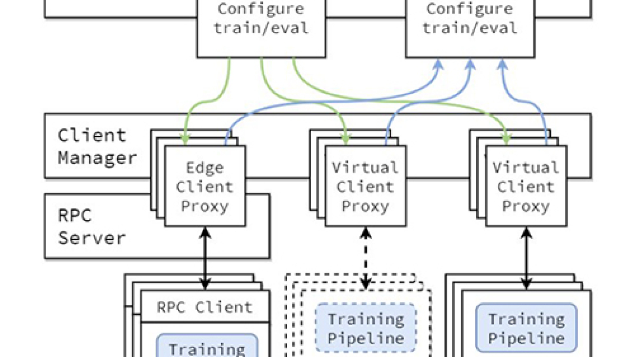
The conceptual architecture of the FL implementation is described in the paper Flower: A friendly Federated Learning Framework and is highlighted in the following figure.
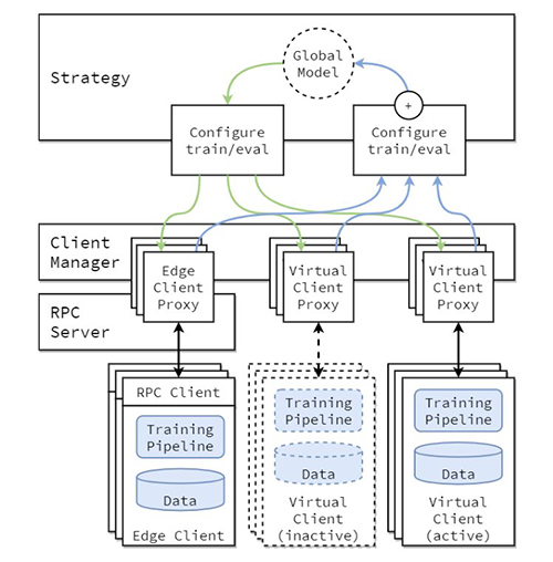
In this architecture, edge clients live on real edge devices and communicate with the server over RPC. Virtual clients, on the other hand, consume close to zero resources when inactive and only load model and data into memory when the client is being selected for training or evaluation.
The Flower server builds the strategy and configurations to be sent to the Flower clients. It serializes these configuration dictionaries (or config dict for short) to their ProtoBuf representation, transports them to the client using gRPC, and then deserializes them back to Python dictionaries.
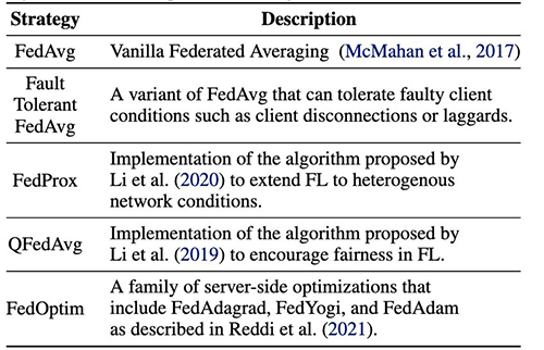
Flower FL strategies
Flower allows customization of the learning process through the strategy abstraction. The strategy defines the entire federation process specifying parameter initialization (whether it’s server or client initialized), the minimum number of clients available required to initialize a run, the weight of the client’s contributions, and training and evaluation details.
Flower has an extensive implementation of FL averaging algorithms and a robust communication stack. For a list of averaging algorithms implemented and associated research papers, refer to the following table, from Flower: A friendly Federated Learning Framework.
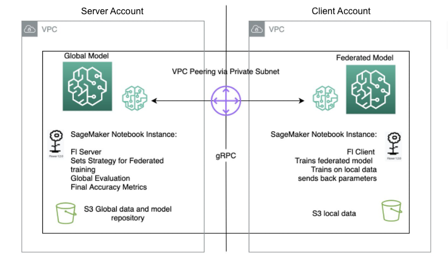
Federated learning with SageMaker: Solution architecture
A federated learning architecture using SageMaker with the Flower framework is implemented on top of bi-directional gRPC (foundation) streams. gRPC defines the types of messages exchanged and uses compilers to then generate efficient implementation for Python, but it can also generate the implementation for other languages, such as Java or C++.
The Flower clients receive instructions (messages) as raw byte arrays via the network. Then the clients deserialize and run the instruction (training on local data). The results (model parameters and weights) are then serialized and communicated back to the server.
The server/client architecture for Flower FL is defined in SageMaker using notebook instances in different accounts in the same Region as the Flower server and Flower client. The training and evaluation strategies are defined on the server as well as the global parameters, then the configuration is serialized and sent to the client over VPC peering.
The notebook instance client starts a SageMaker training job that runs a custom script to trigger the instantiation of the Flower client, which deserializes and reads the server configuration, triggers the training job, and sends the parameters response.
The last step occurs on the server when the evaluation of the newly aggregated parameters is triggered upon completion of the number of runs and clients stipulated on the server strategy. The evaluation takes place on a testing dataset existing only on the server, and the new improved accuracy metrics are produced.
The following diagram illustrates the architecture of the FL setup on SageMaker with the Flower package.
Implement federated learning using SageMaker
SageMaker is a fully managed ML service. With SageMaker, data scientists and developers can quickly build and train ML models, and then deploy them into a production-ready hosted environment.
In this post, we demonstrate how to use the managed ML platform to provide a notebook experience environment and perform federated learning across AWS accounts, using SageMaker training jobs. The raw training data never leaves the account that owns the data and only the derived weights are sent across the peered connection.
We highlight the following core components in this post:
- Networking – SageMaker allows for quick setup of default networking configuration while also allowing you to fully customize the networking depending on your organization’s requirements. We use a VPC peering configuration within the Region in this example.
- Cross-account access settings – In order to allow a user in the server account to start a model training job in the client account, we delegate access across accounts using AWS Identity and Access Management (IAM) roles. This way, a user in the server account doesn’t have to sign out of the account and sign in to the client account to perform actions on SageMaker. This setting is only for purposes of starting SageMaker training jobs, and it doesn’t have any cross-account data access permission or sharing.
- Implementing federated learning client code in the client account and server code in the server account – We implement federated learning client code in the client account by using the Flower package and SageMaker managed training. Meanwhile, we implement server code in the server account by using the Flower package.
Set up VPC peering
A VPC peering connection is a networking connection between two VPCs that enables you to route traffic between them using private IPv4 addresses or IPv6 addresses. Instances in either VPC can communicate with each other as if they are within the same network.
To set up a VPC peering connection, first create a request to peer with another VPC. You can request a VPC peering connection with another VPC in the same account, or in our use case, connect with a VPC in a different AWS account. To activate the request, the owner of the VPC must accept the request. For more details about VPC peering, refer to Create a VPC peering connection.
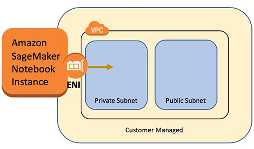
Launch SageMaker notebook instances in VPCs
A SageMaker notebook instance provides a Jupyter notebook app through a fully managed ML Amazon Elastic Compute Cloud (Amazon EC2) instance. SageMaker Jupyter notebooks are used to perform advanced data exploration, create training jobs, deploy models to SageMaker hosting, and test or validate your models.
The notebook instance has a variety of networking configurations available to it. In this setup, we have the notebook instance run within a private subnet of the VPC and don’t have direct internet access.
Configure cross-account access settings
Cross-account access settings include two steps to delegate access from the server account to client account by using IAM roles:
- Create an IAM role in the client account.
- Grant access to the role in the server account.
For detailed steps to set up a similar scenario, refer to Delegate access across AWS accounts using IAM roles.
In the client account, we create an IAM role called FL-kickoff-client-job with the policy FL-sagemaker-actions attached to the role. The FL-sagemaker-actions policy has JSON content as follows:
We then modify the trust policy in the trust relationships of the FL-kickoff-client-job role:
In the server account, permissions are added to an existing user (for example, developer) to allow switching to the FL-kickoff-client-job role in client account. To do this, we create an inline policy called FL-allow-kickoff-client-job and attach it to the user. The following is the policy JSON content:
Sample dataset and data preparation
In this post, we use a curated dataset for fraud detection in Medicare providers’ data released by the Centers for Medicare & Medicaid Services (CMS). Data is split into a training dataset and a testing dataset. Because the majority of the data is non-fraud, we apply SMOTE to balance the training dataset, and further split the training dataset into training and validation parts. Both the training and validation data are uploaded to an Amazon Simple Storage Service (Amazon S3) bucket for model training in the client account, and the testing dataset is used in the server account for testing purposes only. Details of the data preparation code are in the following notebook.
With the SageMaker pre-built Docker images for the scikit-learn framework and SageMaker managed training process, we train a logistic regression model on this dataset using federated learning.
Implement a federated learning client in the client account
In the client account’s SageMaker notebook instance, we prepare a client.py script and a utils.py script. The client.py file contains code for the client, and the utils.py file contains code for some of the utility functions that will be needed for our training. We use the scikit-learn package to build the logistic regression model.
In client.py, we define a Flower client. The client is derived from the class fl.client.NumPyClient. It needs to define the following three methods:
- get_parameters – It returns the current local model parameters. The utility function
get_model_parameterswill do this. - fit – It defines the steps to train the model on the training data in client’s account. It also receives global model parameters and other configuration information from the server. We update the local model’s parameters using the received global parameters and continue training it on the dataset in the client account. This method also sends the local model’s parameters after training, the size of the training set, and a dictionary communicating arbitrary values back to the server.
- evaluate – It evaluates the provided parameters using the validation data in the client account. It returns the loss together with other details such as the size of the validation set and accuracy back to the server.
The following is a code snippet for the Flower client definition:
We then use SageMaker script mode to prepare the rest of the client.py file. This includes defining parameters that will be passed to SageMaker training, loading training and validation data, initializing and training the model on the client, setting up the Flower client to communicate with the server, and finally saving the trained model.
utils.py includes a few utility functions that are called in client.py:
- get_model_parameters – It returns the scikit-learn LogisticRegression model parameters.
- set_model_params – It sets the model’s parameters.
- set_initial_params – It initializes the parameters of the model as zeros. This is required because the server asks for initial model parameters from the client at launch. However, in the scikit-learn framework,
LogisticRegressionmodel parameters are not initialized untilmodel.fit()is called. - load_data – It loads the training and testing data.
- save_model – It saves model as a
.joblibfile.
Because Flower is not a package installed in the SageMaker pre-built scikit-learn Docker container, we list flwr==1.3.0 in a requirements.txt file.
We put all three files (client.py, utils.py, and requirements.txt) under a folder and tar zip it. The .tar.gz file (named source.tar.gz in this post) is then uploaded to an S3 bucket in the client account.
Implement a federated learning server in the server account
In the server account, we prepare code on a Jupyter notebook. This includes two parts: the server first assumes a role to start a training job in the client account, then the server federates the model using Flower.
Assume a role to run the training job in the client account
We use the Boto3 Python SDK to set up an AWS Security Token Service (AWS STS) client to assume the FL-kickoff-client-job role and set up a SageMaker client so as to run a training job in the client account by using the SageMaker managed training process:
Using the assumed role, we create a SageMaker training job in client account. The training job uses the SageMaker built-in scikit-learn framework. Note that all S3 buckets and the SageMaker IAM role in the following code snippet are related to the client account:
Aggregate local models into a global model using Flower
We prepare code to federate the model on the server. This includes defining the strategy for federation and its initialization parameters. We use utility functions in the utils.py script described earlier to initialize and set model parameters. Flower allows you to define your own callback functions to customize an existing strategy. We use the FedAvg strategy with custom callbacks for evaluation and fit configuration. See the following code:
The following two functions are mentioned in the preceding code snippet:
- fit_round – It’s used to send the round number to the client. We pass this callback as the
on_fit_config_fnparameter of the strategy. We do this simply to demonstrate the use of theon_fit_config_fnparameter. - get_evaluate_fn – It’s used for model evaluation on the server.
For demo purposes, we use the testing dataset that we set aside in data preparation to evaluate the model federated from the client’s account and communicate the result back to the client. However, it’s worth noting that in almost all real use cases, the data used in the server account is not split from the dataset used in the client account.
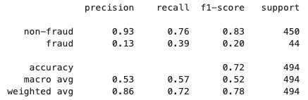
After the federated learning process is finished, a model.tar.gz file is saved by SageMaker as a model artifact in an S3 bucket in the client account. Meanwhile, a model.joblib file is saved on the SageMaker notebook instance in the server account. Lastly, we use the testing dataset to test the final model (model.joblib) on the server. Testing output of the final model is as follows:
Clean up
After you are done, clean up the resources in both the server account and client account to avoid additional charges:
- Stop the SageMaker notebook instances.
- Delete VPC peering connections and corresponding VPCs.
- Empty and delete the S3 bucket you created for data storage.
Conclusion
In this post, we walked through how to implement federated learning on SageMaker by using the Flower package. We showed how to configure VPC peering, set up cross-account access, and implement the FL client and server. This post is useful for those who need to train ML models on SageMaker using decentralized data across accounts with restricted data sharing. Because the FL in this post is implemented using SageMaker, it’s worth noting that a lot more features in SageMaker can be brought into the process.
Implementing federated learning on SageMaker can take advantage of all the advanced features that SageMaker provides through the ML lifecycle. There are other ways to achieve or apply federated learning on the AWS Cloud, such as using EC2 instances or on the edge. For details about these alternative approaches, refer to Federated Learning on AWS with FedML and Applying Federated Learning for ML at the Edge.
About the authors
 Sherry Ding is a senior AI/ML specialist solutions architect at Amazon Web Services (AWS). She has extensive experience in machine learning with a PhD degree in computer science. She mainly works with public sector customers on various AI/ML-related business challenges, helping them accelerate their machine learning journey on the AWS Cloud. When not helping customers, she enjoys outdoor activities.
 Lorea Arrizabalaga is a Solutions Architect aligned to the UK Public Sector, where she helps customers design ML solutions with Amazon SageMaker. She is also part of the Technical Field Community dedicated to hardware acceleration and helps with testing and benchmarking AWS Inferentia and AWS Trainium workloads.
 Ben Snively is an AWS Public Sector Senior Principal Specialist Solutions Architect. He works with government, non-profit, and education customers on big data, analytical, and AI/ML projects, helping them build solutions using AWS.

Coming This Fall: NVIDIA DLSS 3.5 for Chaos Vantage, D5 Render, Omniverse and Popular Game Titles
Editor’s note: This post is part of our weekly In the NVIDIA Studio series, which celebrates featured artists, offers creative tips and tricks, and demonstrates how NVIDIA Studio technology improves creative workflows. We’re also deep diving on new GeForce RTX 40 Series GPU features, technologies and resources, and how they dramatically accelerate content creation.
Gamescom, the biggest gaming event of the year, kicks off tomorrow in Cologne, Germany, but gamers and content creators can find some of the latest innovations, tools and AI-powered tech this week In the NVIDIA Studio.
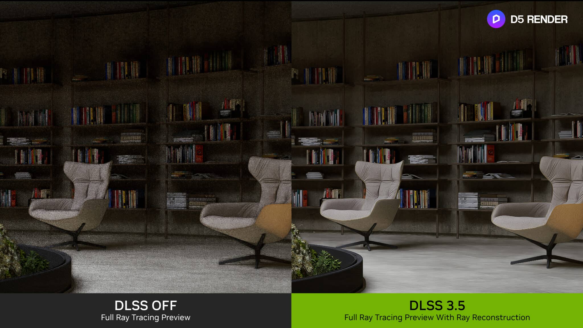
On the eve of the show’s official opening, NVIDIA announced NVIDIA DLSS 3.5 featuring Ray Reconstruction — a new neural rendering AI model that creates more beautiful and realistic ray-traced visuals than traditional rendering methods — for real-time 3D creative apps and games.
NVIDIA RTX Remix, a free modding platform built on NVIDIA Omniverse and available now, gives people the tools to create and share #RTXON mods for classic games. We also announced Half-Life 2 RTX: An RTX Remix Project, a community remaster project of Valve’s Half-Life 2, one of the highest-rated games of all time.
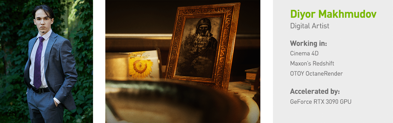
This week’s In the NVIDIA Studio installment also features digital artist Diyor Makhmudov’s 3D work, inspired by the extraordinary gaming franchise The Witcher.
Reallusion software released an update to the iClone Omniverse Connector, including real-time synchronization of projects and enhanced import functionality for OpenUSD, enabling quicker, more efficient workflows. Learn more in the latest edition of the Into the Omniverse series.
Finally, calling all video editors to sign up for the premiere DaVinci Resolve event — ResolveCon — in Portland, Oregon, from Aug. 25-27. In-person attendees can win giveaways, including new GeForce RTX GPUs, while virtual attendees can view tutorials livestreamed by In the NVIDIA Studio artist Casey Faris.
Next-Level Graphical Fidelity With DLSS 3.5
NVIDIA DLSS 3.5 adds Ray Reconstruction, which improves ray-traced image quality for all GeForce RTX GPUs by replacing hand-tuned denoisers with an NVIDIA supercomputer-trained AI network that generates higher-quality pixels in between sampled rays.
Seeing is believing — watch the Tech Talk with NVIDIA Vice President of Applied Deep Learning Research Bryan Catanzaro to learn how DLSS 3.5 works.
Creative apps with ray-traced renderers face a wide variety of content that is difficult for traditional denoisers to handle, as they require hand-tuning for every scene. As a result, content previews return suboptimal image quality. With DLSS 3.5, the AI neural network recognizes a wide variety of scenes, producing high-quality images during preview and before committing hours to a final render.
D5 Render and Chaos Vantage, two popular professional-grade 3D apps for architects and designers, feature real-time preview modes with ray tracing. With DLSS 3.5, the AI neural network replaces the denoisers, inferring and producing higher-quality previews while building and iterating.
Popular creative apps Chaos Vantage, D5 Render and NVIDIA Omniverse, as well as popular gaming titles Alan Wake 2, Cyberpunk 2077, Cyberpunk 2077: Phantom Liberty and Portal with RTX, are all adding support for NVIDIA DLSS 3.5 this fall.
Developers will be able to seamlessly integrate DLSS 3.5 with the new Streamline SDK coming soon. Learn more about DLSS 3.5.
Half-Life 2 RTX: An RTX Remix Project
Half-Life 2 RTX: An RTX Remix Project is being developed by four of Half-Life 2’s top mod teams, now known as Orbifold Studios.

Using the latest version of RTX Remix, Orbifold Studios is rebuilding materials with physically based rendering properties, adding extra geometric detail with Valve’s Hammer editor and using the full range of NVIDIA technologies, including NVIDIA DLSS, NVIDIA RTX IO and NVIDIA Reflex, to breathe new life into the critically acclaimed title.
As with Portal with RTX, a high-fidelity reimagining of Valve’s timeless classic, and Portal: Prelude RTX, built by community modders, nearly every asset in Half-Life 2 RTX: An RTX Remix Project is being reconstructed in high fidelity and with full ray tracing (otherwise known as path tracing, enabling advanced rendering techniques. Compared to the original, some assets feature 20x the geometric detail.
Half-Life 2 RTX: An RTX Remix Project is early in development and is a community effort looking to galvanize talented modders and artists everywhere. To join the project, apply via the Orbifold Studios website.
Eat. Sleep. Game. Create. Repeat.
Already building 3D scenes in immaculate detail, 19-year-old digital creator and 3D lighting artist Diyorbek Makhmudov has the savvy skills of an industry veteran and a bright future ahead.

Makhmudov has always had a deep-rooted passion for gaming, gaining inspiration from the 3D worlds of his favorite games. Most notably, The Witcher franchise has fueled him to create 3D worlds that showcase his own signature look and feel.

Unlike many content creators featured In the NVIDIA Studio, Makhmudov doesn’t like to bring his own life experience into the creative process, enjoying the escapism offered by world-building.
“I like to immerse myself in another universe,” said Makhmudov. “I don’t like to express my feelings, thoughts or emotions in my creations.”

Makhmudov follows standard 3D creative workflow practices: gathering reference material, prepping materials, shaping environments and tinkering with materials, textures and colors. But it’s in 3D creation where he really shines.
Makhmudov uses his preferred 3D app — Cinema 4D — to achieve smooth interactivity while working with complex 3D models thanks to the NVIDIA GPU-accelerated viewport. It’s powered by a GeForce RTX 3090 graphics card, which offers considerable increases in efficiency while fueling creativity.
In the video above, Makhmudov is able to move within the scene, tinkering while the scene renders in real time.
Cinema 4D also supports several popular GPU-accelerated renderers such as Chaos V-Ray, OTOY OctaneRender and Maxon’s Redshift. This flexibility allows Makhmudov to use whichever best suits his needs.

“Redshift is fast, has a good light-linking system and I have almost full control over everything,” said Makhmudov. He prefers OctaneRender for exporting ultra-realistic renders quickly. The built-in Cinema 4D render is also a speedy option. The only thing he can’t do is work on a CPU alone because, to quote Makhmudov, “It’s very slow.”

“When you do personal work, it pushes you more to achieve a good result,” said Makhmudov. “As a bonus, that big portfolio will be a major advantage in your job search.”
Check out Makhmudov on ArtStation.
Follow NVIDIA Studio on Instagram, Twitter and Facebook. Access tutorials on the Studio YouTube channel and get updates directly in your inbox by subscribing to the Studio newsletter.
Get started with NVIDIA Omniverse by downloading the standard license free, or learn how Omniverse Enterprise can connect your team. Developers can get started with Omniverse resources. Stay up to date on the platform by subscribing to the newsletter, and follow NVIDIA Omniverse on Instagram, Medium and Twitter.
For more, join the Omniverse community and check out the Omniverse forums, Discord server, Twitch and YouTube channels.

NVIDIA Debuts AI-Enhanced Real-Time Ray Tracing for Games and Apps With New DLSS 3.5
The latest advancements in AI for gaming are in the spotlight today at Gamescom, the world’s largest gaming conference, as NVIDIA introduced a host of technologies, starting with DLSS 3.5, the next step forward of its breakthrough AI neural rendering technology.
DLSS 3.5, NVIDIA’s latest innovation in AI-powered graphics is an image quality upgrade incorporated into the fall’s hottest ray-traced titles, from Cyberpunk 2077: Phantom Liberty to Alan Wake 2 to Portal with RTX.
But NVIDIA didn’t stop there. DLSS is coming to more AAA blockbusters; emotion is being added to AI-powered non-playable characters (NPCs); Xbox Game Pass titles are coming to the GeForce NOW cloud-gaming service; and upgrades to GeForce NOW servers are underway.
DLSS 3.5 Introduces Ray Reconstruction
The biggest news? The introduction of Ray Reconstruction in DLSS 3.5, a groundbreaking feature that elevates ray-traced image quality for all GeForce RTX GPUs, outclassing traditional hand-tuned denoisers with an AI network trained by an NVIDIA supercomputer.
The result improves lighting effects like reflections, global illumination, and shadows to create a more immersive, realistic gaming experience.
Denoising is used in ray-traced computer graphics to fill in missing pixels to more efficiently composite a final image. NVIDIA DLSS 3.5 is trained on 5x more training data than DLSS 3, so it can recognize different ray-traced effects and make smarter decisions about when to use temporal and spatial data.
DLSS, first released in February 2019, has gotten a number of major upgrades improving both image quality and performance.
Ray Reconstruction is now included as part of DLSS 3.5, which offers a suite of AI rendering technologies powered by Tensor Cores on GeForce RTX GPUs for faster frame rates, better image quality, and great responsiveness.
DLSS 3.5 includes Ray Reconstruction, Super Resolution, Deep Learning Anti-Aliasing and Frame Generation.
NVIDIA announced that upcoming blockbusters Alan Wake 2, Cyberpunk 2077: Phantom Liberty and Portal with RTX will use NVIDIA DLSS 3.5 this fall.
DLSS 3.5 also improves image quality in real-time 3D creator applications and allows 3D creator professionals to showcase a higher-quality image without spending minutes or hours for the final render.
Ray Reconstruction will be included in upcoming releases of D5 Render, Chaos Vantage and NVIDIA Omniverse, a development platform for connecting and building 3D tools and applications.
DLSS is now featured in over 330 games and apps. And this fall’s biggest blockbusters will launch with DLSS 3, including Call of Duty: Modern Warfare III, PAYDAY 3 and Fortnite.
NVIDIA Reflex Comes to More Games
In addition, Call of Duty: Modern Warfare III, PAYDAY 3, Alan Wake 2, Cyberpunk 2077: Phantom Liberty and more will launch with NVIDIA Reflex, which reduces system latency so gamers’ actions occur quicker, providing a competitive edge in multiplayer matches and making single-player titles more responsive and enjoyable.
And Reflex is already increasing gamers’ competitiveness in the latest editions of wildly popular franchises, with APEX Legends Season 18 and Overwatch 2 Invasion.
NVIDIA Reflex is now used by over 50 million players each month. It’s available in 9 of the top 10 competitive shooters, including the Counter-Strike 2 beta, and is activated by 90% of GeForce gamers in over 70 supported titles.
Half-Life 2 RTX, An RTX Remix Community Project
Half-Life 2 RTX: An RTX Remix Project is an in-development community remaster of one of the highest-rated games of all time, Valve’s Half-Life 2. Being developed by four of Half-Life 2’s top mod teams using RTX Remix, Half-Life 2 RTX will feature full ray tracing, DLSS 3, Reflex and RTX IO.
AI-Powered NPCs Get More Emotion With NeMo SteerLM
Bringing more AI to gaming, NVIDIA Avatar Cloud Engine (ACE) introduces NeMo SteerLM. This new training technique enables developers to customize the personality of NPCs for more emotive, realistic, and memorable interactions.
ACE is a custom AI model foundry that aims to bring intelligence to NPCs through AI-powered natural language interactions.
New Games, New SuperPODS Come to GeForce NOW
GeForce NOW also gets new games as Ultimate members connect to more powerful servers.
NVIDIA announced GeForce RTX 4080 SuperPODs are now fully deployed throughout North America and Europe, bringing exclusive access to RTX 4080-class servers to Ultimate members.
Those servers will be kept plenty busy.
Coming soon, GeForce NOW members can stream AAA titles Alan Wake 2, Cyberpunk 2077: Phantom Liberty DLC, PAYDAY 3 and Party Animals at launch from the cloud gaming service.
As part of NVIDIA and Microsoft’s collaboration to bring more choice to gamers, Microsoft Store integration will be added to GeForce NOW in the coming days.
Members will soon be able to stream over ten supported Xbox PC Game Pass titles at GeForce RTX 4080 quality across devices of their choice. More games from Xbox’s PC Game Pass library will be added to GeForce NOW on a regular basis.
Head to the cloud and stream new titles joining later this week, including DOOM 2016 from Bethesda.
See DLSS 3.5 in Action at Gamescom
DLSS 3.5 is being demonstrated in NVIDIA’s booth (hall 2.1, booth A10) at Gamescom in Cologne, Germany, August 23-27.
GPT-3.5 Turbo fine-tuning and API updates
Developers can now bring their own data to customize GPT-3.5 Turbo for their use cases.OpenAI Blog
Explain medical decisions in clinical settings using Amazon SageMaker Clarify
Explainability of machine learning (ML) models used in the medical domain is becoming increasingly important because models need to be explained from a number of perspectives in order to gain adoption. These perspectives range from medical, technological, legal, and the most important perspective—the patient’s. Models developed on text in the medical domain have become accurate statistically, yet clinicians are ethically required to evaluate areas of weakness related to these predictions in order to provide the best care for individual patients. Explainability of these predictions is required in order for clinicians to make the correct choices on a patient-by-patient basis.
In this post, we show how to improve model explainability in clinical settings using Amazon SageMaker Clarify.
Background
One specific application of ML algorithms in the medical domain, which uses large volumes of text, is clinical decision support systems (CDSSs) for triage. On a daily basis, patients are admitted to hospitals and admission notes are taken. After these notes are taken, the triage process is initiated, and ML models can assist clinicians with estimating clinical outcomes. This can help reduce operational overhead costs and provide optimal care for patients. Understanding why these decisions are suggested by the ML models is extremely important for decision-making related to individual patients.
The purpose of this post is to outline how you can deploy predictive models with Amazon SageMaker for the purposes of triage within hospital settings and use SageMaker Clarify to explain these predictions. The intent is to offer an accelerated path to adoption of predictive techniques within CDSSs for many healthcare organizations.
The notebook and code from this post are available on GitHub. To run it yourself, clone the GitHub repository and open the Jupyter notebook file.
Technical background
A large asset for any acute healthcare organization is its clinical notes. At the time of intake within a hospital, admission notes are taken. A number of recent studies have shown the predictability of key indicators such as diagnoses, procedures, length of stay, and in-hospital mortality. Predictions of these are now highly achievable from admission notes alone, through the use of natural language processing (NLP) algorithms [1].
Advances in NLP models, such as Bi-directional Encoder Representations from Transformers (BERT), have allowed for highly accurate predictions on a corpus of text, such as admission notes, that were previously difficult to get value from. Their prediction of the clinical indicators is highly applicable for use in a CDSS.
Yet, in order to use the new predictions effectively, how these accurate BERT models are achieving their predictions still needs to be explained. There are several techniques to explain the predictions of such models. One such technique is SHAP (SHapley Additive exPlanations), which is a model-agnostic technique for explaining the output of ML models.
What is SHAP
SHAP values are a technique for explaining the output of ML models. It provides a way to break down the prediction of an ML model and understand how much each input feature contributes to the final prediction.
SHAP values are based on game theory, specifically the concept of Shapley values, which were originally proposed to allocate the payout of a cooperative game among its players [2]. In the context of ML, each feature in the input space is considered a player in a cooperative game, and the prediction of the model is the payout. SHAP values are calculated by examining the contribution of each feature to the model prediction for each possible combination of features. The average contribution of each feature across all possible feature combinations is then calculated, and this becomes the SHAP value for that feature.
SHAP allows models to explain predictions without understanding the model’s inner workings. In addition, there are techniques to display these SHAP explanations in text, so that the medical and patient perspectives can all have intuitive visibility into how algorithms come to their predictions.
With new additions to SageMaker Clarify, and the use of pre-trained models from Hugging Face that are easily used implemented in SageMaker, model training and explainability can all be easily done in AWS.
For the purpose of an end-to-end example, we take the clinical outcome of in-hospital mortality and show how this process can be implemented easily in AWS using a pre-trained Hugging Face BERT model, and the predictions will be explained using SageMaker Clarify.
Choices of Hugging Face model
Hugging Face offers a variety of pre-trained BERT models that have been specialized for use on clinical notes. For this post, we use the bigbird-base-mimic-mortality model. This model is a fine-tuned version of Google’s BigBird model, specifically adapted for predicting mortality using MIMIC ICU admission notes. The model’s task is to determine the likelihood of a patient not surviving a particular ICU stay based on the admission notes. One of the significant advantages of using this BigBird model is its capability to process larger context lengths, which means we can input the complete admission notes without the need for truncation.
Our steps involve deploying this fine-tuned model on SageMaker. We then incorporate this model into a setup that allows for real-time explanation of its predictions. To achieve this level of explainability, we use SageMaker Clarify.
Solution overview
SageMaker Clarify provides ML developers with purpose-built tools to gain greater insights into their ML training data and models. SageMaker Clarify explains both global and local predictions and explains decisions made by computer vision (CV) and NLP models.
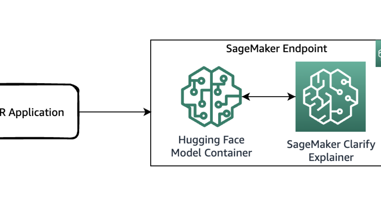
The following diagram shows the SageMaker architecture for hosting an endpoint that serves explainability requests. It includes interactions between an endpoint, the model container, and the SageMaker Clarify explainer.
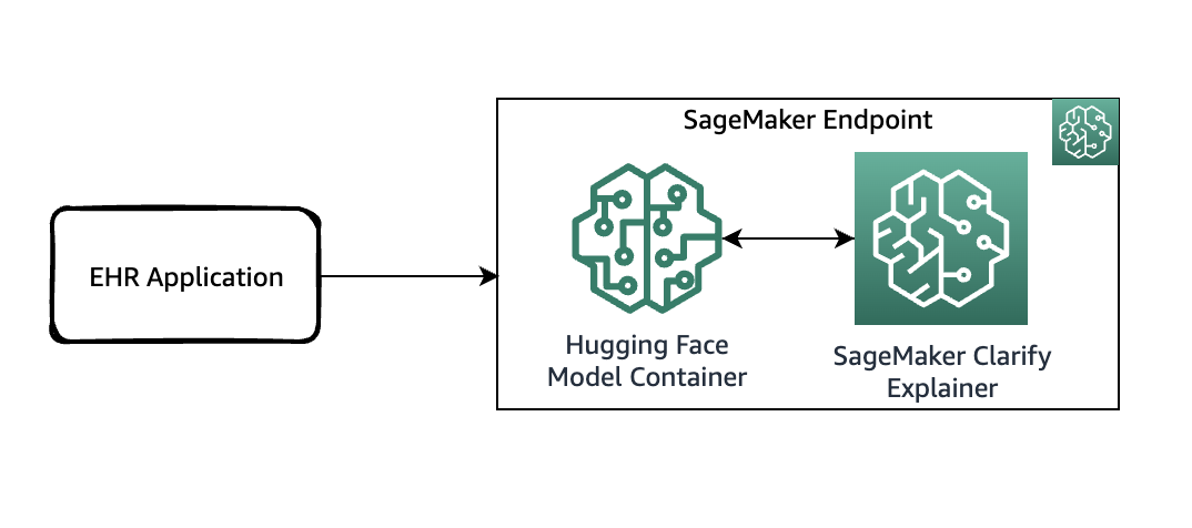
In the sample code, we use a Jupyter notebook to showcase the functionality. However, in a real-world use case, electronic health records (EHRs) or other hospital care applications would directly invoke the SageMaker endpoint to get the same response. In the Jupyter notebook, we deploy a Hugging Face model container to a SageMaker endpoint. Then we use SageMaker Clarify to explain the results that we obtain from the deployed model.
Prerequisites
You need the following prerequisites:
Access the code from the GitHub repository and upload it to your notebook instance. You can also run the notebook in an Amazon SageMaker Studio environment, which is an integrated development environment (IDE) for ML development. We recommend using a Python 3 (Data Science) kernel on SageMaker Studio or a conda_python3 kernel on a SageMaker notebook instance.
Deploy the model with SageMaker Clarify enabled
As the first step, download the model from Hugging Face and upload it to an Amazon Simple Storage Service (Amazon S3) bucket. Then create a model object using the HuggingFaceModel class. This uses a prebuilt container to simplify the process of deploying Hugging Face models to SageMaker. You also use a custom inference script to do the predictions within the container. The following code illustrates the script that is passed as an argument to the HuggingFaceModel class:
Then you can define the instance type that you deploy this model on:
We then populate ExecutionRoleArn, ModelName and PrimaryContainer fields to create a Model.
Next, create an endpoint configuration by calling the create_endpoint_config API. Here, you supply the same model_name used in the create_model API call. The create_endpoint_config now supports the additional parameter ClarifyExplainerConfig to enable the SageMaker Clarify explainer. The SHAP baseline is mandatory; you can provide it either as inline baseline data (the ShapBaseline parameter) or by a S3 baseline file (the ShapBaselineUri parameter). For optional parameters, see the developer guide.
In the following code, we use a special token as the baseline:
The TextConfig is configured with sentence-level granularity (each sentence is a feature, and we need a few sentences per review for good visualization) and the language as English:
Finally, after you have the model and endpoint configuration ready, use the create_endpoint API to create your endpoint. The endpoint_name must be unique within a Region in your AWS account. The create_endpoint API is synchronous in nature and returns an immediate response with the endpoint status being in the Creating state.
Explain the prediction
Now that you have deployed the endpoint with online explainability enabled, you can try some examples. You can invoke the real-time endpoint using the invoke_endpoint method by providing the serialized payload, which in this case is some sample admission notes:
In the first scenario, let’s assume that the following medical admission note was taken by a healthcare worker:
The following screenshot shows the model results.
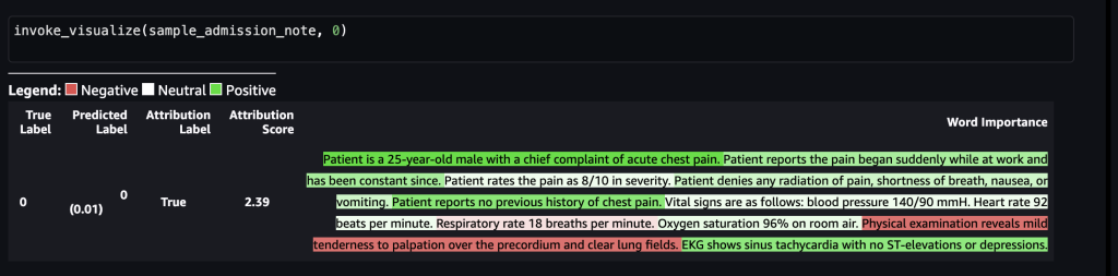
After this is forwarded to the SageMaker endpoint, the label was predicted as 0, which indicates that the risk of mortality is low. In other words, 0 implies that the admitted patient is in non-acute condition according to the model. However, we need the reasoning behind that prediction. For that, you can use the SHAP values as the response. The response includes the SHAP values corresponding to the phrases of the input note, which can be further color-coded as green or red based on how the SHAP values contribute to the prediction. In this case, we see more phrases in green, such as “Patient reports no previous history of chest pain” and “EKG shows sinus tachycardia with no ST-elevations or depressions,” as opposed to red, aligning with the mortality prediction of 0.
In the second scenario, let’s assume that the following medical admission note was taken by a healthcare worker:
The following screenshot shows our results.
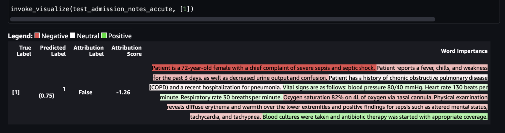
After this is forwarded to the SageMaker endpoint, the label was predicted as 1, which indicates that the risk of mortality is high. This implies that the admitted patient is in acute condition according to the model. However, we need the reasoning behind that prediction. Again, you can use the SHAP values as the response. The response includes the SHAP values corresponding to the phrases of the input note, which can be further color-coded. In this case, we see more phrases in red, such as “Patient reports a fever, chills, and weakness for the past 3 days, as well as decreased urine output and confusion” and “Patient is a 72-year-old female with a chief complaint of severe sepsis shock,” as opposed to green, aligning with the mortality prediction of 1.
The clinical care team can use these explanations to assist in their decisions on the care process for each individual patient.
Clean up
To clean up the resources that have been created as part of this solution, run the following statements:
Conclusion
This post showed you how to use SageMaker Clarify to explain decisions in a healthcare use case based on the medical notes captured during various stages of triage process. This solution can be integrated into existing decision support systems to provide another data point to clinicians as they evaluate patients for admission into the ICU. To learn more about using AWS services in the healthcare industry, check out the following blog posts:
- Introducing the Healthcare Industry Lens for the AWS Well-Architected Framework
- How Telescope Health Streamlines Virtual Care in the Cloud
- The Pathway to better Surgical Care with Operating Room Analytics on AWS
- Predicting diabetic patient readmission using multi-model training on Amazon SageMaker Pipelines
- How Pieces Technologies leverages AWS services to predict patient outcomes
References
[1] https://aclanthology.org/2021.eacl-main.75/ [2] https://arxiv.org/pdf/1705.07874.pdfAbout the authors
 Shamika Ariyawansa, serving as a Senior AI/ML Solutions Architect in the Global Healthcare and Life Sciences division at Amazon Web Services (AWS), has a keen focus on Generative AI. He assists customers in integrating Generative AI into their projects, emphasizing the importance of explainability within their AI-driven initiatives. Beyond his professional commitments, Shamika passionately pursues skiing and off-roading adventures.”
 Ted Spencer is an experienced Solutions Architect with extensive acute healthcare experience. He is passionate about applying machine learning to solve new use cases, and rounds out solutions with both the end consumer and their business/clinical context in mind. He lives in Toronto Ontario, Canada, and enjoys traveling with his family and training for triathlons as time permits.
 Ram Pathangi is a Solutions Architect at AWS supporting healthcare and life sciences customers in the San Francisco Bay Area. He has helped customers in finance, healthcare, life sciences, and hi-tech verticals run their business successfully on the AWS Cloud. He specializes in Databases, Analytics, and Machine Learning.
Apply fine-grained data access controls with AWS Lake Formation in Amazon SageMaker Data Wrangler
Amazon SageMaker Data Wrangler reduces the time it takes to collect and prepare data for machine learning (ML) from weeks to minutes. You can streamline the process of feature engineering and data preparation with SageMaker Data Wrangler and finish each stage of the data preparation workflow (including data selection, purification, exploration, visualization, and processing at scale) within a single visual interface. Data is frequently kept in data lakes that can be managed by AWS Lake Formation, giving you the ability to implement fine-grained access control using a straightforward grant or revoke procedure. SageMaker Data Wrangler supports fine-grained data access control with Lake Formation and Amazon Athena connections.
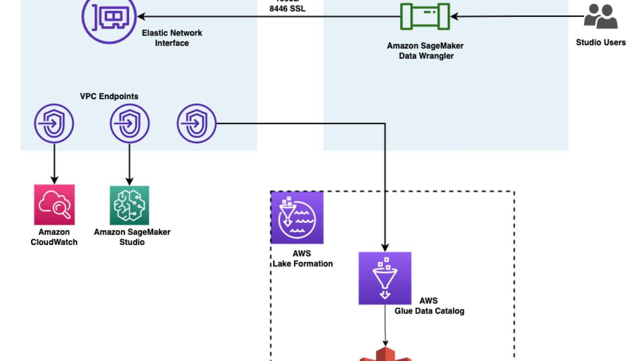
We are happy to announce that SageMaker Data Wrangler now supports using Lake Formation with Amazon EMR to provide this fine-grained data access restriction.
Data professionals such as data scientists want to use the power of Apache Spark, Hive, and Presto running on Amazon EMR for fast data preparation; however, the learning curve is steep. Our customers wanted the ability to connect to Amazon EMR to run ad hoc SQL queries on Hive or Presto to query data in the internal metastore or external metastore (such as the AWS Glue Data Catalog), and prepare data within a few clicks.
In this post, we show how to use Lake Formation as a central data governance capability and Amazon EMR as a big data query engine to enable access for SageMaker Data Wrangler. The capabilities of Lake Formation simplify securing and managing distributed data lakes across multiple accounts through a centralized approach, providing fine-grained access control.
Solution overview
We demonstrate this solution with an end-to-end use case using a sample dataset, the TPC data model. This data represents transaction data for products and includes information such as customer demographics, inventory, web sales, and promotions. To demonstrate fine-grained data access permissions, we consider the following two users:
- David, a data scientist on the marketing team. He is tasked with building a model on customer segmentation, and is only permitted to access non-sensitive customer data.
- Tina, a data scientist on the sales team. She is tasked with building the sales forecast model, and needs access to sales data for the particular region. She is also helping the product team with innovation, and therefore needs access to product data as well.
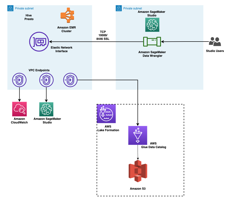
The architecture is implemented as follows:
- Lake Formation manages the data lake, and the raw data is available in Amazon Simple Storage Service (Amazon S3) buckets
- Amazon EMR is used to query the data from the data lake and perform data preparation using Spark
- AWS Identity and Access Management (IAM) roles are used to manage data access using Lake Formation
- SageMaker Data Wrangler is used as the single visual interface to interactively query and prepare the data
The following diagram illustrates this architecture. Account A is the data lake account that houses all the ML-ready data obtained through extract, transform, and load (ETL) processes. Account B is the data science account where a group of data scientists compile and run data transformations using SageMaker Data Wrangler. In order for SageMaker Data Wrangler in Account B to have access to the data tables in Account A’s data lake via Lake Formation permissions, we must activate the necessary rights.
You can use the provided AWS CloudFormation stack to set up the architectural components for this solution.
Prerequisites
Before you get started, make sure you have the following prerequisites:
- An AWS account
- An IAM user with administrator access
- An S3 bucket
Provision resources with AWS CloudFormation
We provide a CloudFormation template that deploys the services in the architecture for end-to-end testing and to facilitate repeated deployments. The outputs of this template are as follows:
- An S3 bucket for the data lake.
- An EMR cluster with EMR runtime roles enabled. For more details on using runtime roles with Amazon EMR, see Configure runtime roles for Amazon EMR steps. Associating runtime roles with EMR clusters is supported in Amazon EMR 6.9. Make sure the following configuration is in place:
- Create a security configuration in Amazon EMR.
- The EMR runtime role’s trust policy should allow the EMR EC2 instance profile to assume the role.
- The EMR EC2 instance profile role should be able to assume the EMR runtime roles.
- The EMR cluster should be created with encryption in transit.
- IAM roles for accessing the data in data lake, with fine-grained permissions:
- Marketing-data-access-role
- Sales-data-access-role
- An Amazon SageMaker Studio domain and two user profiles. The SageMaker Studio execution roles for the users allow the users to assume their corresponding EMR runtime roles.
- A lifecycle configuration to enable the selection of the role to use for the EMR connection.
- A Lake Formation database populated with the TPC data.
- Networking resources required for the setup, such as VPC, subnets, and security groups.
Create Amazon EMR encryption certificates for the data in transit
With Amazon EMR release version 4.8.0 or later, you have option for specifying artifacts for encrypting data in transit using a security configuration. We manually create PEM certificates, include them in a .zip file, upload it to an S3 bucket, and then reference the .zip file in Amazon S3. You likely want to configure the private key PEM file to be a wildcard certificate that enables access to the VPC domain in which your cluster instances reside. For example, if your cluster resides in the us-east-1 Region, you could specify a common name in the certificate configuration that allows access to the cluster by specifying CN=*.ec2.internal in the certificate subject definition. If your cluster resides in us-west-2, you could specify CN=*.us-west-2.compute.internal.
Run the following commands using your system terminal. This will generate PEM certificates and collate them into a .zip file:
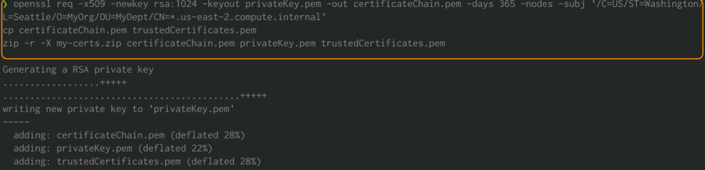
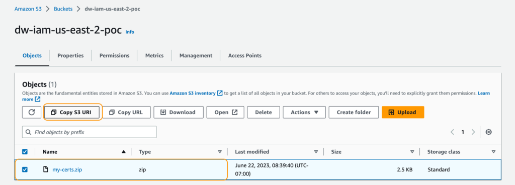
Upload my-certs.zip to an S3 bucket in the same Region where you intend to run this exercise. Copy the S3 URI for the uploaded file. You’ll need this while launching the CloudFormation template.
This example is a proof of concept demonstration only. Using self-signed certificates is not recommended and presents a potential security risk. For production systems, use a trusted certification authority (CA) to issue certificates.
Deploying the CloudFormation template
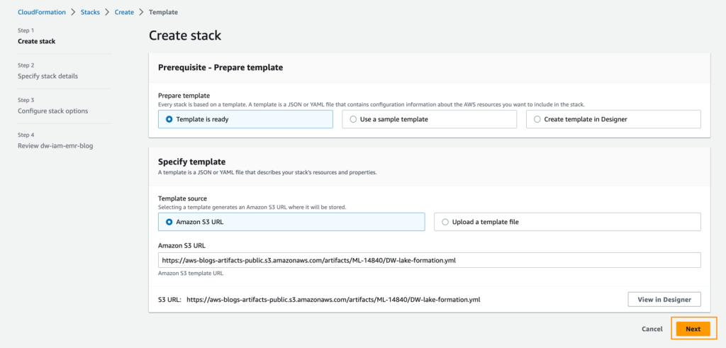
To deploy the solution, complete the following steps:
- Sign in to the AWS Management Console as an IAM user, preferably an admin user.
- Choose Launch Stack to launch the CloudFormation template:
![]()
- Choose Next.
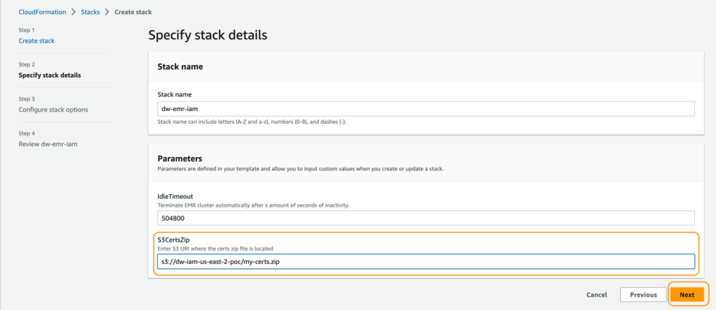
- For Stack name, enter a name for the stack.
- For IdleTimeout, enter a value for the idle timeout for the EMR cluster (to avoid paying for the cluster when it’s not being used).
- For S3CertsZip, enter an S3 URI with the EMR encryption key.
For instructions to generate a key and .zip file specific to your Region, refer to Providing certificates for encrypting data in transit with Amazon EMR encryption. If you are deploying in US East (N. Virginia), remember to use CN=*.ec2.internal. For more information, refer to Create keys and certificates for data encryption. Make sure to upload the .zip file to an S3 bucket in the same Region as your CloudFormation stack deployment.
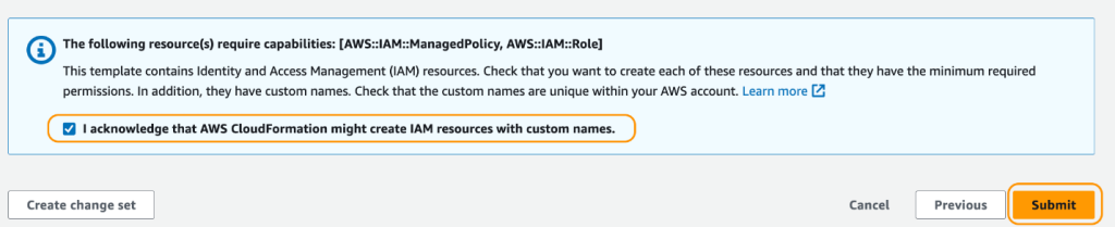
- On the review page, select the check box to confirm that AWS CloudFormation might create resources.
- Choose Create stack.
Wait until the status of the stack changes from CREATE_IN_PROGRESS to CREATE_COMPLETE. The process usually takes 10–15 minutes.
After the stack is created, allow Amazon EMR to query Lake Formation by updating the External Data Filtering settings on Lake Formation. For instructions, refer to Getting started with Lake Formation. Specify Amazon EMR for Session tag values and enter your AWS account ID under AWS account IDs.
Test data access permissions
Now that the necessary infrastructure is in place, you can verify that the two SageMaker Studio users have access to granular data. To review, David shouldn’t have access to any private information about your customers. Tina has access to information about sales. Let’s put each user type to the test.
Test David’s user profile
To test your data access with David’s user profile, complete the following steps:
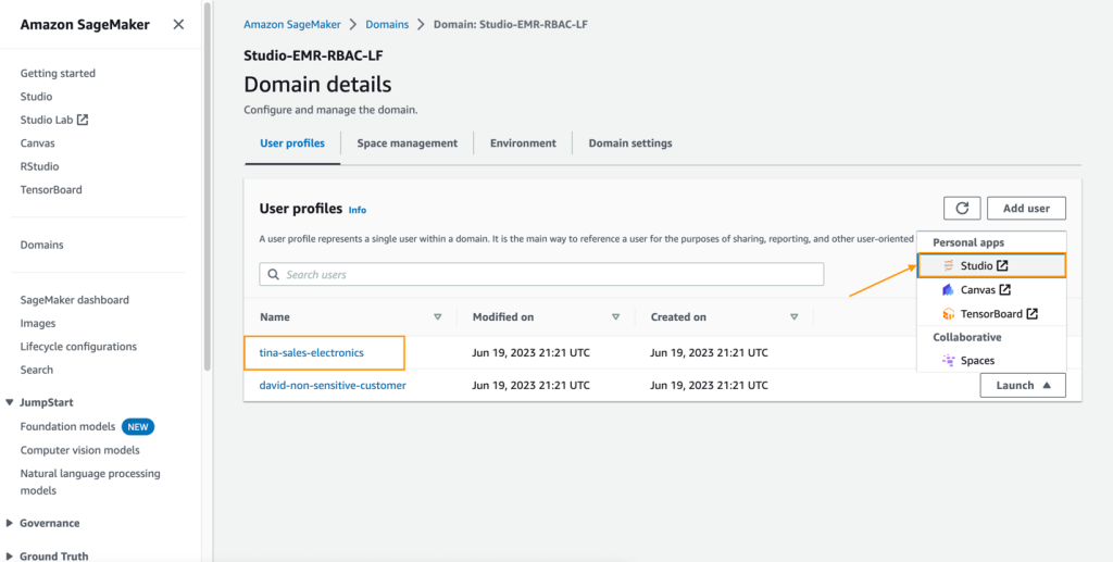
- On the SageMaker console, choose Domains in the navigation pane.
- From the SageMaker Studio domain, launch SageMaker Studio from the user profile david-non-sensitive-customer.
- In your SageMaker Studio environment, create an Amazon SageMaker Data Wrangler flow, and choose Import & prepare data visually.
Alternatively, on the File menu, choose New, then choose Data Wrangler flow.
We discuss these steps to create a data flow in detail later in this post.
Test Tina’s user profile
Tina’s SageMaker Studio execution role allows her to access the Lake Formation database using two EMR execution roles. This is achieved by listing the role ARNs in a configuration file in Tina’s file directory. These roles can be set using SageMaker Studio lifecycle configurations to persist the roles across app restarts. To test Tina’s access, complete the following steps:
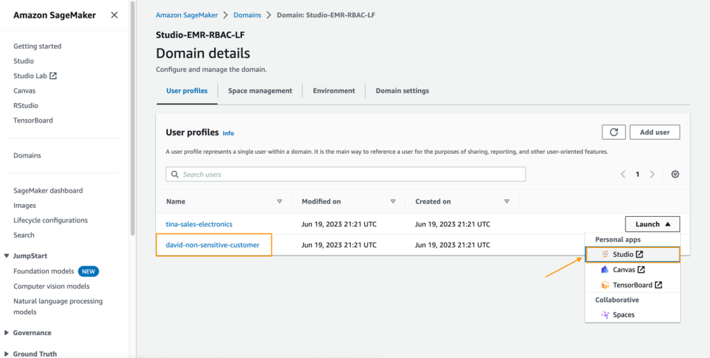
- On the SageMaker console, navigate to the SageMaker Studio domain.
- Launch SageMaker Studio from the user profile
tina-sales-electronics.
It’s a good practice to close any previous SageMaker Studio sessions on your browser when switching user profiles. There can only be one active SageMaker Studio user session at a time.
- Create a Data Wrangler data flow.
In the following sections, we showcase creating a data flow within SageMaker Data Wrangler and connecting to Amazon EMR as the data source. David and Tina will have similar experiences with data preparation, except for access permissions, so they will see different tables.
Create a SageMaker Data Wrangler data flow
In this section, we cover connecting to the existing EMR cluster created through the CloudFormation template as a data source in SageMaker Data Wrangler. For demonstration purposes, we use David’s user profile.
To create your data flow, complete the following steps:
- On the SageMaker console, choose Domains in the navigation pane.
- Choose StudioDomain, which was created by running the CloudFormation template.
- Select a user profile (for this example, David’s) and launch SageMaker Studio.
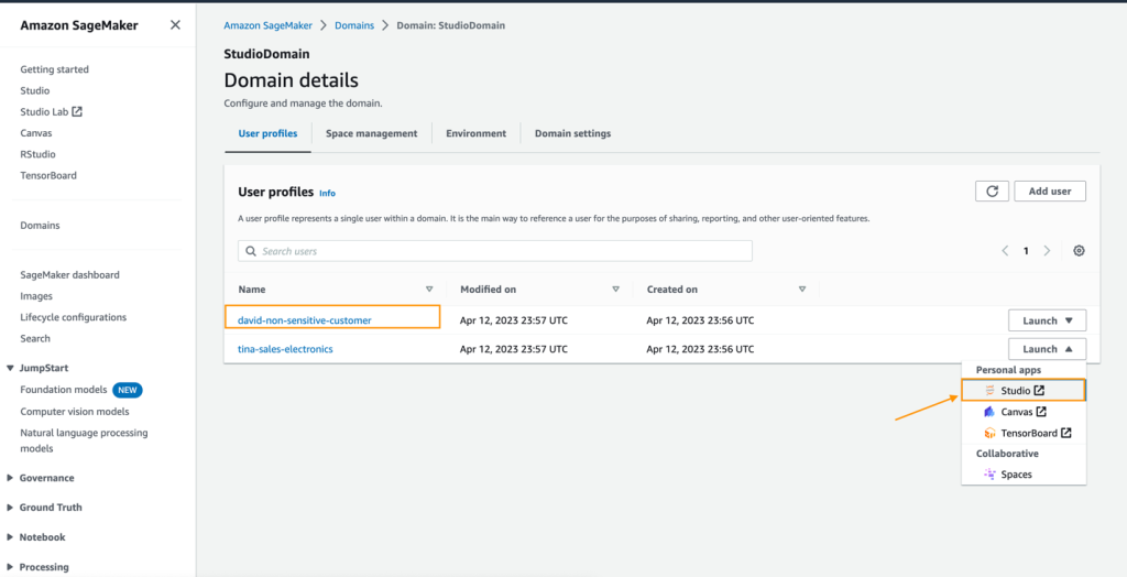
- Choose Open Studio.
- In SageMaker Studio, create a new data flow and choose Import & prepare data visually.
Alternatively, on the File menu, choose New, then choose Data Wrangler flow.
Creating a new flow can take a few minutes. After the flow has been created, you see the Import data page.
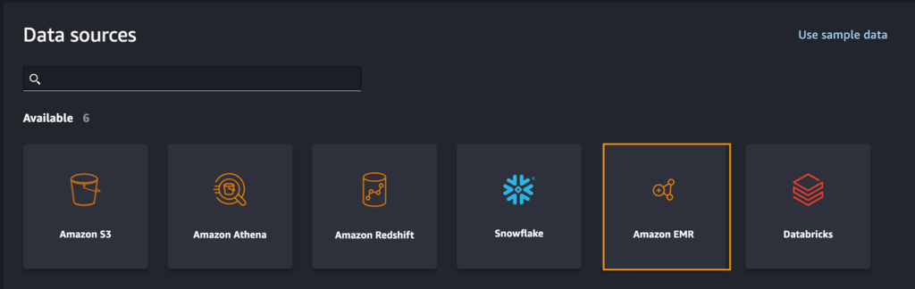
- To add Amazon EMR as a data source in SageMaker Data Wrangler, on the Add data source menu, choose Amazon EMR.
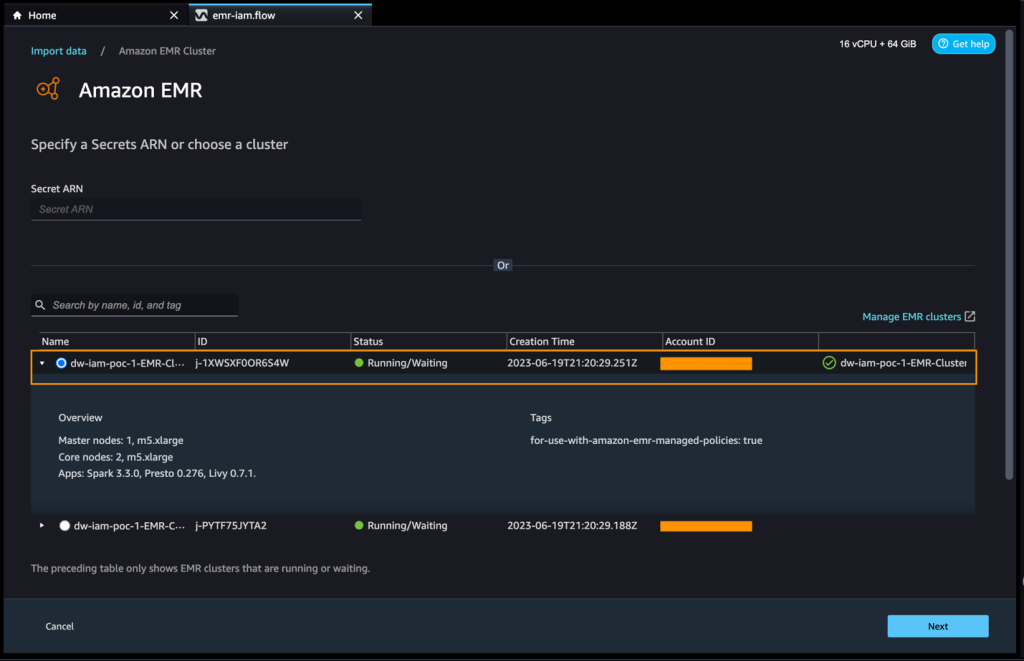
You can browse all the EMR clusters that your SageMaker Studio execution role has permissions to see. You have two options to connect to a cluster: one is through the interactive UI, and the other is to first create a secret using AWS Secrets Manager with a JDBC URL, including EMR cluster information, and then provide the stored AWS secret ARN in the UI to connect to Presto or Hive. In this post, we use the first method.
- Select any of the clusters that you want to use, then choose Next.
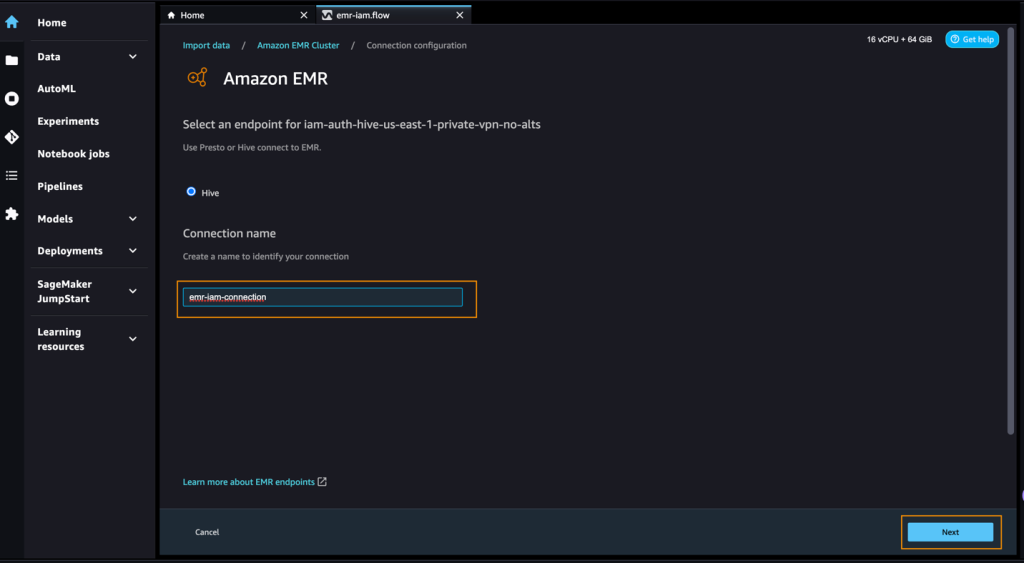
- Select which endpoint you want to use.
- Enter a name to identify your connection, such as
emr-iam-connection, then choose Next.
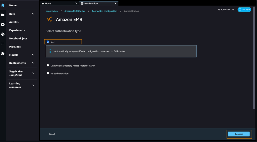
- Select IAM as your authentication type and choose Connect.
When you’re connected, you can interactively view a database tree and table preview or schema. You can also query, explore, and visualize data from Amazon EMR. For a preview, you see a limit of 100 records by default. After you provide a SQL statement in the query editor and choose Run, the query is run on the Amazon EMR Hive engine to preview the data. Choose Cancel query to cancel ongoing queries if they are taking an unusually long time.
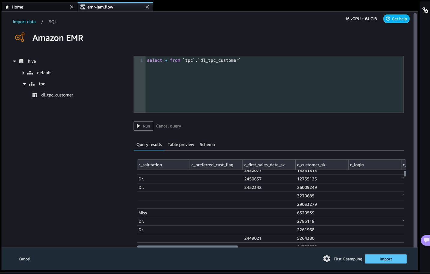
- Let’s access data from the table that David doesn’t have permissions to.
The query will result in the error message “Unable to fetch table dl_tpc_web_sales. Insufficient Lake Formation permission(s) on dl_tpc_web_sales.”
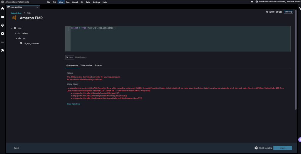
The last step is to import the data. When you are ready with the queried data, you have the option to update the sampling settings for the data selection according to the sampling type (FirstK, Random, or Stratified) and the sampling size for importing data into Data Wrangler.
- Choose Import to import the data.
On the next page, you can add various transformations and essential analysis to the dataset.
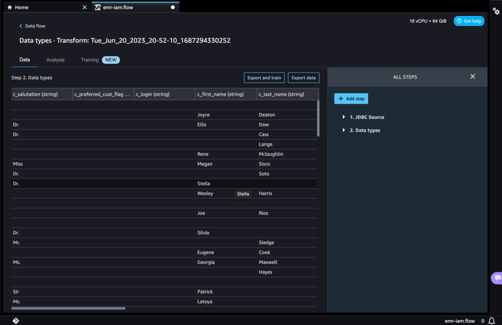
- Navigate to the data flow and add more steps to the flow as needed for transformations and analysis.
You can run a data insight report to identify data quality issues and get recommendations to fix those issues. Let’s look at some example transforms.
- In the Data flow view, you should see that we are using Amazon EMR as a data source using the Hive connector.
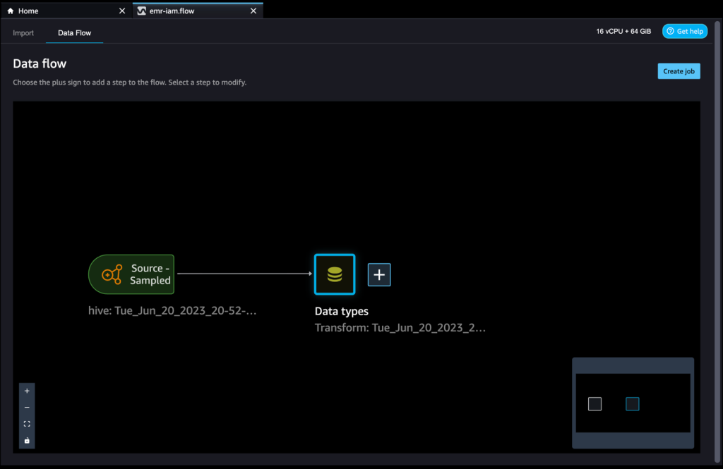
- Choose the plus sign next to Data types and choose Add transform.
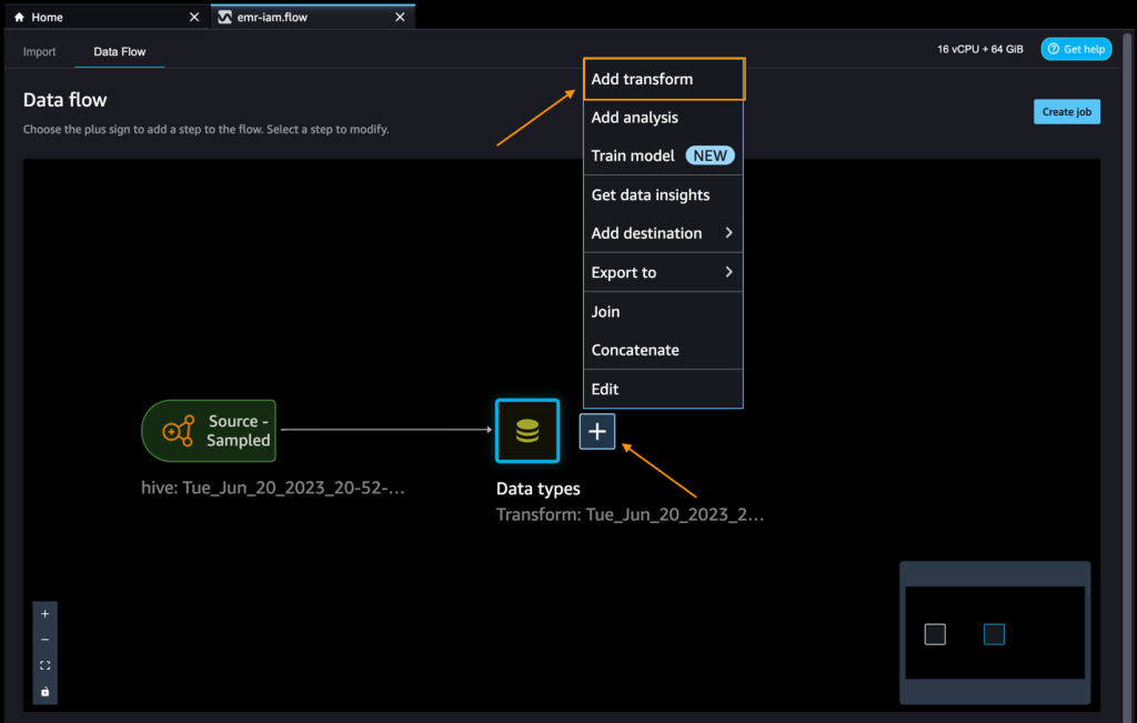
Let’s explore the data and apply a transformation. For example, the c_login column is empty and it will not add value as a feature. Let’s delete the column.
- In the All steps pane, choose Add step.
- Choose Manage columns.
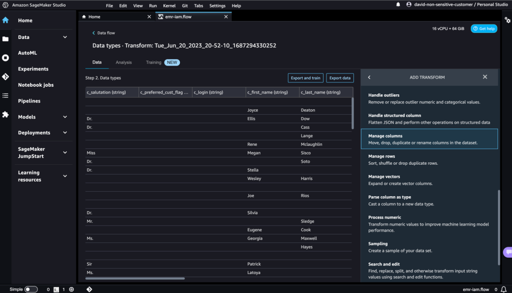
- For Transform, choose Drop column.
- For Columns to drop, choose the
c_logincolumn. - Choose Preview, then choose Add.
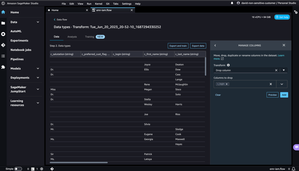
- Verify the step by expanding the Drop column section.
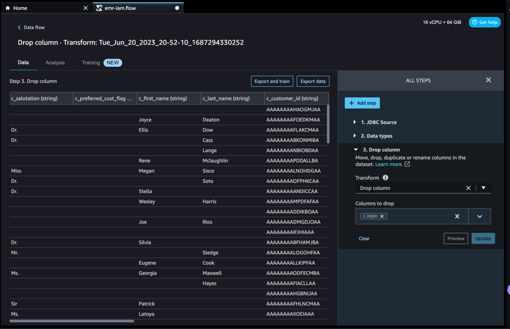
You can continue adding steps based on the different transformations required for your dataset. Let’s go back to our data flow. You can now see the Drop column block showing the transform we performed.
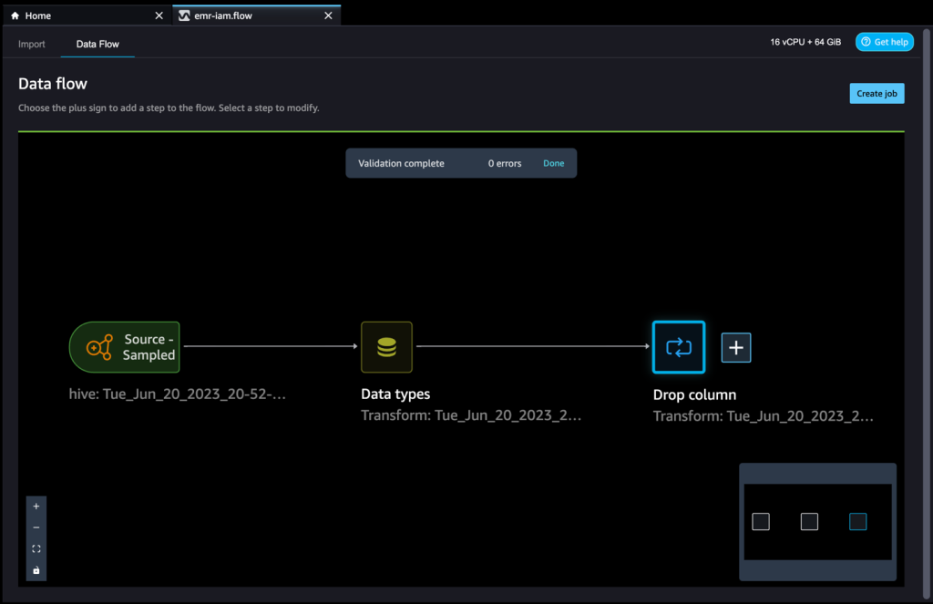
ML practitioners spend a lot of time crafting feature engineering code, applying it to their initial datasets, training models on the engineered datasets, and evaluating model accuracy. Given the experimental nature of this work, even the smallest project will lead to multiple iterations. The same feature engineering code is often run again and again, wasting time and compute resources on repeating the same operations. In large organizations, this can cause an even greater loss of productivity because different teams often run identical jobs or even write duplicate feature engineering code because they have no knowledge of prior work. To avoid the reprocessing of features, we can export our transformed features to Amazon SageMaker Feature Store. For more information, refer to New – Store, Discover, and Share Machine Learning Features with Amazon SageMaker Feature Store.
- Choose the plus sign next to Drop column.
- Choose Export to and SageMaker Feature Store (via Jupyter notebook).
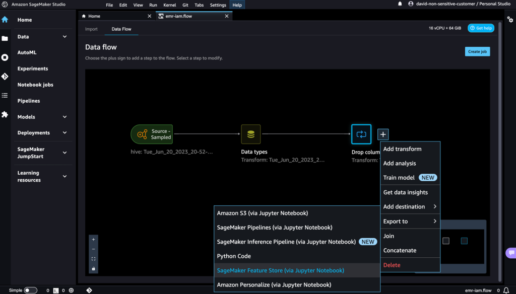
You can easily export your generated features to SageMaker Feature Store by specifying it as the destination. You can save the features into an existing feature group or create a new one. For more information, refer to Easily create and store features in Amazon SageMaker without code.
We have now created features with SageMaker Data Wrangler and stored those features in SageMaker Feature Store. We showed an example workflow for feature engineering in the SageMaker Data Wrangler UI.
Clean up
If your work with SageMaker Data Wrangler is complete, delete the resources you created to avoid incurring additional fees.
- In SageMaker Studio, close all the tabs, then on the File menu, choose Shut Down.
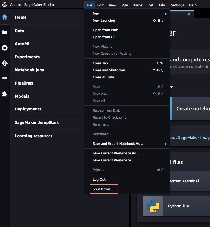
- When prompted, choose Shutdown All.
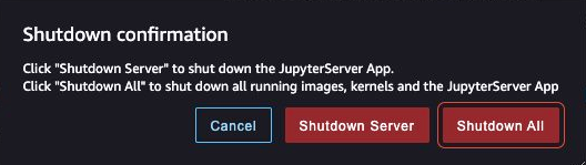
Shutdown might take a few minutes based on the instance type. Make sure all the apps associated with each user profile got deleted. If they were not deleted, manually delete the app associated under each user profile created using the CloudFormation template.
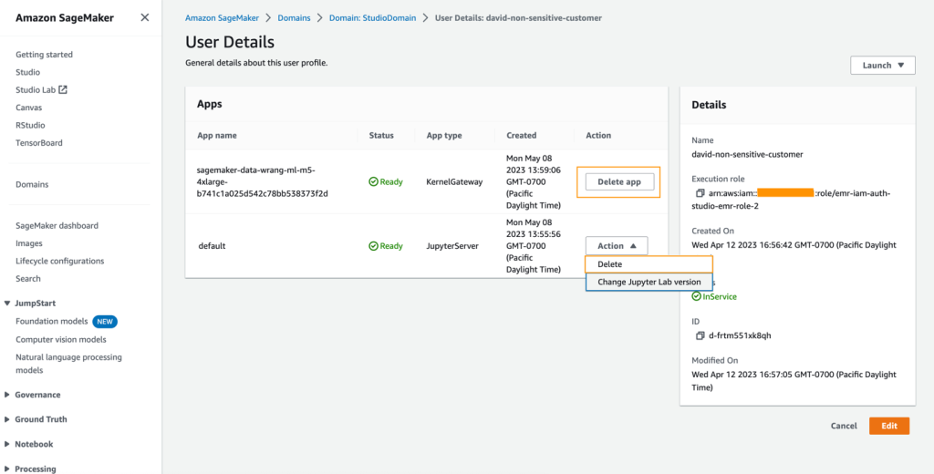
- On the Amazon S3 console, empty any S3 buckets that were created from the CloudFormation template when provisioning clusters.
The buckets should have the same prefix as the CloudFormation launch stack name and cf-templates-.
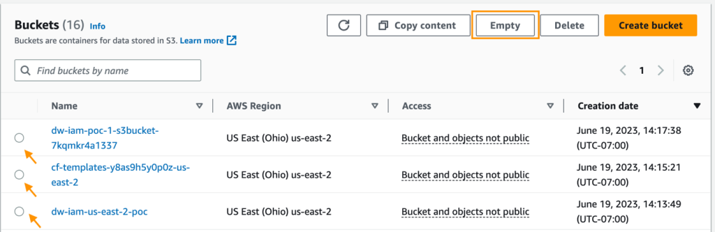
- On the Amazon EFS console, delete the SageMaker Studio file system.
You can confirm that you have the correct file system by choosing the file system ID and confirming the tag ManagedByAmazonSageMakerResource on the Tags tab.
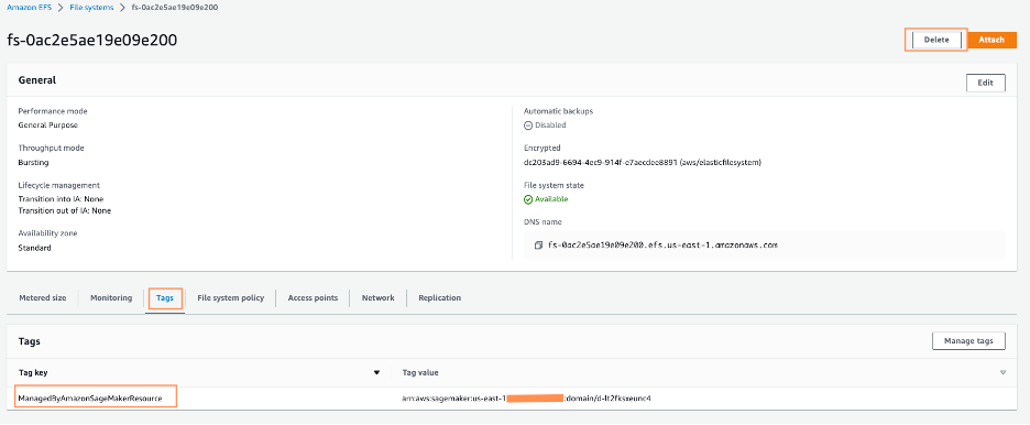
- On the AWS CloudFormation console, select the stack you created and choose Delete.
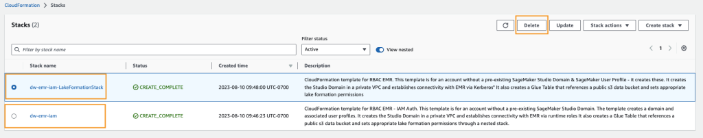
You’ll receive an error message, which is expected. We’ll come back to this and clean it up in the subsequent steps.
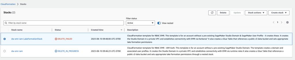
- Identify the VPC that was created by the CloudFormation stack, named dw-emr-, and follow the prompts to delete the VPC.
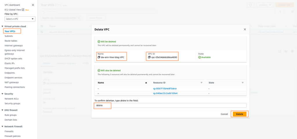
- Return to the AWS CloudFormation console and retry the stack deletion for dw-emr-.
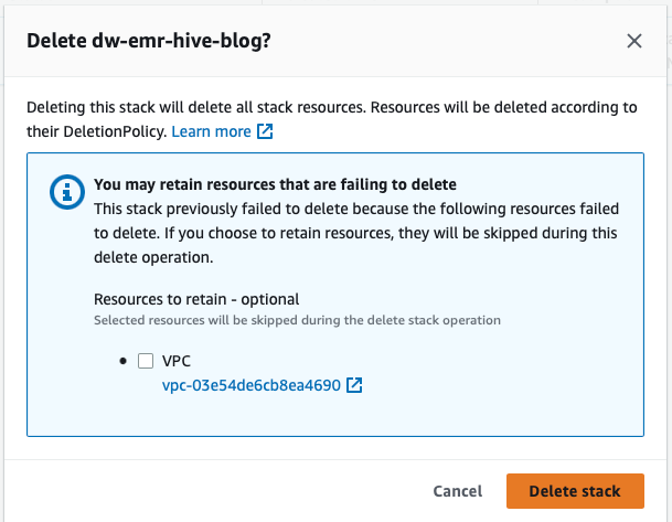
All the resources provisioned by the CloudFormation template described in this post have now been removed from your account.
Conclusion
In this post, we went over how to apply fine-grained access control with Lake Formation and access the data using Amazon EMR as a data source in SageMaker Data Wrangler, how to transform and analyze a dataset, and how to export the results to a data flow for use in a Jupyter notebook. After visualizing our dataset using SageMaker Data Wrangler’s built-in analytical features, we further enhanced our data flow. The fact that we created a data preparation pipeline without writing a single line of code is significant.
To get started with SageMaker Data Wrangler, refer to Prepare ML Data with Amazon SageMaker Data Wrangler.
About the Authors
 Ajjay Govindaram is a Senior Solutions Architect at AWS. He works with strategic customers who are using AI/ML to solve complex business problems. His experience lies in providing technical direction as well as design assistance for modest to large-scale AI/ML application deployments. His knowledge ranges from application architecture to big data, analytics, and machine learning. He enjoys listening to music while resting, experiencing the outdoors, and spending time with his loved ones.
 Isha Dua is a Senior Solutions Architect based in the San Francisco Bay Area. She helps AWS enterprise customers grow by understanding their goals and challenges, and guides them on how they can architect their applications in a cloud-native manner while ensuring resilience and scalability. She’s passionate about machine learning technologies and environmental sustainability.
 Parth Patel is a Senior Solutions Architect at AWS in the San Francisco Bay Area. Parth guides enterprise customers to accelerate their journey to the cloud and help them adopt and grow on the AWS Cloud successfully. He is passionate about machine learning technologies, environmental sustainability, and application modernization.