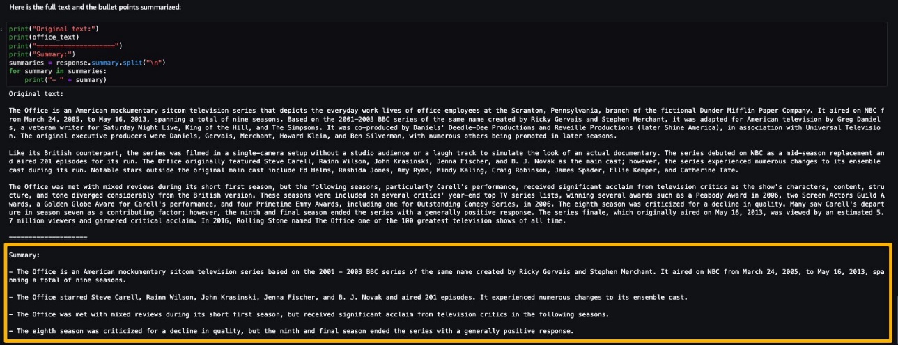
Cost of poor quality is top of mind for manufacturers. Quality defects increase scrap and rework costs, decrease throughput, and can impact customers and company reputation. Quality inspection on the production line is crucial for maintaining quality standards. In many cases, human visual inspection is used to assess the quality and detect defects, which can limit the throughput of the line due to limitations of human inspectors.
The advent of machine learning (ML) and artificial intelligence (AI) brings additional visual inspection capabilities using computer vision (CV) ML models. Complimenting human inspection with CV-based ML can reduce detection errors, speed up production, reduce the cost of quality, and positively impact customers. Building CV ML models typically requires expertise in data science and coding, which are often rare resources in manufacturing organizations. Now, quality engineers and others on the shop floor can build and evaluate these models using no-code ML services, which can accelerate exploration and adoption of these models more broadly in manufacturing operations.
Amazon SageMaker Canvas is a visual interface that enables quality, process, and production engineers to generate accurate ML predictions on their own—without requiring any ML experience or having to write a single line of code. You can use SageMaker Canvas to create single-label image classification models for identifying common manufacturing defects using your own image datasets.
In this post, you will learn how to use SageMaker Canvas to build a single-label image classification model to identify defects in manufactured magnetic tiles based on their image.
Solution overview
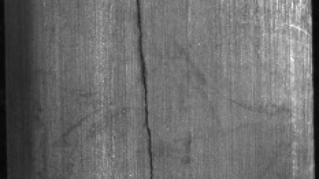
This post assumes the viewpoint of a quality engineer exploring CV ML inspection, and you will work with sample data of magnetic tile images to build an image classification ML model to predict defects in the tiles for the quality check. The dataset contains more than 1,200 images of magnetic tiles, which have defects such as blowhole, break, crack, fray, and uneven surface. The following images provide an example of single-label defect classification, with a cracked tile on the left and a tile free of defects on the right.
 |
 |
In a real-world example, you can collect such images from the finished products in the production line. In this post, you use SageMaker Canvas to build a single-label image classification model that will predict and classify defects for a given magnetic tile image.
SageMaker Canvas can import image data from a local disk file or Amazon Simple Storage Service (Amazon S3). For this post, multiple folders have been created (one per defect type such as blowhole, break, or crack) in an S3 bucket, and magnetic tile images are uploaded to their respective folders. The folder called Free contains defect-free images.

There are four steps involved in building the ML model using SageMaker Canvas:
- Import the dataset of the images.
- Build and train the model.
- Analyze the model insights, such as accuracy.
- Make predictions.
Prerequisites
Before starting, you need to set up and launch SageMaker Canvas. This setup is performed by an IT administrator and involves three steps:
- Set up an Amazon SageMaker domain.
- Set up the users.
- Set up permissions to use specific features in SageMaker Canvas.
Refer to Getting started with using Amazon SageMaker Canvas and Setting Up and Managing Amazon SageMaker Canvas (for IT Administrators) to configure SageMaker Canvas for your organization.
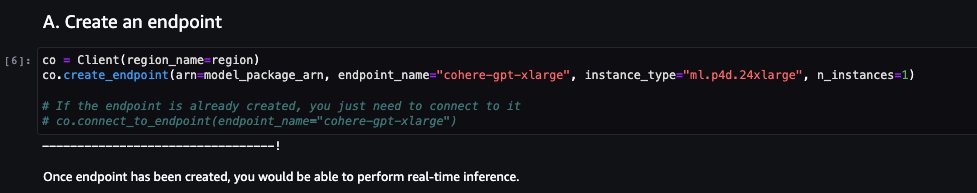
When SageMaker Canvas is set up, the user can navigate to the SageMaker console, choose Canvas in the navigation pane, and choose Open Canvas to launch SageMaker Canvas.

The SageMaker Canvas application is launched in a new browser window.

After the SageMaker Canvas application is launched, you start the steps of building the ML model.
Import the dataset
Importing the dataset is the first step when building an ML model with SageMaker Canvas.
- In the SageMaker Canvas application, choose Datasets in the navigation pane.
- On the Create menu, choose Image.

- For Dataset name, enter a name, such as
Magnetic-Tiles-Dataset. - Choose Create to create the dataset.

After the dataset is created, you need to import images in the dataset.
- On the Import page, choose Amazon S3 (the magnetic tiles images are in an S3 bucket).
You have the choice to upload the images from your local computer as well.

- Select the folder in the S3 bucket where the magnetic tile images are stored and chose Import Data.

SageMaker Canvas starts importing the images into the dataset. When the import is complete, you can see the image dataset created with 1,266 images.

You can choose the dataset to check the details, such as a preview of the images and their label for the defect type. Because the images were organized in folders and each folder was named with the defect type, SageMaker Canvas automatically completed the labeling of the images based on the folder names. As an alternative, you can import unlabeled images, add labels, and perform labeling of the individual images at a later point of time. You can also modify the labels of the existing labeled images.

The image import is complete and you now have an images dataset created in the SageMaker Canvas. You can move to the next step to build an ML model to predict defects in the magnetic tiles.
Build and train the model
You train the model using the imported dataset.
- Choose the dataset (
Magnetic-tiles-Dataset) and choose Create a model. - For Model name, enter a name, such as
Magnetic-Tiles-Defect-Model. - Select Image analysis for the problem type and choose Create to configure the model build.

On the model’s Build tab, you can see various details about the dataset, such as label distribution, count of labeled vs. unlabeled images, and also model type, which is single-label image prediction in this case. If you have imported unlabeled images or you want to modify or correct the labels of certain images, you can choose Edit dataset to modify the labels.

You can build model in two ways: Quick build and Standard build. The Quick build option prioritizes speed over accuracy. It trains the model in 15–30 minutes. The model can be used for the prediction but it can’t be shared. It’s a good option to quickly check feasibility and accuracy of training a model with a given dataset. The Standard build chooses accuracy over speed, and model training can take between 2–4 hours.
For this post, you train the model using the Standard build option.
- Choose Standard build on the Build tab to start training the model.

The model training starts instantly. You can see the expected build time and training progress on the Analyze tab.

Wait until the model training is complete, then you can analyze model performance for the accuracy.
Analyze the model
In this case, it took less than an hour to complete the model training. When the model training is complete, you can check model accuracy on the Analyze tab to determine if the model can accurately predict defects. You see the overall model accuracy is 97.7% in this case. You can also check the model accuracy for each of the individual label or defect type, for instance 100% for Fray and Uneven but approximately 95% for Blowhole. This level of accuracy is encouraging, so we can continue the evaluation.

To better understand and trust the model, enable Heatmap to see the areas of interest in the image that the model uses to differentiate the labels. It’s based on the class activation map (CAM) technique. You can use the heatmap to identify patterns from your incorrectly predicted images, which can help improve the quality of your model.

On the Scoring tab, you can check precision and recall for the model for each of the labels (or class or defect type). Precision and recall are evaluation metrics used to measure the performance of a binary and multiclass classification model. Precision tells how good the model is at predicting a specific class (defect type, in this example). Recall tells how many times the model was able to detect a specific class.

Model analysis helps you understand the accuracy of the model before you use it for prediction.
Make predictions
After the model analysis, you can now make predictions using this model to identify defects in the magnetic tiles.
On the Predict tab, you can choose Single prediction and Batch prediction. In a single prediction, you import a single image from your local computer or S3 bucket to make a prediction about the defect. In batch prediction, you can make predictions for multiple images that are stored in a SageMaker Canvas dataset. You can create a separate dataset in SageMaker Canvas with the test or inference images for the batch prediction. For this post, we use both single and batch prediction.
For single prediction, on the Predict tab, choose Single prediction, then choose Import image to upload the test or inference image from your local computer.

After the image is imported, the model makes a prediction about the defect. For the first inference, it might take few minutes because the model is loading for the first time. But after the model is loaded, it makes instant predictions about the images. You can see the image and the confidence level of the prediction for each label type. For instance, in this case, the magnetic tile image is predicted to have an uneven surface defect (the Uneven label) and the model is 94% confident about it.

Similarly, you can use other images or a dataset of images to make predictions about the defect.
For the batch prediction, we use the dataset of unlabeled images called Magnetic-Tiles-Test-Dataset by uploading 12 test images from your local computer to the dataset.

On the Predict tab, choose Batch prediction and choose Select dataset.

Select the Magnetic-Tiles-Test-Dataset dataset and choose Generate predictions.

It will take some time to generate the predictions for all the images. When the status is Ready, choose the dataset link to see the predictions.

You can see predictions for all the images with confidence levels. You can choose any of the individual images to see image-level prediction details.

You can download the prediction in CSV or .zip file format to work offline. You can also verify the predicted labels and add them to your training dataset. To verify the predicted labels, choose Verify prediction.

In the prediction dataset, you can update labels of the individual images if you don’t find the predicted label correct. When you have updated the labels as required, choose Add to trained dataset to merge the images into your training dataset (in this example, Magnetic-Tiles-Dataset).

This updates the training dataset, which includes both your existing training images and the new images with predicted labels. You can train a new model version with the updated dataset and potentially improve the model’s performance. The new model version won’t be an incremental training, but a new training from scratch with the updated dataset. This helps keep the model refreshed with new sources of data.
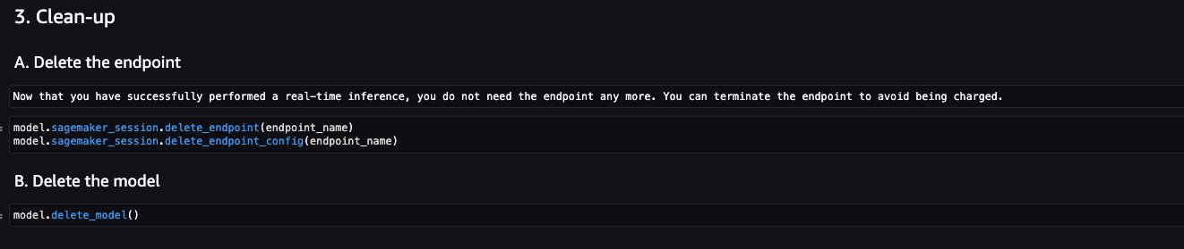
Clean up
After you have completed your work with SageMaker Canvas, choose Log out to close the session and avoid any further cost.

When you log out, your work such as datasets and models remains saved, and you can launch a SageMaker Canvas session again to continue the work later.
SageMaker Canvas creates an asynchronous SageMaker endpoint for generating the predictions. To delete the endpoint, endpoint configuration, and model created by SageMaker Canvas, refer to Delete Endpoints and Resources.
Conclusion
In this post, you learned how to use SageMaker Canvas to build an image classification model to predict defects in manufactured products, to compliment and improve the visual inspection quality process. You can use SageMaker Canvas with different image datasets from your manufacturing environment to build models for use cases like predictive maintenance, package inspection, worker safety, goods tracking, and more. SageMaker Canvas gives you the ability to use ML to generate predictions without needing to write any code, accelerating the evaluation and adoption of CV ML capabilities.
To get started and learn more about SageMaker Canvas, refer to the following resources:
- Amazon SageMaker Canvas Developer Guide
- Announcing Amazon SageMaker Canvas – a Visual, No Code Machine Learning Capability for Business Analysts
About the authors
 Brajendra Singh is solution architect in Amazon Web Services working with enterprise customers. He has strong developer background and is a keen enthusiast for data and machine learning solutions.
 Danny Smith is Principal, ML Strategist for Automotive and Manufacturing Industries, serving as a strategic advisor for customers. His career focus has been on helping key decision-makers leverage data, technology and mathematics to make better decisions, from the board room to the shop floor. Lately most of his conversations are on democratizing machine learning and generative AI.
 Davide Gallitelli is a Specialist Solutions Architect for AI/ML in the EMEA region. He is based in Brussels and works closely with customers throughout Benelux. He has been a developer since he was very young, starting to code at the age of 7. He started learning AI/ML at university, and has fallen in love with it since then.
 Gilles-Kuessan Satchivi is an AWS Enterprise Solutions Architect with a background in networking, infrastructure, security, and IT operations. He is passionate about helping customers build Well-Architected systems on AWS. Before joining AWS, he worked in ecommerce for 17 years. Outside of work, he likes to spend time with his family and cheer on his children’s soccer team.
 Aditya Pendyala is a Senior Solutions Architect at AWS based out of NYC. He has extensive experience in architecting cloud-based applications. He is currently working with large enterprises to help them craft highly scalable, flexible, and resilient cloud architectures, and guides them on all things cloud. He has a Master of Science degree in Computer Science from Shippensburg University and believes in the quote “When you cease to learn, you cease to grow.”
 Prabhakar Chandrasekaran is a Senior Technical Account Manager with AWS Enterprise Support. Prabhakar enjoys helping customers build cutting-edge AI/ML solutions on the cloud. He also works with enterprise customers providing proactive guidance and operational assistance, helping them improve the value of their solutions when using AWS. Prabhakar holds six AWS and six other professional certifications. With over 20 years of professional experience, Prabhakar was a data engineer and a program leader in the financial services space prior to joining AWS.

 Sean Morgan is a Senior ML Solutions Architect at AWS. He has experience in the semiconductor and academic research fields, and uses his experience to help customers reach their goals on AWS. In his free time, Sean is an active open-source contributor and maintainer, and is the special interest group lead for TensorFlow Addons.
 Lauren Mullennex is a Senior AI/ML Specialist Solutions Architect at AWS. She has a decade of experience in DevOps, infrastructure, and ML. She is also the author of a book on computer vision. Her other areas of focus include MLOps and generative AI.
 Philipp Schmid is a Technical Lead at Hugging Face with the mission to democratize good machine learning through open source and open science. Philipp is passionate about productionizing cutting-edge and generative AI machine learning models. He loves to share his knowledge on AI and NLP at various meetups such as Data Science on AWS, and on his technical
 Henrik Balle is a Sr. Solutions Architect at AWS supporting the US Public Sector. He works closely with customers on a range of topics from machine learning to security and governance at scale. In his spare time, he loves road biking, motorcycling, or you might find him working on yet another home improvement project.


 June Won is a product manager with SageMaker JumpStart. He focuses on making foundation models easily discoverable and usable to help customers build generative AI applications.
 Mani Khanuja is an Artificial Intelligence and Machine Learning Specialist SA at Amazon Web Services (AWS). She helps customers using machine learning to solve their business challenges using the AWS. She spends most of her time diving deep and teaching customers on AI/ML projects related to computer vision, natural language processing, forecasting, ML at the edge, and more. She is passionate about ML at edge, therefore, she has created her own lab with self-driving kit and prototype manufacturing production line, where she spends lot of her free time.
 Nitin Eusebius is a Sr. Enterprise Solutions Architect at AWS with experience in Software Engineering , Enterprise Architecture and AI/ML. He works with customers on helping them build well-architected applications on the AWS platform. He is passionate about solving technology challenges and helping customers with their cloud journey.