Four CVPR papers from Prime Video examine a broad set of topics related to efficient model training for understanding and synthesizing long-form cinematic content.Read More
Use proprietary foundation models from Amazon SageMaker JumpStart in Amazon SageMaker Studio
Amazon SageMaker JumpStart is a machine learning (ML) hub that can help you accelerate your ML journey. With SageMaker JumpStart, you can discover and deploy publicly available and proprietary foundation models to dedicated Amazon SageMaker instances for your generative AI applications. SageMaker JumpStart allows you to deploy foundation models from a network isolated environment, and doesn’t share customer training and inference data with model providers.
In this post, we walk through how to get started with proprietary models from model providers such as AI21, Cohere, and LightOn from Amazon SageMaker Studio. SageMaker Studio is a notebook environment where SageMaker enterprise data scientist customers evaluate and build models for their next generative AI applications.
Foundation models in SageMaker
Foundation models are large-scale ML models that contain billions of parameters and are pre-trained on terabytes of text and image data so you can perform a wide range of tasks, such as article summarization and text, image, or video generation. Because foundation models are pre-trained, they can help lower training and infrastructure costs and enable customization for your use case.
SageMaker JumpStart provides two types of foundation models:
- Proprietary models – These models are from providers such as AI21 with Jurassic-2 models, Cohere with Cohere Command, and LightOn with Mini trained on proprietary algorithms and data. You can’t view model artifacts such as weight and scripts, but you can still deploy to SageMaker instances for inferencing.
- Publicly available models – These are from popular model hubs such as Hugging Face with Stable Diffusion, Falcon, and FLAN trained on publicly available algorithms and data. For these models, users have access to model artifacts and are able to fine-tune with their own data prior to deployment for inferencing.
Discover models
You can access the foundation models through SageMaker JumpStart in the SageMaker Studio UI and the SageMaker Python SDK. In this section, we go over how to discover the models in the SageMaker Studio UI.
SageMaker Studio is a web-based integrated development environment (IDE) for ML that lets you build, train, debug, deploy, and monitor your ML models. For more details on how to get started and set up SageMaker Studio, refer to Amazon SageMaker Studio.
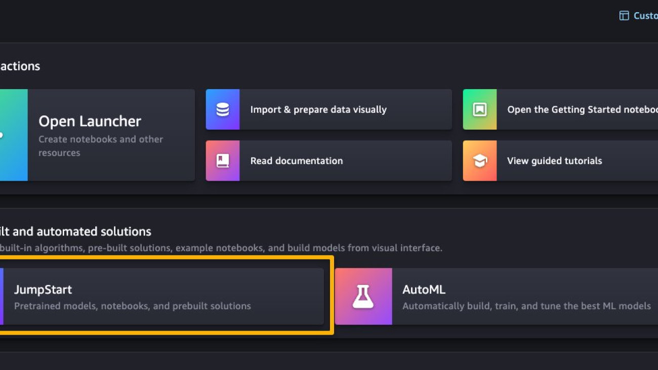
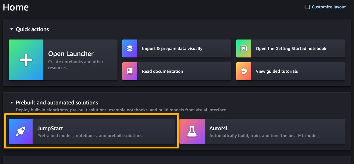
Once you’re on the SageMaker Studio UI, you can access SageMaker JumpStart, which contains pre-trained models, notebooks, and prebuilt solutions, under Prebuilt and automated solutions.
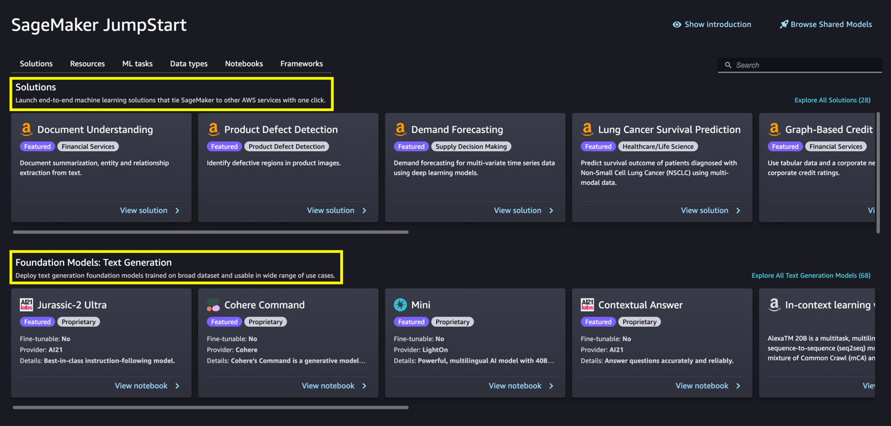
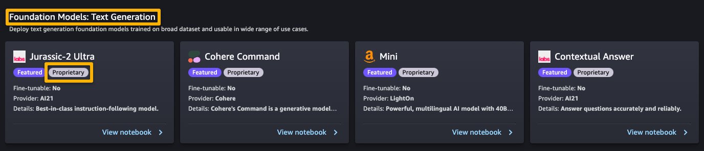
From the SageMaker JumpStart landing page, you can browse for solutions, models, notebooks, and other resources. The following screenshot shows an example of the landing page with solutions and foundation models listed.
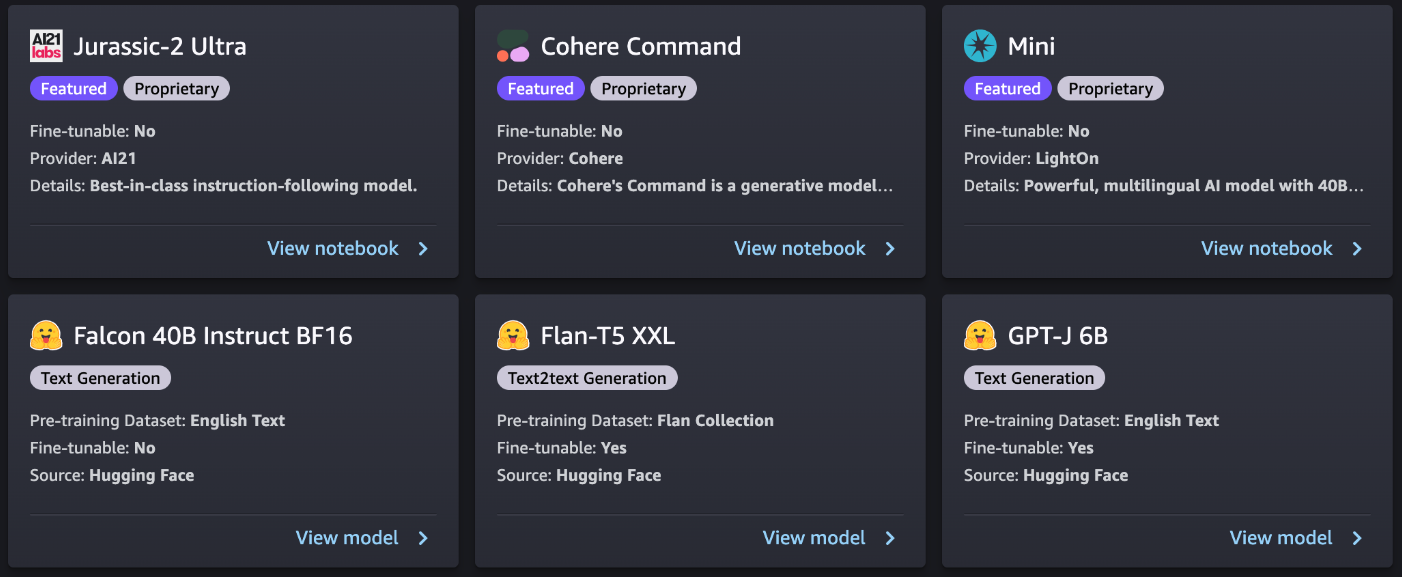
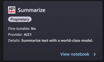
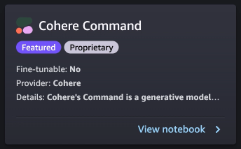
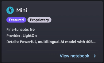
Each model has a model card, as shown in the following screenshot, which contains the model name, if it is fine-tunable or not, the provider name, and a short description about the model. You can also open the model card to learn more about the model and start training or deploying.
Subscribe in AWS Marketplace
Proprietary models in SageMaker JumpStart are published by model providers such as AI21, Cohere, and LightOn. You can identify proprietary models by the “Proprietary” tag on model cards, as shown in the following screenshot.
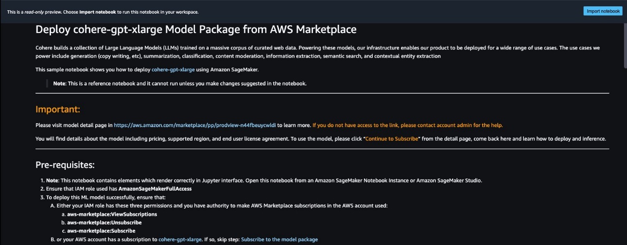
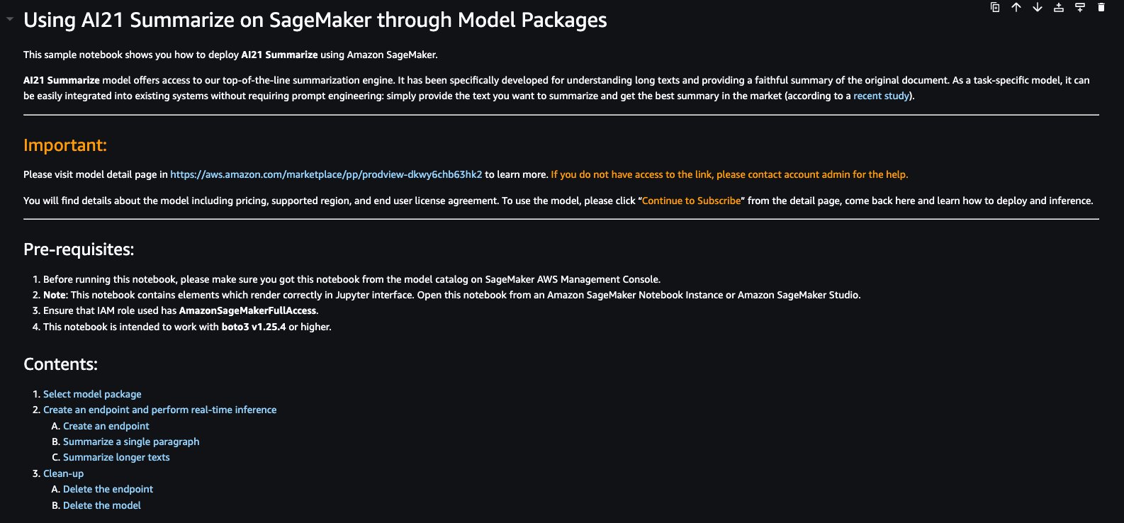
You can choose View notebook on the model card to open the notebook in read-only mode, as shown in the following screenshot. You can read the notebook for important information regarding prerequisites and other usage instructions.
After importing the notebook, you need to select the appropriate notebook environment (image, kernel, instance type, and so on) before running codes. You should also follow the subscription and usage instructions per the selected notebook.
Before using a proprietary model, you need to first subscribe to the model from AWS Marketplace:
- Open the model listing page in AWS Marketplace.
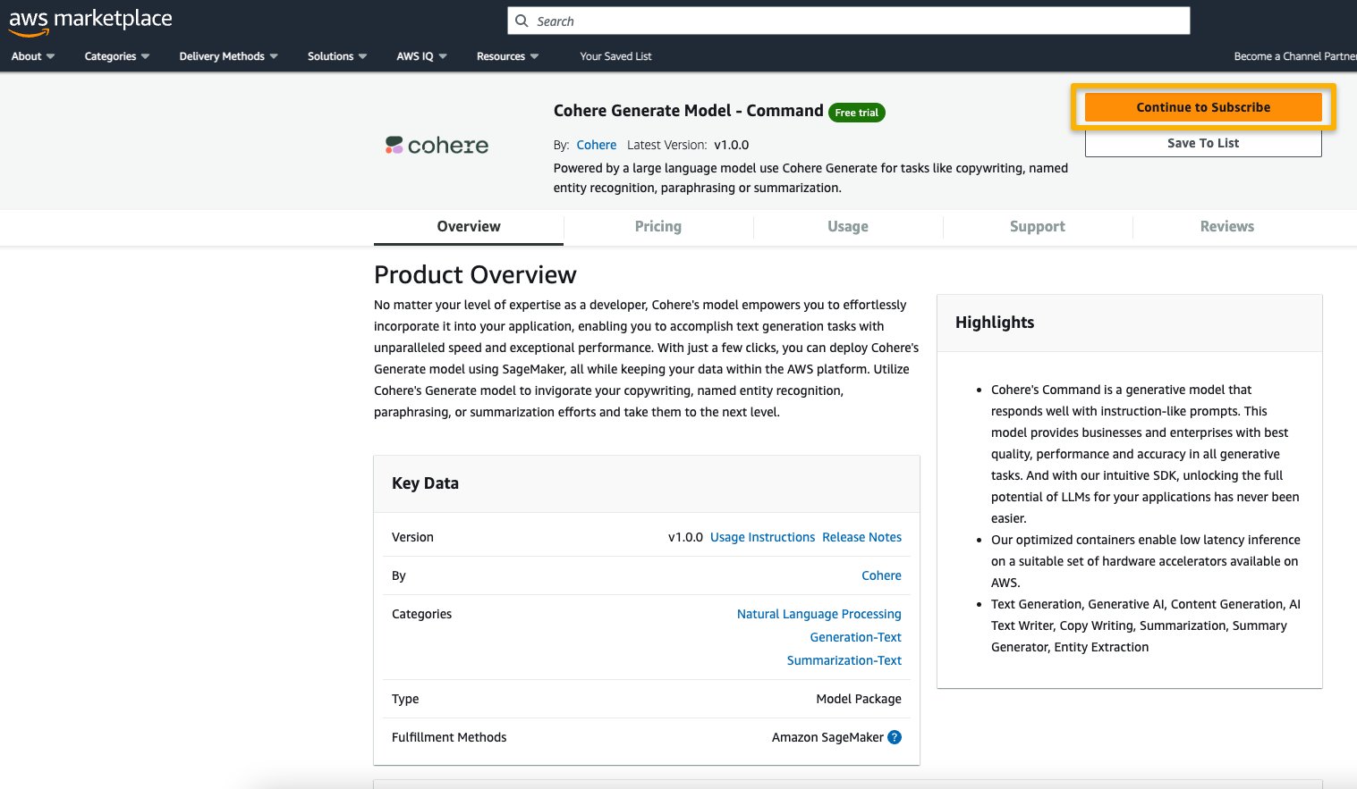
The URL is provided in the Important section of the notebook, or you can access it from the SageMaker JumpStart service page. The listing page shows the overview, pricing, usage, and support information about the model.
- On the AWS Marketplace listing, choose Continue to subscribe.
If you don’t have the necessary permissions to view or subscribe to the model, reach out to your IT admin or procurement point of contact to subscribe to the model for you. Many enterprises may limit AWS Marketplace permissions to control the actions that someone with those permissions can take in the AWS Marketplace Management Portal.
- On the Subscribe to this software page, review the details and choose Accept offer if you and your organization agree with the EULA, pricing, and support terms.
If you have any questions or a request for volume discount, reach out to the model provider directly via the support email provided on the detail page or reach out to your AWS account team.
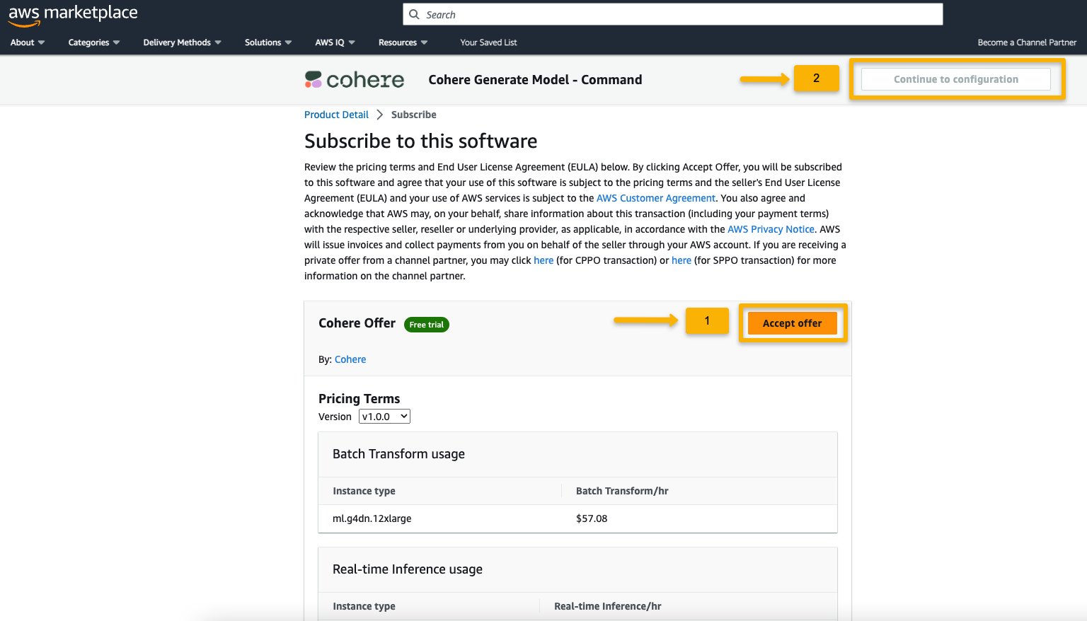
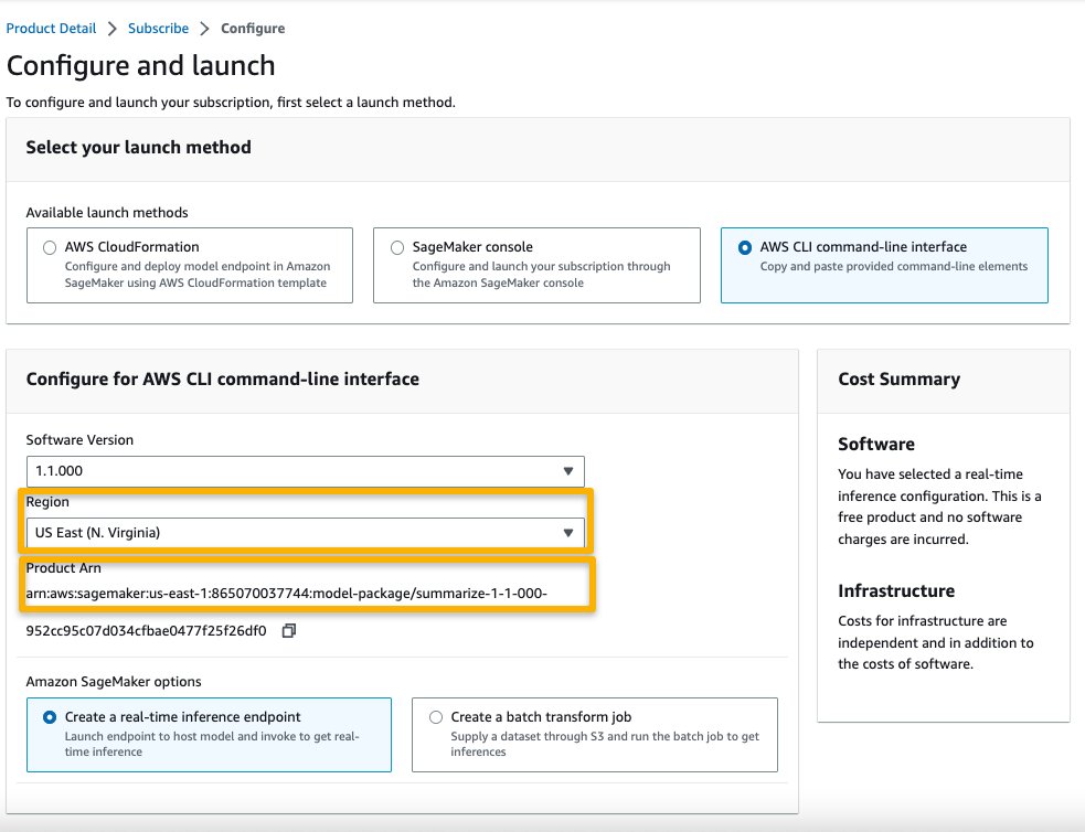
- Choose Continue to configuration and choose a Region.
You will see a product ARN displayed. This is the model package ARN that you need to specify while creating a deployable model using Boto3.
- Copy the ARN corresponding to your Region and specify the same in the notebook’s cell instruction.
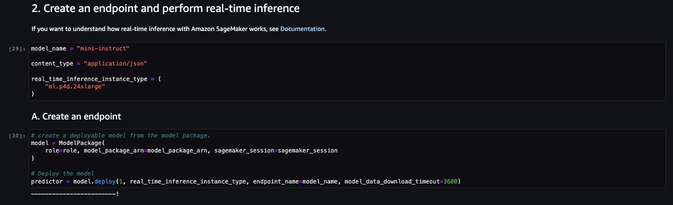
Sample inferencing with sample prompts
Let’s look at some of the sample foundation models from A21 Labs, Cohere, and LightOn that are discoverable from SageMaker JumpStart in SageMaker Studio. All of them have same the instructions to subscribe from AWS Marketplace and import and configure the notebook.
AI21 Summarize
The Summarize model by A121 Labs condenses lengthy texts into short, easy-to-read bites that remain factually consistent with the source. The model is trained to generate summaries that capture key ideas based on a body of text. It doesn’t require any prompting. You simply input the text that needs to be summarized. Your source text can contain up to 50,000 characters, translating to roughly 10,000 words, or an impressive 40 pages.
The sample notebook for AI21 Summarize model provides important prerequisites that needs to be followed. For example the model is subscribed from AWS Marketplace , have appropriate IAM roles permissions, and required boto3 version etc. It walks you through how to select the model package, create endpoints for real-time inference, and then clean up.
The selected model package contains the mapping of ARNs to Regions. This is the information you captured after choosing Continue to configuration on the AWS Marketplace subscription page (in the section Evaluate and subscribe in Marketplace) and then selecting a Region for which you will see the corresponding product ARN.
The notebook may already have ARN prepopulated.

You then import some libraries required to run this notebook and install wikipedia, which is a Python library that makes it easy to access and parse data from Wikipedia. The notebook uses this later to showcase how to summarize a long text from Wikipedia.
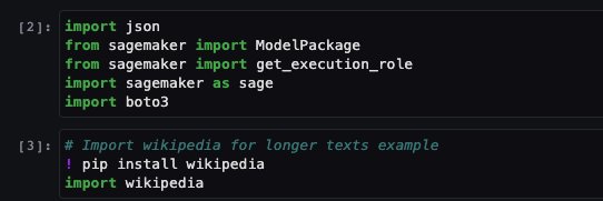
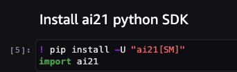
The notebook also proceeds to install the ai21 Python SDK, which is a wrapper around SageMaker APIs such as deploy and invoke endpoint.
The next few cells of the notebook walk through the following steps:
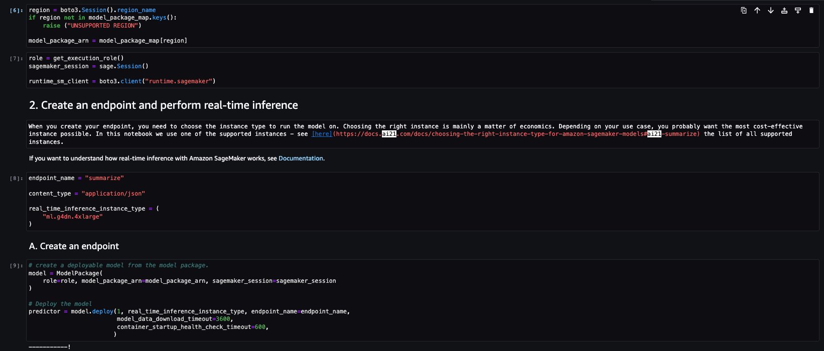
- Select the Region and fetch the model package ARN from model package map
- Create your inference endpoint by selecting an instance type (depending on your use case and supported instance for the model; see Task-specific models for more details) to run the model on
- Create a deployable model from the model package
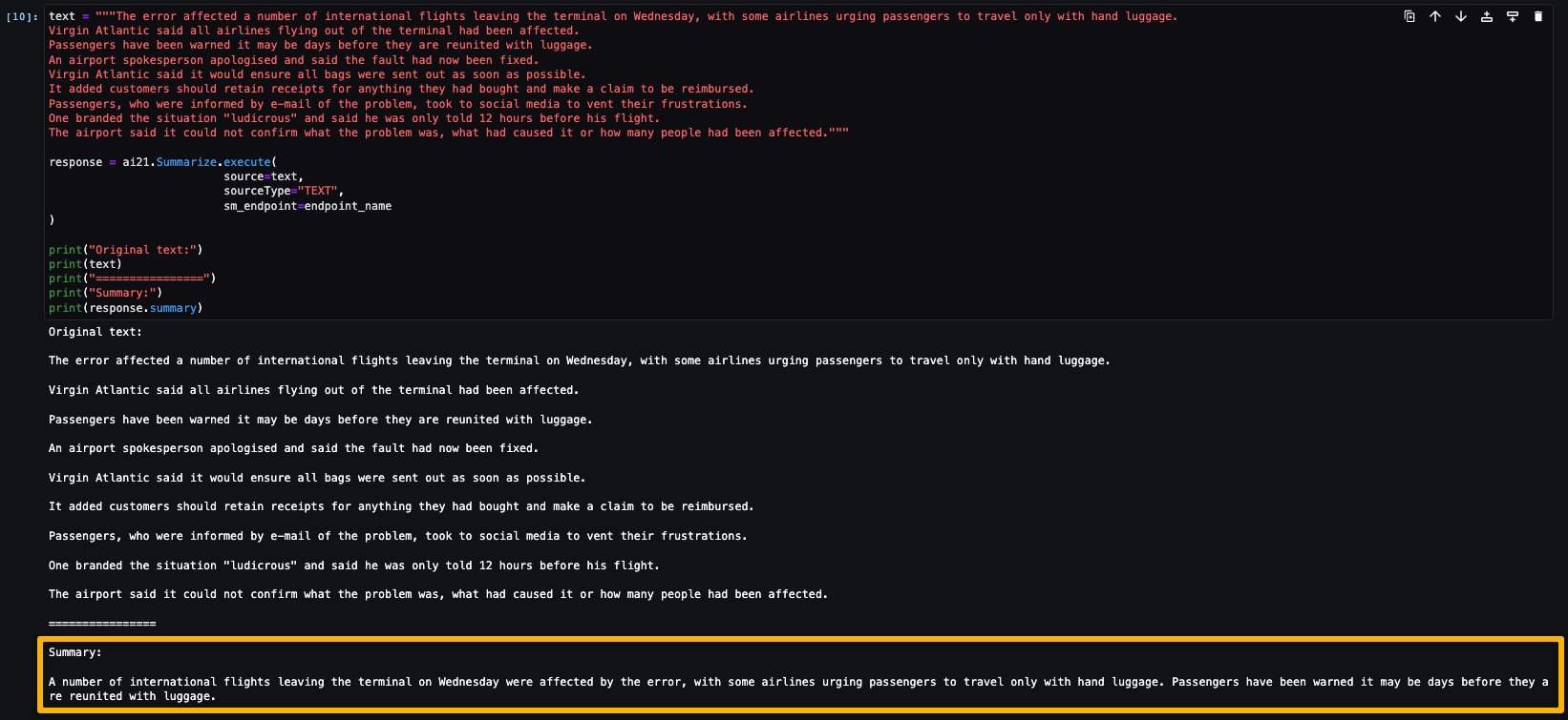
Let’s run the inference to generate a summary of a single paragraph taken from a news article. As you can see in the output, the summarized text is presented as an output by the model.
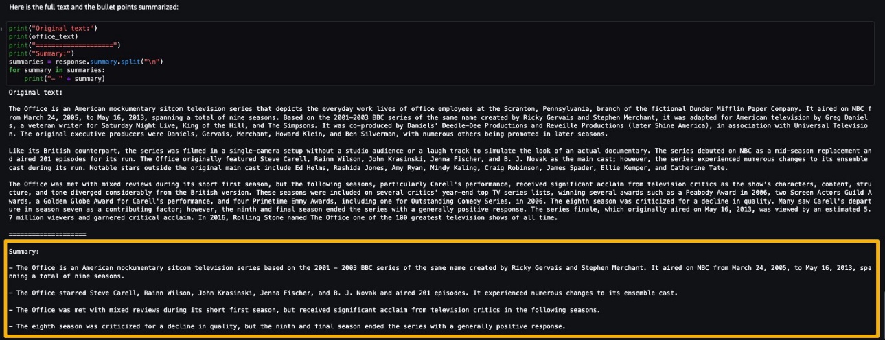
AI21 Summarize can handle inputs up to 50,000 characters. This translates into roughly 10,000 words, or 40 pages. As a demonstration of the model’s behavior, we load a page from Wikipedia.

Now that you have performed a real-time inference for testing, you may not need the endpoint anymore. You can delete the endpoint to avoid being charged.
Cohere Command
Cohere Command is a generative model that responds well with instruction-like prompts. This model provides businesses and enterprises with best quality, performance, and accuracy in all generative tasks. You can use Cohere’s Command model to invigorate your copywriting, named entity recognition, paraphrasing, or summarization efforts and take them to the next level.
The sample notebook for Cohere Command model provides important prerequisites that needs to be followed. For example the model is subscribed from AWS Marketplace, have appropriate IAM roles permissions, and required boto3 version etc. It walks you through how to select the model package, create endpoints for real-time inference, and then clean up.
Some of the tasks are similar to those covered in the previous notebook example, like installing Boto3, installing cohere-sagemaker (the package provides functionality developed to simplify interfacing with the Cohere model), and getting the session and Region.
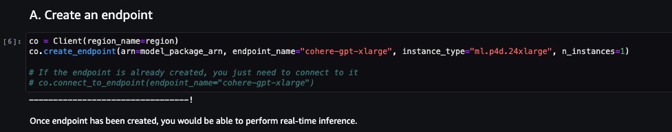
Let’s explore creating the endpoint. You provide the model package ARN, endpoint name, instance type to be used, and number of instances. Once created, the endpoint appears in your endpoint section of SageMaker.
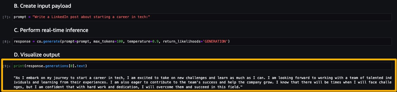
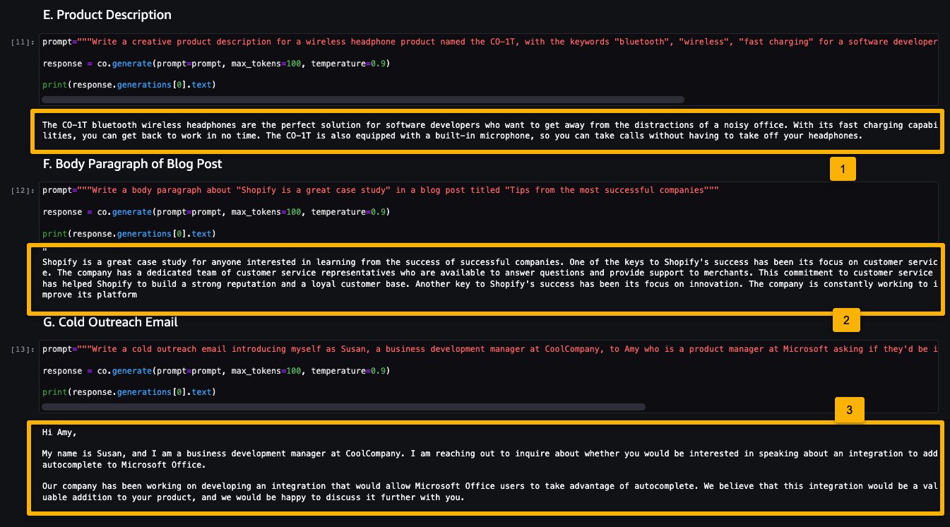
Now let’s run the inference to see some of the outputs from the Command model.
The following screenshot shows a sample example of generating a job post and its output. As you can see, the model generated a post from the given prompt.
Now let’s look at the following examples:
- Generate a product description
- Generate a body paragraph of a blog post
- Generate an outreach email
As you can see, the Cohere Command model generated text for various generative tasks.
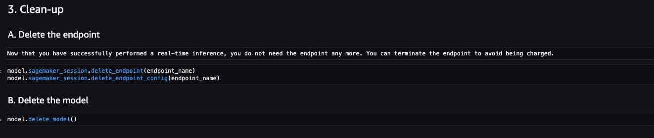
Now that you have performed real-time inference for testing, you may not need the endpoint anymore. You can delete the endpoint to avoid being charged.
LightOn Mini-instruct
Mini-instruct, an AI model with 40 billion billion parameters created by LightOn, is a powerful multilingual AI system that has been trained using high-quality data from numerous sources. It is built to understand natural language and react to commands that are specific to your needs. It performs admirably in consumer products like voice assistants, chatbots, and smart appliances. It also has a wide range of business applications, including agent assistance and natural language production for automated customer care.
The sample notebook for LightOn Mini-instruct model provides important prerequisites that needs to be followed. For example the model is subscribed from AWS Marketplace, have appropriate IAM roles permissions, and required boto3 version etc. It walks you through how to select the model package, create endpoints for real-time inference, and then clean up.
Some of the tasks are similar to those covered in the previous notebook example, like installing Boto3 and getting the session Region.
Let’s look at creating the endpoint. First, provide the model package ARN, endpoint name, instance type to be used, and number of instances. Once created, the endpoint appears in your endpoint section of SageMaker.
Now let’s try inferencing the model by asking it to generate a list of ideas for articles for a topic, in this case watercolor.
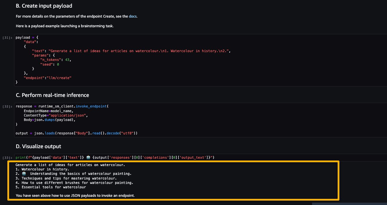
As you can see, the LightOn Mini-instruct model was able to provide generated text based on the given prompt.
Clean up
After you have tested the models and created endpoints above for the example proprietary Foundation Models, make sure you delete the SageMaker inference endpoints and delete the models to avoid incurring charges.
Conclusion
In this post, we showed you how to get started with proprietary models from model providers such as AI21, Cohere, and LightOn in SageMaker Studio. Customers can discover and use proprietary Foundation Models in SageMaker JumpStart from Studio, the SageMaker SDK, and the SageMaker Console. With this, they have access to large-scale ML models that contain billions of parameters and are pretrained on terabytes of text and image data so customers can perform a wide range of tasks such as article summarization and text, image, or video generation. Because foundation models are pretrained, they can also help lower training and infrastructure costs and enable customization for your use case.
Resources
- SageMaker JumpStart documentation
- SageMaker JumpStart Foundation Models documentation
- SageMaker JumpStart product detail page
- SageMaker JumpStart model catalog
About the authors
 June Won is a product manager with SageMaker JumpStart. He focuses on making foundation models easily discoverable and usable to help customers build generative AI applications.
 Mani Khanuja is an Artificial Intelligence and Machine Learning Specialist SA at Amazon Web Services (AWS). She helps customers using machine learning to solve their business challenges using the AWS. She spends most of her time diving deep and teaching customers on AI/ML projects related to computer vision, natural language processing, forecasting, ML at the edge, and more. She is passionate about ML at edge, therefore, she has created her own lab with self-driving kit and prototype manufacturing production line, where she spends lot of her free time.
 Nitin Eusebius is a Sr. Enterprise Solutions Architect at AWS with experience in Software Engineering , Enterprise Architecture and AI/ML. He works with customers on helping them build well-architected applications on the AWS platform. He is passionate about solving technology challenges and helping customers with their cloud journey.
How Earth.com and Provectus implemented their MLOps Infrastructure with Amazon SageMaker
This blog post is co-written with Marat Adayev and Dmitrii Evstiukhin from Provectus.
When machine learning (ML) models are deployed into production and employed to drive business decisions, the challenge often lies in the operation and management of multiple models. Machine Learning Operations (MLOps) provides the technical solution to this issue, assisting organizations in managing, monitoring, deploying, and governing their models on a centralized platform.
At-scale, real-time image recognition is a complex technical problem that also requires the implementation of MLOps. By enabling effective management of the ML lifecycle, MLOps can help account for various alterations in data, models, and concepts that the development of real-time image recognition applications is associated with.
One such application is EarthSnap, an AI-powered image recognition application that enables users to identify all types of plants and animals, using the camera on their smartphone. EarthSnap was developed by Earth.com, a leading online platform for enthusiasts who are passionate about the environment, nature, and science.
Earth.com’s leadership team recognized the vast potential of EarthSnap and set out to create an application that utilizes the latest deep learning (DL) architectures for computer vision (CV). However, they faced challenges in managing and scaling their ML system, which consisted of various siloed ML and infrastructure components that had to be maintained manually. They needed a cloud platform and a strategic partner with proven expertise in delivering production-ready AI/ML solutions, to quickly bring EarthSnap to the market. That is where Provectus, an AWS Premier Consulting Partner with competencies in Machine Learning, Data & Analytics, and DevOps, stepped in.
This post explains how Provectus and Earth.com were able to enhance the AI-powered image recognition capabilities of EarthSnap, reduce engineering heavy lifting, and minimize administrative costs by implementing end-to-end ML pipelines, delivered as part of a managed MLOps platform and managed AI services.
Challenges faced in the initial approach
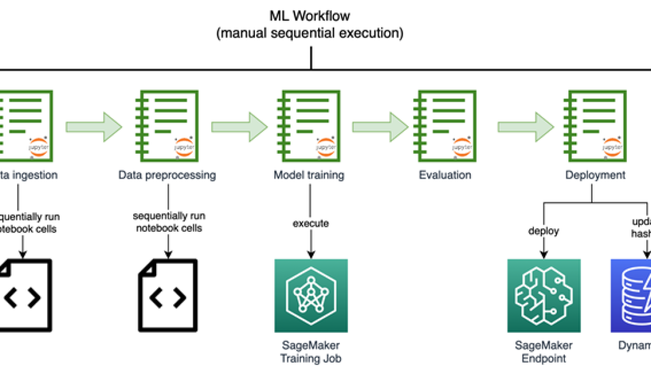
The executive team at Earth.com was eager to accelerate the launch of EarthSnap. They swiftly began to work on AI/ML capabilities by building image recognition models using Amazon SageMaker. The following diagram shows the initial image recognition ML workflow, run manually and sequentially.
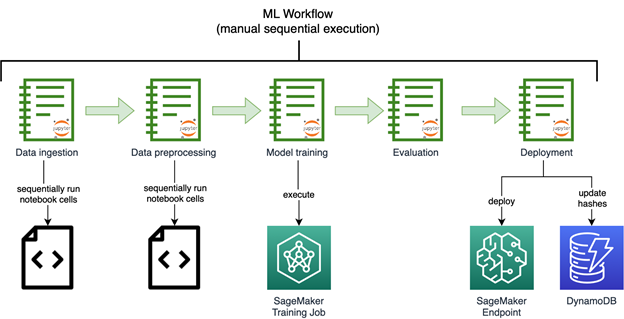
The models developed by Earth.com lived across various notebooks. They required the manual sequential execution run of a series of complex notebooks to process the data and retrain the model. Endpoints had to be deployed manually as well.
Earth.com didn’t have an in-house ML engineering team, which made it hard to add new datasets featuring new species, release and improve new models, and scale their disjointed ML system.
The ML components for data ingestion, preprocessing, and model training were available as disjointed Python scripts and notebooks, which required a lot of manual heavy lifting on the part of engineers.
The initial solution also required the support of a technical third party, to release new models swiftly and efficiently.
First iteration of the solution
Provectus served as a valuable collaborator for Earth.com, playing a crucial role in augmenting the AI-driven image recognition features of EarthSnap. The application’s workflows were automated by implementing end-to-end ML pipelines, which were delivered as part of Provectus’s managed MLOps platform and supported through managed AI services.
A series of project discovery sessions were initiated by Provectus to examine EarthSnap’s existing codebase and inventory the notebook scripts, with the goal of reproducing the existing model results. After the model results had been restored, the scattered components of the ML workflow were merged into an automated ML pipeline using Amazon SageMaker Pipelines, a purpose-built CI/CD service for ML.
The final pipeline includes the following components:
- Data QA & versioning – This step run as a SageMaker Processing job, ingests the source data from Amazon Simple Storage Service (Amazon S3) and prepares the metadata for the next step, containing only valid images (URI and label) that are filtered according to internal rules. It also persists a manifest file to Amazon S3, including all necessary information to recreate that dataset version.
- Data preprocessing – This includes multiple steps wrapped as SageMaker processing jobs, and run sequentially. The steps preprocess the images, convert them to RecordIO format, split the images into datasets (full, train, test and validation), and prepare the images to be consumed by SageMaker training jobs.
- Hyperparameter tuning – A SageMaker hyperparameter tuning job takes as input a subset of the training and validation set and runs a series of small training jobs under the hood to determine the best parameters for the full training job.
- Full training – A step SageMaker training job launches the training job on the entire data, given the best parameters from the hyperparameter tuning step.
- Model evaluation – A step SageMaker processing job is run after the final model has been trained. This step produces an expanded report containing the model’s metrics.
- Model creation – The SageMaker ModelCreate step wraps the model into the SageMaker model package and pushes it to the SageMaker model registry.
All steps are run in an automated manner after the pipeline has been run. The pipeline can be run via any of following methods:
- Automatically using AWS CodeBuild, after the new changes are pushed to a primary branch and a new version of the pipeline is upserted (CI)
- Automatically using Amazon API Gateway, which can be triggered with a certain API call
- Manually in Amazon SageMaker Studio
After the pipeline run (launched using one of preceding methods), a trained model is produced that is ready to be deployed as a SageMaker endpoint. This means that the model must first be approved by the PM or engineer in the model registry, then the model is automatically rolled out to the stage environment using Amazon EventBridge and tested internally. After the model is confirmed to be working as expected, it’s deployed to the production environment (CD).
The Provectus solution for EarthSnap can be summarized in the following steps:
- Start with fully automated, end-to-end ML pipelines to make it easier for Earth.com to release new models
- Build on top of the pipelines to deliver a robust ML infrastructure for the MLOps platform, featuring all components for streamlining AI/ML
- Support the solution by providing managed AI services (including ML infrastructure provisioning, maintenance, and cost monitoring and optimization)
- Bring EarthSnap to its desired state (mobile application and backend) through a series of engagements, including AI/ML work, data and database operations, and DevOps
After the foundational infrastructure and processes were established, the model was trained and retrained on a larger dataset. At this point, however, the team encountered an additional issue when attempting to expand the model with even larger datasets. We needed to find a way to restructure the solution architecture, making it more sophisticated and capable of scaling effectively. The following diagram shows the EarthSnap AI/ML architecture.
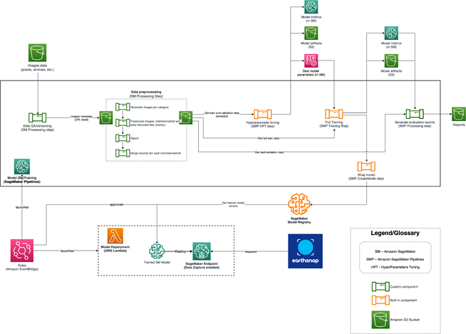
The AI/ML architecture for EarthSnap is designed around a series of AWS services:
- Sagemaker Pipeline runs using one of the methods mentioned above (CodeBuild, API, manual) that trains the model and produces artifacts and metrics. As a result, the new version of the model is pushed to the Sagemaker Model registry
- Then the model is reviewed by an internal team (PM/engineer) in model registry and approved/rejected based on metrics provided
- Once the model is approved, the model version is automatically deployed to the stage environment using the Amazon EventBridge that tracks the model status change
- The model is deployed to the production environment if the model passes all tests in the stage environment
Final solution
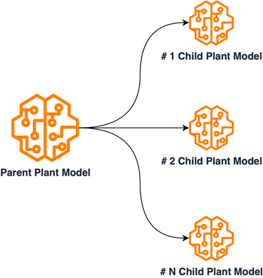
To accommodate all necessary sets of labels, the solution for EarthSnap’s model required substantial modifications, because incorporating all species within a single model proved to be both costly and inefficient. The plant category was selected first for implementation.
A thorough examination of plant data was conducted, to organize it into subsets based on shared internal characteristics. The solution for the plant model was redesigned by implementing a multi-model parent/child architecture. This was achieved by training child models on grouped subsets of plant data and training the parent model on a set of data samples from each subcategory. The Child models were employed for accurate classification within the internally grouped species, while the parent model was utilized to categorize input plant images into subgroups. This design necessitated distinct training processes for each model, leading to the creation of separate ML pipelines. With this new design, along with the previously established ML/MLOps foundation, the EarthSnap application was able to encompass all essential plant species, resulting in improved efficiency concerning model maintenance and retraining. The following diagram illustrates the logical scheme of parent/child model relations.
Upon completing the redesign, the ultimate challenge was to guarantee that the AI solution powering EarthSnap could manage the substantial load generated by a broad user base. Fortunately, the managed AI onboarding process encompasses all essential automation, monitoring, and procedures for transitioning the solution into a production-ready state, eliminating the need for any further capital investment.
Results
Despite the pressing requirement to develop and implement the AI-driven image recognition features of EarthSnap within a few months, Provectus managed to meet all project requirements within the designated time frame. In just 3 months, Provectus modernized and productionized the ML solution for EarthSnap, ensuring that their mobile application was ready for public release.
The modernized infrastructure for ML and MLOps allowed Earth.com to reduce engineering heavy lifting and minimize the administrative costs associated with maintenance and support of EarthSnap. By streamlining processes and implementing best practices for CI/CD and DevOps, Provectus ensured that EarthSnap could achieve better performance while improving its adaptability, resilience, and security. With a focus on innovation and efficiency, we enabled EarthSnap to function flawlessly, while providing a seamless and user-friendly experience for all users.
As part of its managed AI services, Provectus was able to reduce the infrastructure management overhead, establish well-defined SLAs and processes, ensure 24/7 coverage and support, and increase overall infrastructure stability, including production workloads and critical releases. We initiated a series of enhancements to deliver managed MLOps platform and augment ML engineering. Specifically, it now takes Earth.com minutes, instead of several days, to release new ML models for their AI-powered image recognition application.
With assistance from Provectus, Earth.com was able to release its EarthSnap application at the Apple Store and Playstore ahead of schedule. The early release signified the importance of Provectus’ comprehensive work for the client.
”I’m incredibly excited to work with Provectus. Words can’t describe how great I feel about handing over control of the technical side of business to Provectus. It is a huge relief knowing that I don’t have to worry about anything other than developing the business side.”
– Eric Ralls, Founder and CEO of EarthSnap.
The next steps of our cooperation will include: adding advanced monitoring components to pipelines, enhancing model retraining, and introducing a human-in-the-loop step.
Conclusion
The Provectus team hopes that Earth.com will continue to modernize EarthSnap with us. We look forward to powering the company’s future expansion, further popularizing natural phenomena, and doing our part to protect our planet.
To learn more about the Provectus ML infrastructure and MLOps, visit Machine Learning Infrastructure and watch the webinar for more practical advice. You can also learn more about Provectus managed AI services at the Managed AI Services.
If you’re interested in building a robust infrastructure for ML and MLOps in your organization, apply for the ML Acceleration Program to get started.
Provectus helps companies in healthcare and life sciences, retail and CPG, media and entertainment, and manufacturing, achieve their objectives through AI.
Provectus is an AWS Machine Learning Competency Partner and AI-first transformation consultancy and solutions provider helping design, architect, migrate, or build cloud-native applications on AWS.
Contact Provectus | Partner Overview
About the Authors
Marat Adayev is an ML Solutions Architect at Provectus
Dmitrii Evstiukhin is the Director of Managed Services at Provectus
James Burdon is a Senior Startups Solutions Architect at AWS
Amazon and Max Planck Society announce sustainability awards
Two Max Planck Society researchers receive funding for projects to develop new ways to advance a more circular economy.Read More
Define customized permissions in minutes with Amazon SageMaker Role Manager via the AWS CDK
Machine learning (ML) administrators play a critical role in maintaining the security and integrity of ML workloads. Their primary focus is to ensure that users operate with the utmost security, adhering to the principle of least privilege. However, accommodating the diverse needs of different user personas and creating appropriate permission policies can sometimes impede agility. To address this challenge, AWS introduced Amazon SageMaker Role Manager in December 2022. SageMaker Role Manager is a powerful tool can you can use to swiftly develop persona-based roles, which can be easily customized to meet specific requirements.
With SageMaker Role Manager, administrators can efficiently define persona-based roles tailored to distinct user groups. This approach ensures that individuals have access only to the resources and actions essential for their tasks, reducing the risk of unauthorized actions or breaches. SageMaker Role Manager also allows for fine-grained customization. ML administrators can tailor the roles to meet specific requirements by modifying the permissions associated with each persona. This flexibility ensures that the permissions align precisely with the tasks and responsibilities of individual users, providing a robust security framework while accommodating unique use cases.
SageMaker Role Manager is currently available on the Amazon SageMaker console of all commercial Regions. Today, we are launching the ability to define customized permissions in minutes with SageMaker Role Manager via the AWS Cloud Development Kit (AWS CDK). This addresses a critical obstacle to wider adoption because ML administrators can now automate their tasks programmatically. With the power of the AWS CDK, ML administrators can streamline workflows, reduce manual efforts, and ensure consistency in managing permissions for their ML infrastructure.
Solution overview
With the release of the SageMaker Role Manager CDK, we are launching two new infrastructure as code (IaC) capabilities:
- Create fine-grained permissions for ML personas
- Create fine-grained permissions for automated jobs through Amazon SageMaker Pipelines, AWS Lambda, and other AWS services
You can create fine-grained AWS Identity and Access Management (IAM) roles for ML personas such as data scientist, ML engineer, or data engineer. SageMaker Role Manager offers predefined personas and ML activities combined to streamline your permission generation process, allowing your ML practitioners to perform their responsibilities with the least privilege permissions. For secure access to your ML resources, SageMaker Role Manager allows you to specify networking and encryption permissions for Amazon Virtual Private Cloud (Amazon VPC) resources and AWS Key Management Service (AWS KMS) encryption keys. Furthermore, you can customize permissions by attaching your own customer managed policies.
The SageMaker Role Manager CDK lets you define custom permissions for SageMaker users in minutes. It comes with a set of predefined policy templates for different personas and ML activities. Personas represent the different types of users that need permissions to perform ML activities in SageMaker, such as data scientists or MLOps engineers. ML activities are a set of permissions to accomplish a common ML task, such as running Amazon SageMaker Studio applications or managing experiments, models, or pipelines. After you have selected the persona type and the set of ML activities, the SageMaker Role Manager CDK automatically creates the required IAM role and policies that you can assign to SageMaker users. Similarly, you can also create IAM roles with fine-grained permissions for automated jobs such as running SageMaker Pipelines.
Prerequisites
To start using the SageMaker Role Manager CDK, you need to complete the following prerequisite steps:
- Set up a role for your ML administrator to create and manage personas, as well as the IAM permissions for those users. For a sample admin policy, refer to the prerequisite section in Define customized permissions in minutes with Amazon SageMaker Role Manager blog post.
- Create a compute-only persona role (if you don’t have any) for passing to jobs and endpoints. For instructions to set up that role, refer to Using the role manager.
- Set up your AWS CDK development environment. For instructions, refer to Getting started with the AWS CDK.
Install and run the SageMaker Role Manager CDK
Complete the following steps to set up the SageMaker Role Manager CDK:
- Create your AWS CDK app and give it a name; for example,
RoleManager. - Navigate to the
RoleManagerfolder and run the following command to create a blank typescript AWS CDK project: - Open
package.jsonand add the highlighted package as shown in the following code: - Run the following command to install the new
cdk-aws-sagemaker-role-managerpackage: - Navigate to the lib folder and replace
role_manager_stack.tswith the following code: - Replace
passRoleId,passRoleName,newRoleId,newRoleName, andnewRoleDescriptionbased on your requirements for role creation. - Navigate back to your AWS CDK app home folder and run the following command to verify the generated AWS CloudFormation template:
- Finally, run the following command to run the CloudFormation stack in your AWS account:
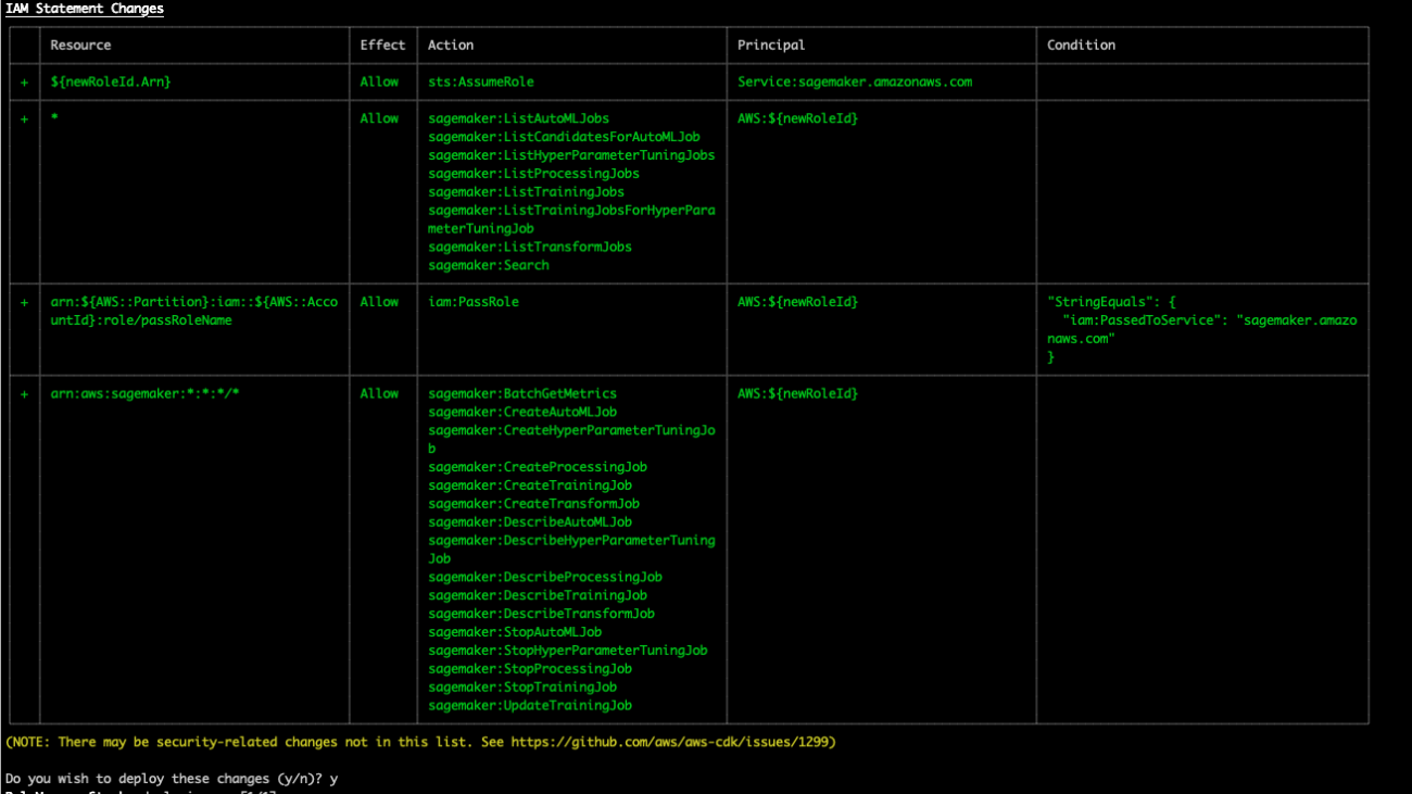
You should see an AWS CDK deployment output similar to the one in the following screenshot.

More SageMaker Role Manager CDK examples are available in the following GitHub repo.
ML persona and activity CDK reference
Administrators can define ML activities using one of the ML activity static functions of the ML activity class. For a list of the latest versions, refer to ML activity reference.
The ML persona class supports the following methods:
- customizeVPC(subnets, securityGroups) – Customizes the VPC of all activities that support VPC customization of personas.
- customizeKMS(dataKeys, volumeKeys) – Customizes KMS keys of all activities that support KMS key customization of personas.
- createRole(scope, id, roleNameSuffix, roleDescription) – Creates a role with the persona’s activities’ permissions similar to the UI in the scope with ID, with the name
SageMaker-${roleNameSuffix}and optionally with the passed role description. - grantPermissionsTo(identity) – Grants the persona’s activities’ permissions to the identity. The passed identity can be a role or an AWS resource associated with a role (for example, a Lambda function with the role of the Lambda function describing which resources the Lambda function can access).
- grantPermissionsTo() – Updates the role of the passed identity to have the permissions specified in the ML activity.
The ML activity class supports the same set of functions as ML personas; however, the difference is an ML activity is constrained to a single activity when using this interface to create IAM roles.
Conclusion
SageMaker Role Manager enables you to create customized roles based on personas, pre-built ML activities, and custom policies, significantly reducing the time required. Now, with this latest AWS CDK support, the ability to define roles is further expanded to support infrastructure as code. This empowers ML practitioners to work programmatically in SageMaker, enhancing efficiency and enabling seamless integration into their workflows.
We would like to hear from you on how this new feature is helping you. Try out the new AWS CDK support for SageMaker Role Manager and send us your feedback!
To learn more about how to use SageMaker Role Manager, refer to the SageMaker Role Manager Developer Guide.
About The Authors
 Akash Bhatia is a Principal Solution Architect with experience spanning multiple industries, including Manufacturing, Automotive, Retail ,and Space and Technology. Currently working in Amazon Web Services Enterprise Segments, Akash works closely with a diverse range of clients, including Fortune 100 companies and start-ups, to facilitate their cloud migration journey. In addition to his technical expertise, Akash has led product and program management, having successfully overseen numerous large-scale initiatives throughout his career.
 Ram Vittal is a Principal ML Solutions Architect at AWS. He has over 20 years of experience architecting and building distributed, hybrid, and cloud applications. He is passionate about building secure and scalable AI/ML and big data solutions to help enterprise customers with their cloud adoption and optimization journey to improve their business outcomes. In his spare time, he enjoys riding motorcycle, playing tennis, and photography.
 Ozan Eken is a Senior Product Manager at Amazon Web Services. He has over 15 years of experience in consulting and product management. He is passionate about building governance products, and Admin capabilities in Machine Learning for enterprise customers. Outside of work, he likes exploring different outdoor activities and watching soccer.
The science behind the improved Fire TV voice search
How phonetically blended results (PBR) help ensure customers find the content they were actually asking for.Read More
Accelerate time to business insights with the Amazon SageMaker Data Wrangler direct connection to Snowflake
Amazon SageMaker Data Wrangler is a single visual interface that reduces the time required to prepare data and perform feature engineering from weeks to minutes with the ability to select and clean data, create features, and automate data preparation in machine learning (ML) workflows without writing any code.
SageMaker Data Wrangler supports Snowflake, a popular data source for users who want to perform ML. We launch the Snowflake direct connection from the SageMaker Data Wrangler in order to improve the customer experience. Before the launch of this feature, administrators were required to set up the initial storage integration to connect with Snowflake to create features for ML in Data Wrangler. This includes provisioning Amazon Simple Storage Service (Amazon S3) buckets, AWS Identity and Access Management (IAM) access permissions, Snowflake storage integration for individual users, and an ongoing mechanism to manage or clean up data copies in Amazon S3. This process is not scalable for customers with strict data access control and a large number of users.
In this post, we show how Snowflake’s direct connection in SageMaker Data Wrangler simplifies the administrator’s experience and data scientist’s ML journey from data to business insights.
Solution overview
In this solution, we use SageMaker Data Wrangler to speed up data preparation for ML and Amazon SageMaker Autopilot to automatically build, train, and fine-tune the ML models based on your data. Both services are designed specifically to increase productivity and shorten time to value for ML practitioners. We also demonstrate the simplified data access from SageMaker Data Wrangler to Snowflake with direct connection to query and create features for ML.
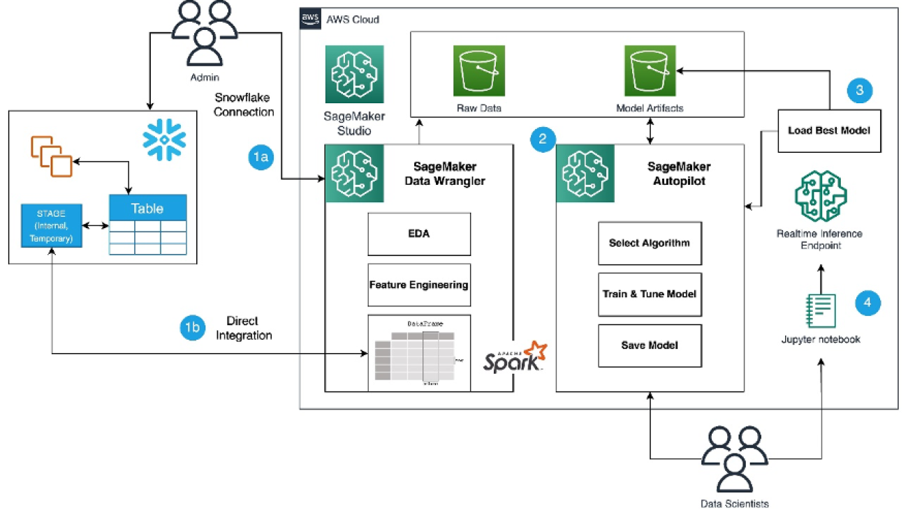
Refer to the diagram below for an overview of the low-code ML process with Snowflake, SageMaker Data Wrangler, and SageMaker Autopilot.
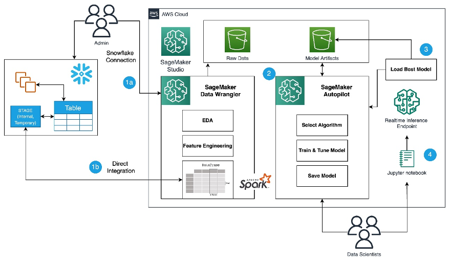
The workflow includes the following steps:
- Navigate to SageMaker Data Wrangler for your data preparation and feature engineering tasks.
- Set up the Snowflake connection with SageMaker Data Wrangler.
- Explore your Snowflake tables in SageMaker Data Wrangler, create a ML dataset, and perform feature engineering.
- Train and test the models using SageMaker Data Wrangler and SageMaker Autopilot.
- Load the best model to a real-time inference endpoint for predictions.
- Use a Python notebook to invoke the launched real-time inference endpoint.
Prerequisites
For this post, the administrator needs the following prerequisites:
- A Snowflake user with administrator permission to create a Snowflake virtual warehouse, user, and role, and grant access to this user to create a database. For more details on the administration setup, refer to Import data from Snowflake.
- An AWS account with admin access.
- A Snowflake Enterprise Account in your preferred AWS Region with
ACCOUNTADMINaccess. - Optionally, if you’re using Snowflake OAuth access in SageMaker Data Wrangler, refer to Import data from Snowflake to set up an OAuth identity provider.
- Familiarity with Snowflake, basic SQL, the Snowsight UI, and Snowflake objects.
Data scientists should have the following prerequisites
- Access to Amazon SageMaker, an instance of Amazon SageMaker Studio, and a user for SageMaker Studio. For more information about prerequisites, see Get Started with Data Wrangler.
- Familiarity with AWS services, networking, and the AWS Management Console.
Basic knowledge of Python, Jupyter notebooks, and ML.
Lastly, you should prepare your data for Snowflake
- We use credit card transaction data from Kaggle to build ML models for detecting fraudulent credit card transactions, so customers are not charged for items that they didn’t purchase. The dataset includes credit card transactions in September 2013 made by European cardholders.
- You should use the SnowSQL client and install it in your local machine, so you can use it to upload the dataset to a Snowflake table.
The following steps show how to prepare and load the dataset into the Snowflake database. This is a one-time setup.
Snowflake table and data preparation
Complete the following steps for this one-time setup:
- First, as the administrator, create a Snowflake virtual warehouse, user, and role, and grant access to other users such as the data scientists to create a database and stage data for their ML use cases:
- As the data scientist, let’s now create a database and import the credit card transactions into the Snowflake database to access the data from SageMaker Data Wrangler. For illustration purposes, we create a Snowflake database named
SF_FIN_TRANSACTION: - Download the dataset CSV file to your local machine and create a stage to load the data into the database table. Update the file path to point to the downloaded dataset location before running the PUT command for importing the data to the created stage:
- Create a table named
credit_card_transactions: - Import the data into the created table from the stage:
Set up the SageMaker Data Wrangler and Snowflake connection
After we prepare the dataset to use with SageMaker Data Wrangler, let us create a new Snowflake connection in SageMaker Data Wrangler to connect to the sf_fin_transaction database in Snowflake and query the credit_card_transaction table:
- Choose Snowflake on the SageMaker Data Wrangler Connection page.
- Provide a name to identify your connection.
- Select your authentication method to connect with the Snowflake database:
- If using basic authentication, provide the user name and password shared by your Snowflake administrator. For this post, we use basic authentication to connect to Snowflake using the user credentials we created in the previous step.
- If you are using OAuth, provide your identity provider credentials.
SageMaker Data Wrangler by default queries your data directly from Snowflake without creating any data copies in S3 buckets. SageMaker Data Wrangler’s new usability enhancement uses Apache Spark to integrate with Snowflake to prepare and seamlessly create a dataset for your ML journey.
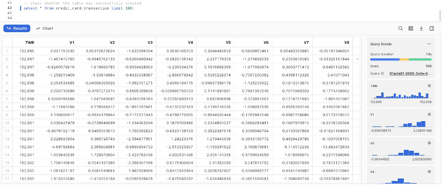
So far, we have created the database on Snowflake, imported the CSV file into the Snowflake table, created Snowflake credentials, and created a connector on SageMaker Data Wrangler to connect to Snowflake. To validate the configured Snowflake connection, run the following query on the created Snowflake table:
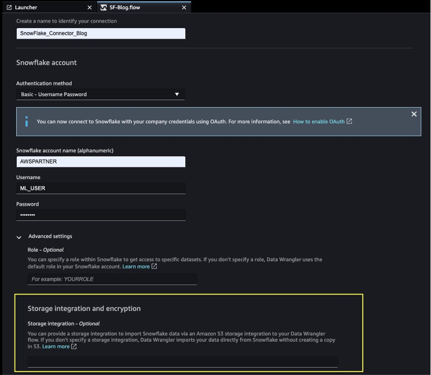
Note that the storage integration option that was required before is now optional in the advanced settings.
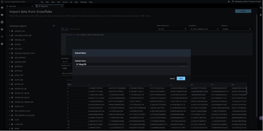
Explore Snowflake data
After you validate the query results, choose Import to save the query results as the dataset. We use this extracted dataset for exploratory data analysis and feature engineering.
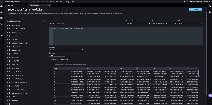
You can choose to sample the data from Snowflake in the SageMaker Data Wrangler UI. Another option is to download complete data for your ML model training use cases using SageMaker Data Wrangler processing jobs.
Perform exploratory data analysis in SageMaker Data Wrangler
The data within Data Wrangler needs to be engineered before it can be trained. In this section, we demonstrate how to perform feature engineering on the data from Snowflake using SageMaker Data Wrangler’s built-in capabilities.
First, let’s use the Data Quality and Insights Report feature within SageMaker Data Wrangler to generate reports to automatically verify the data quality and detect abnormalities in the data from Snowflake.
You can use the report to help you clean and process your data. It gives you information such as the number of missing values and the number of outliers. If you have issues with your data, such as target leakage or imbalance, the insights report can bring those issues to your attention. To understand the report details, refer to Accelerate data preparation with data quality and insights in Amazon SageMaker Data Wrangler.
After you check out the data type matching applied by SageMaker Data Wrangler, complete the following steps:
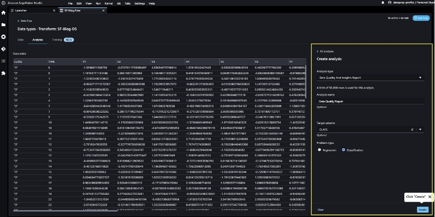
- Choose the plus sign next to Data types and choose Add analysis.
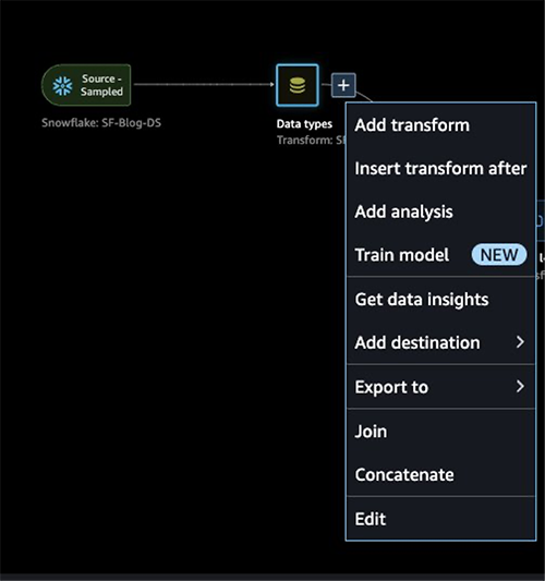
- For Analysis type, choose Data Quality and Insights Report.
- Choose Create.
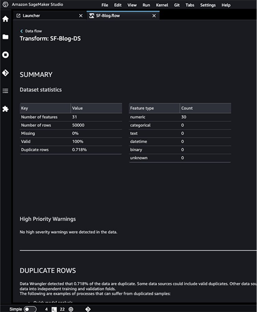
- Refer to the Data Quality and Insights Report details to check out high-priority warnings.
You can choose to resolve the warnings reported before proceeding with your ML journey.
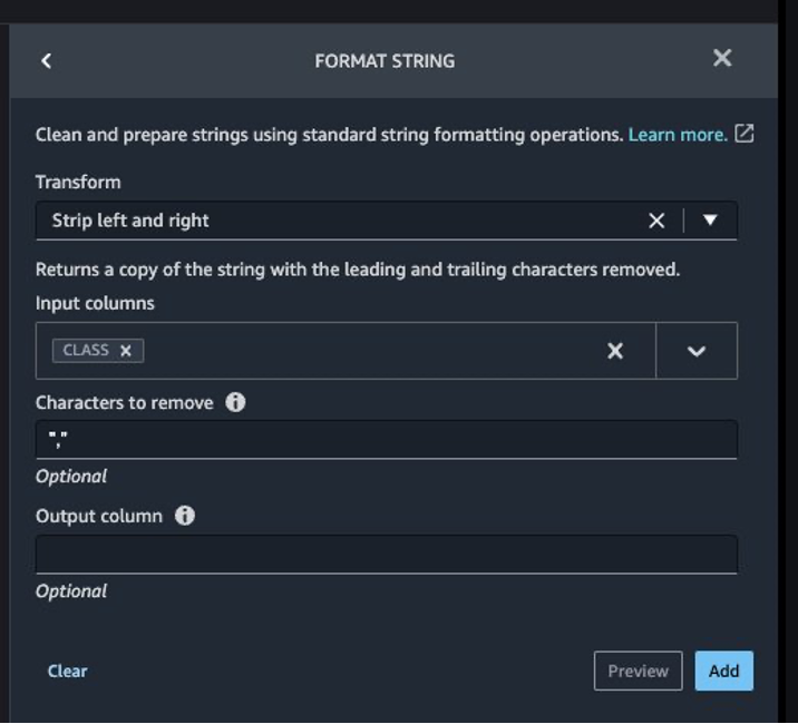
The target column Class to be predicted is classified as a string. First, let’s apply a transformation to remove the stale empty characters.
- Choose Add step and choose Format string.
- In the list of transforms, choose Strip left and right.
- Enter the characters to remove and choose Add.
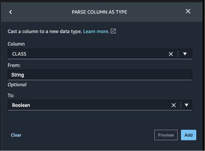
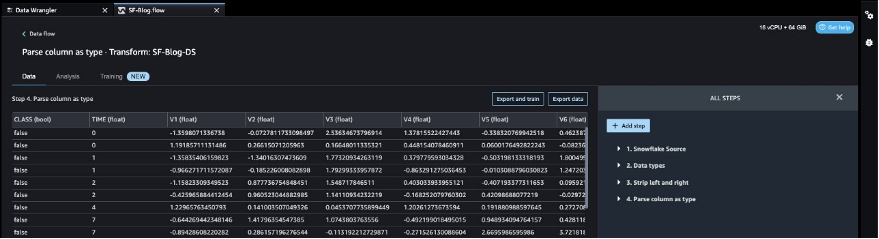
Next, we convert the target column Class from the string data type to Boolean because the transaction is either legitimate or fraudulent.
- Choose Add step.
- Choose Parse column as type.
- For Column, choose
Class. - For From, choose String.
- For To, choose Boolean.
- Choose Add.
After the target column transformation, we reduce the number of feature columns, because there are over 30 features in the original dataset. We use Principal Component Analysis (PCA) to reduce the dimensions based on feature importance. To understand more about PCA and dimensionality reduction, refer to Principal Component Analysis (PCA) Algorithm.
- Choose Add step.
- Choose Dimensionality Reduction.
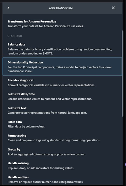
- For Transform, choose Principal component analysis.
- For Input columns, choose all the columns except the target column
Class.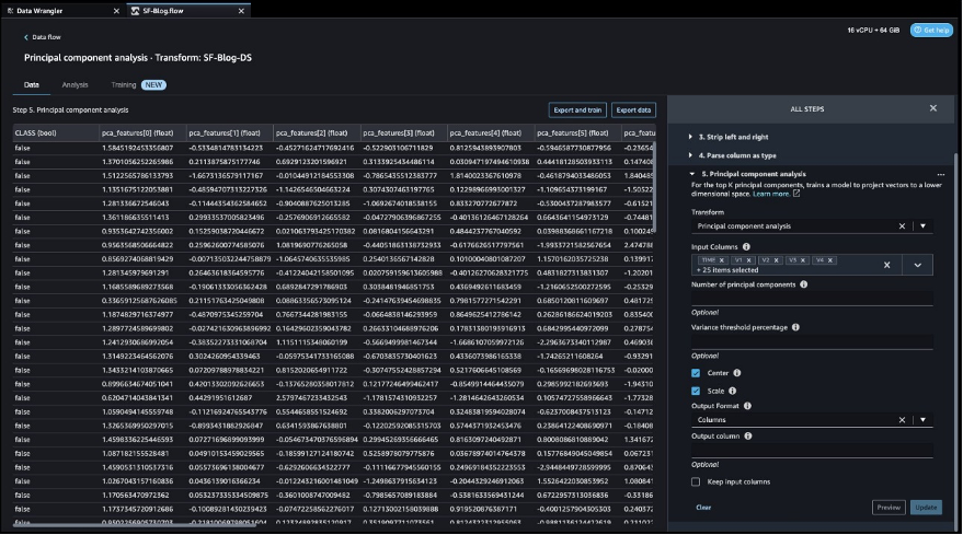
- Choose the plus sign next to Data flow and choose Add analysis.
- For Analysis type, choose Quick Model.
- For Analysis name, enter a name.
- For Label, choose
Class.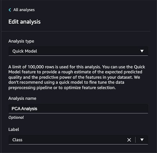
- Choose Run.
Based on the PCA results, you can decide which features to use for building the model. In the following screenshot, the graph shows the features (or dimensions) ordered based on highest to lowest importance to predict the target class, which in this dataset is whether the transaction is fraudulent or valid.
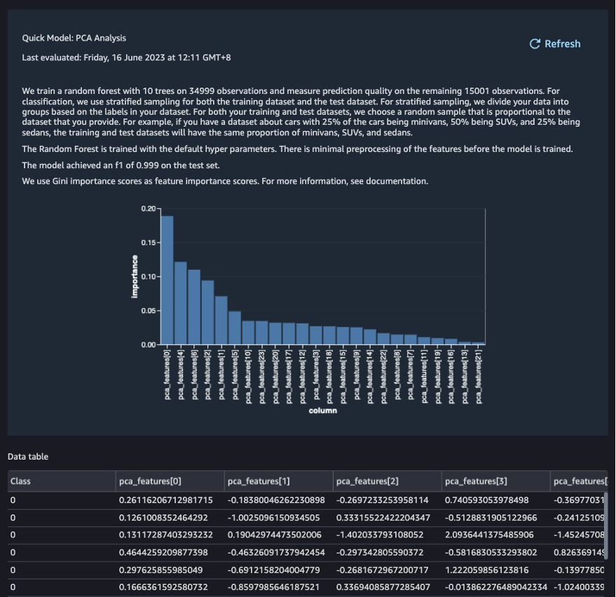
You can choose to reduce the number of features based on this analysis, but for this post, we leave the defaults as is.
This concludes our feature engineering process, although you may choose to run the quick model and create a Data Quality and Insights Report again to understand the data before performing further optimizations.
Export data and train the model
In the next step, we use SageMaker Autopilot to automatically build, train, and tune the best ML models based on your data. With SageMaker Autopilot, you still maintain full control and visibility of your data and model.
Now that we have completed the exploration and feature engineering, let’s train a model on the dataset and export the data to train the ML model using SageMaker Autopilot.
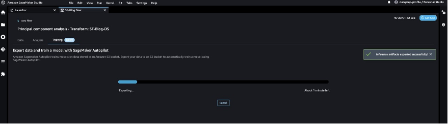
- On the Training tab, choose Export and train.
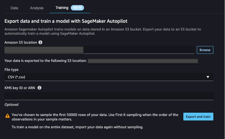
We can monitor the export progress while we wait for it to complete.
Let’s configure SageMaker Autopilot to run an automated training job by specifying the target we want to predict and the type of problem. In this case, because we’re training the dataset to predict whether the transaction is fraudulent or valid, we use binary classification.
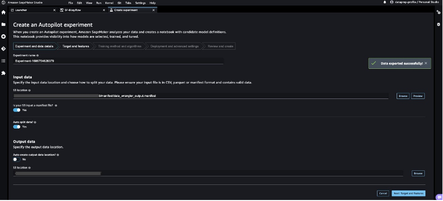
- Enter a name for your experiment, provide the S3 location data, and choose Next: Target and features.
- For Target, choose
Classas the column to predict. - Choose Next: Training method.

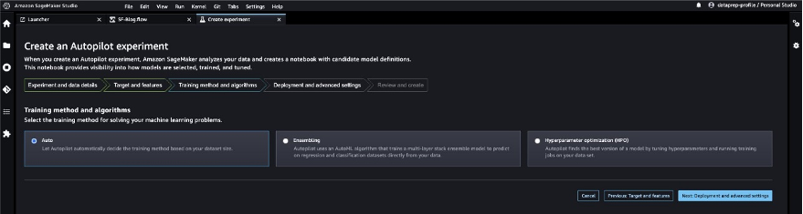
Let’s allow SageMaker Autopilot to decide the training method based on the dataset.
- For Training method and algorithms, select Auto.
To understand more about the training modes supported by SageMaker Autopilot, refer to Training modes and algorithm support.
- Choose Next: Deployment and advanced settings.
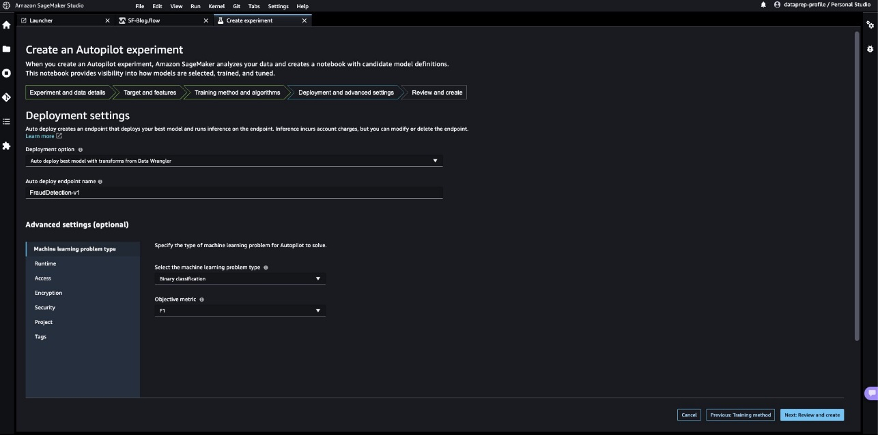
- For Deployment option, choose Auto deploy the best model with transforms from Data Wrangler, which loads the best model for inference after the experimentation is complete.
- Enter a name for your endpoint.
- For Select the machine learning problem type, choose Binary classification.
- For Objection metric, choose F1.
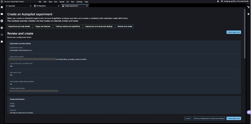
- Choose Next: Review and create.
- Choose Create experiment.
This starts an SageMaker Autopilot job that creates a set of training jobs that uses combinations of hyperparameters to optimize the objective metric.
Wait for SageMaker Autopilot to finish building the models and evaluation of the best ML model.
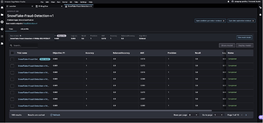
Launch a real-time inference endpoint to test the best model
SageMaker Autopilot runs experiments to determine the best model that can classify credit card transactions as legitimate or fraudulent.
When SageMaker Autopilot completes the experiment, we can view the training results with the evaluation metrics and explore the best model from the SageMaker Autopilot job description page.
- Select the best model and choose Deploy model.
We use a real-time inference endpoint to test the best model created through SageMaker Autopilot.
- Select Make real-time predictions.
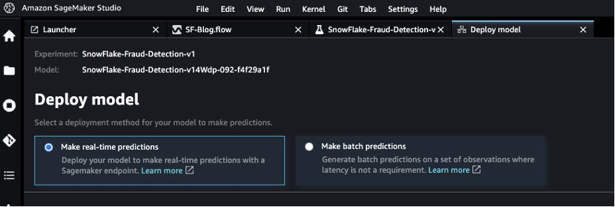
When the endpoint is available, we can pass the payload and get inference results.
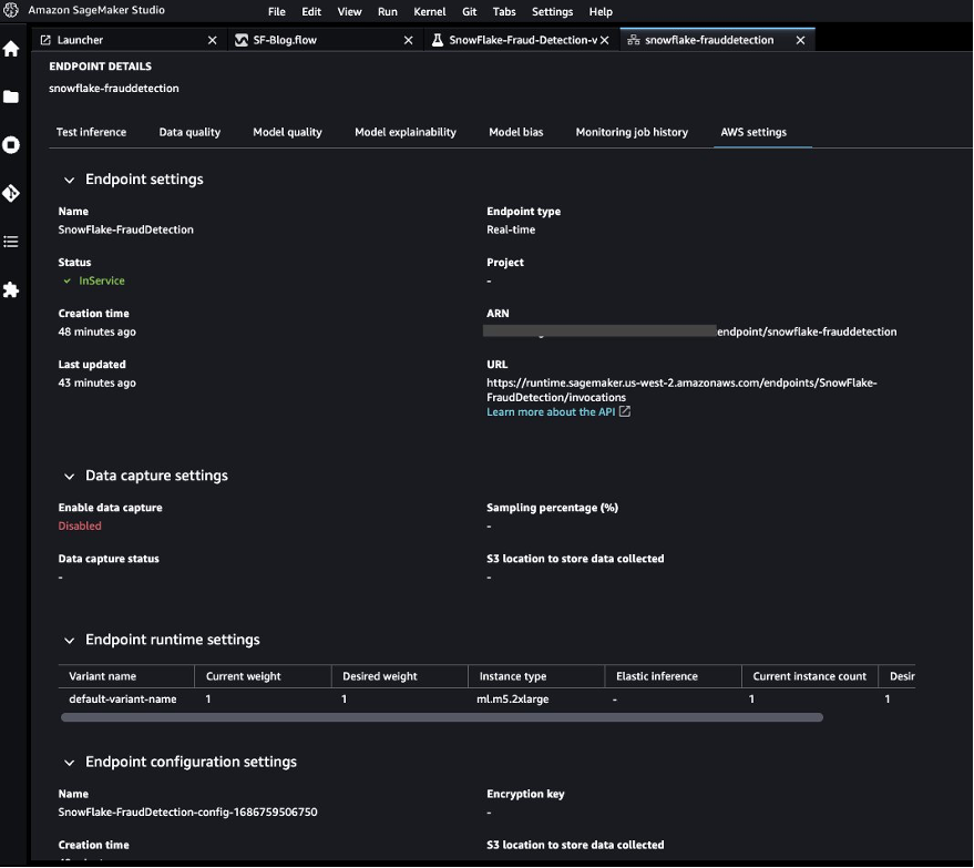
Let’s launch a Python notebook to use the inference endpoint.
- On the SageMaker Studio console, choose the folder icon in the navigation pane and choose Create notebook.
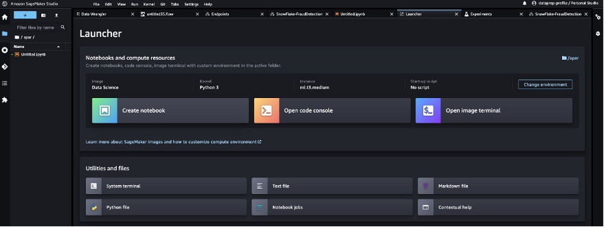
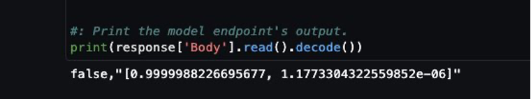
- Use the following Python code to invoke the deployed real-time inference endpoint:
The output shows the result as false, which implies the sample feature data is not fraudulent.
Clean up
To make sure you don’t incur charges after completing this tutorial, shut down the SageMaker Data Wrangler application and shut down the notebook instance used to perform inference. You should also delete the inference endpoint you created using SageMaker Autopilot to prevent additional charges.
Conclusion
In this post, we demonstrated how to bring your data from Snowflake directly without creating any intermediate copies in the process. You can either sample or load your complete dataset to SageMaker Data Wrangler directly from Snowflake. You can then explore the data, clean the data, and perform featuring engineering using SageMaker Data Wrangler’s visual interface.
We also highlighted how you can easily train and tune a model with SageMaker Autopilot directly from the SageMaker Data Wrangler user interface. With SageMaker Data Wrangler and SageMaker Autopilot integration, we can quickly build a model after completing feature engineering, without writing any code. Then we referenced SageMaker Autopilot’s best model to run inferences using a real-time endpoint.
Try out the new Snowflake direct integration with SageMaker Data Wrangler today to easily build ML models with your data using SageMaker.
About the authors
 Hariharan Suresh is a Senior Solutions Architect at AWS. He is passionate about databases, machine learning, and designing innovative solutions. Prior to joining AWS, Hariharan was a product architect, core banking implementation specialist, and developer, and worked with BFSI organizations for over 11 years. Outside of technology, he enjoys paragliding and cycling.
 Aparajithan Vaidyanathan is a Principal Enterprise Solutions Architect at AWS. He supports enterprise customers migrate and modernize their workloads on AWS cloud. He is a Cloud Architect with 23+ years of experience designing and developing enterprise, large-scale and distributed software systems. He specializes in Machine Learning & Data Analytics with focus on Data and Feature Engineering domain. He is an aspiring marathon runner and his hobbies include hiking, bike riding and spending time with his wife and two boys.
 Tim Song is a Software Development Engineer at AWS SageMaker, with 10+ years of experience as software developer, consultant and tech leader he has demonstrated ability to deliver scalable and reliable products and solve complex problems. In his spare time, he enjoys the nature, outdoor running, hiking and etc.
 Bosco Albuquerque is a Sr. Partner Solutions Architect at AWS and has over 20 years of experience in working with database and analytics products from enterprise database vendors and cloud providers. He has helped large technology companies design data analytics solutions and has led engineering teams in designing and implementing data analytics platforms and data products.
Deploy a serverless ML inference endpoint of large language models using FastAPI, AWS Lambda, and AWS CDK
For data scientists, moving machine learning (ML) models from proof of concept to production often presents a significant challenge. One of the main challenges can be deploying a well-performing, locally trained model to the cloud for inference and use in other applications. It can be cumbersome to manage the process, but with the right tool, you can significantly reduce the required effort.
Amazon SageMaker inference, which was made generally available in April 2022, makes it easy for you to deploy ML models into production to make predictions at scale, providing a broad selection of ML infrastructure and model deployment options to help meet all kinds of ML inference needs. You can use SageMaker Serverless Inference endpoints for workloads that have idle periods between traffic spurts and can tolerate cold starts. The endpoints scale out automatically based on traffic and take away the undifferentiated heavy lifting of selecting and managing servers. Additionally, you can use AWS Lambda directly to expose your models and deploy your ML applications using your preferred open-source framework, which can prove to be more flexible and cost-effective.
FastAPI is a modern, high-performance web framework for building APIs with Python. It stands out when it comes to developing serverless applications with RESTful microservices and use cases requiring ML inference at scale across multiple industries. Its ease and built-in functionalities like the automatic API documentation make it a popular choice amongst ML engineers to deploy high-performance inference APIs. You can define and organize your routes using out-of-the-box functionalities from FastAPI to scale out and handle growing business logic as needed, test locally and host it on Lambda, then expose it through a single API gateway, which allows you to bring an open-source web framework to Lambda without any heavy lifting or refactoring your codes.
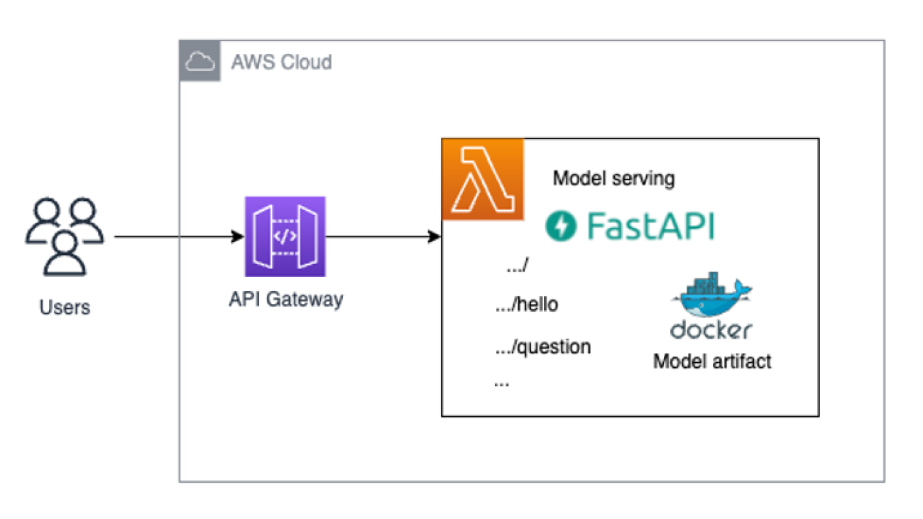
This post shows you how to easily deploy and run serverless ML inference by exposing your ML model as an endpoint using FastAPI, Docker, Lambda, and Amazon API Gateway. We also show you how to automate the deployment using the AWS Cloud Development Kit (AWS CDK).
Solution overview
The following diagram shows the architecture of the solution we deploy in this post.

Prerequisites
You must have the following prerequisites:
- Python3 installed, along with
virtualenvfor creating and managing virtual environments in Python - aws-cdk v2 installed on your system in order to be able to use the AWS CDK CLI
- Docker installed and running on your local machine
Test if all the necessary software is installed:
- The AWS Command Line Interface (AWS CLI) is needed. Log in to your account and choose the Region where you want to deploy the solution.
- Use the following code to check your Python version:
- Check if
virtualenvis installed for creating and managing virtual environments in Python. Strictly speaking, this is not a hard requirement, but it will make your life easier and helps follow along with this post more easily. Use the following code: - Check if cdk is installed. This will be used to deploy our solution.
- Check if Docker is installed. Our solution will make your model accessible through a Docker image to Lambda. To build this image locally, we need Docker.
- Make sure Docker is up and running with the following code:
How to structure your FastAPI project using AWS CDK
We use the following directory structure for our project (ignoring some boilerplate AWS CDK code that is immaterial in the context of this post):
The directory follows the recommended structure of AWS CDK projects for Python.
The most important part of this repository is the fastapi_model_serving directory. It contains the code that will define the AWS CDK stack and the resources that are going to be used for model serving.
The fastapi_model_serving directory contains the model_endpoint subdirectory, which contains all the assets necessary that make up our serverless endpoint, namely the Dockerfile to build the Docker image that Lambda will use, the Lambda function code that uses FastAPI to handle inference requests and route them to the correct endpoint, and the model artifacts of the model that we want to deploy. model_endpoint also contains the following:
Docker– This subdirectory contains the following:Dockerfile– This is used to build the image for the Lambda function with all the artifacts (Lambda function code, model artifacts, and so on) in the right place so that they can be used without issues.serving.api.tar.gz– This is a tarball that contains all the assets from the runtime folder that are necessary for building the Docker image. We discuss how to create the.tar.gzfile later in this post.runtime– This subdirectory contains the following:serving_api– The code for the Lambda function and its dependencies specified in the requirements.txt file.custom_lambda_utils– This includes an inference script that loads the necessary model artifacts so that the model can be passed to theserving_apithat will then expose it as an endpoint.
Additionally, we have the template directory, which provides a template of folder structures and files where you can define your customized codes and APIs following the sample we went through earlier. The template directory contains dummy code that you can use to create new Lambda functions:
dummy– Contains the code that implements the structure of an ordinary Lambda function using the Python runtimeapi– Contains the code that implements a Lambda function that wraps a FastAPI endpoint around an existing API gateway
Deploy the solution
By default, the code is deployed inside the eu-west-1 region. If you want to change the Region, you can change the DEPLOYMENT_REGION context variable in the cdk.json file.
Keep in mind, however, that the solution tries to deploy a Lambda function on top of the arm64 architecture, and that this feature might not be available in all Regions. In this case, you need to change the architecture parameter in the fastapi_model_serving_stack.py file, as well as the first line of the Dockerfile inside the Docker directory, to host this solution on the x86 architecture.
To deploy the solution, complete the following steps:
- Run the following command to clone the GitHub repository:
git clone https://github.com/aws-samples/lambda-serverless-inference-fastapiBecause we want to showcase that the solution can work with model artifacts that you train locally, we contain a sample model artifact of a pretrained DistilBERT model on the Hugging Face model hub for a question answering task in theserving_api.tar.gzfile. The download time can take around 3–5 minutes. Now, let’s set up the environment. - Download the pretrained model that will be deployed from the Hugging Face model hub into the
./model_endpoint/runtime/serving_api/custom_lambda_utils/model_artifactsdirectory. It also creates a virtual environment and installs all dependencies that are needed. You only need to run this command once:make prep. This command can take around 5 minutes (depending on your internet bandwidth) because it needs to download the model artifacts. - Package the model artifacts inside a
.tar.gzarchive that will be used inside the Docker image that is built in the AWS CDK stack. You need to run this code whenever you make changes to the model artifacts or the API itself to always have the most up-to-date version of your serving endpoint packaged:make package_model. The artifacts are all in place. Now we can deploy the AWS CDK stack to your AWS account. - Run cdk bootstrap if it’s your first time deploying an AWS CDK app into an environment (account + Region combination):
This stack includes resources that are needed for the toolkit’s operation. For example, the stack includes an Amazon Simple Storage Service (Amazon S3) bucket that is used to store templates and assets during the deployment process.
Because we’re building Docker images locally in this AWS CDK deployment, we need to ensure that the Docker daemon is running before we can deploy this stack via the AWS CDK CLI.
- To check whether or not the Docker daemon is running on your system, use the following command:
If you don’t get an error message, you should be ready to deploy the solution.
- Deploy the solution with the following command:
This step can take around 5–10 minutes due to building and pushing the Docker image.
Troubleshooting
If you’re a Mac user, you may encounter an error when logging into Amazon Elastic Container Registry (Amazon ECR) with the Docker login, such as Error saving credentials ... not implemented. For example:
Before you can use Lambda on top of Docker containers inside the AWS CDK, you may need to change the ~/docker/config.json file. More specifically, you might have to change the credsStore parameter in ~/.docker/config.json to osxkeychain. That solves Amazon ECR login issues on a Mac.
Run real-time inference
After your AWS CloudFormation stack is deployed successfully, go to the Outputs tab for your stack on the AWS CloudFormation console and open the endpoint URL. Now our model is accessible via the endpoint URL and we’re ready to run real-time inference.
Navigate to the URL to see if you can see “hello world” message and add /docs to the address to see if you can see the interactive swagger UI page successfully. There might be some cold start time, so you may need to wait or refresh a few times.

After you log in to the landing page of the FastAPI swagger UI page, you can run via the root / or via /question.
From /, you could run the API and get the “hello world” message.
From /question, you could run the API and run ML inference on the model we deployed for a question answering case. For example, we use the question is What is the color of my car now? and the context is My car used to be blue but I painted red.

When you choose Execute, based on the given context, the model will answer the question with a response, as shown in the following screenshot.

In the response body, you can see the answer with the confidence score from the model. You could also experiment with other examples or embed the API in your existing application.
Alternatively, you can run the inference via code. Here is one example written in Python, using the requests library:
The code outputs a string similar to the following:
If you are interested in knowing more about deploying Generative AI and large language models on AWS, check out here:
- Deploy Serverless Generative AI on AWS Lambda with OpenLLaMa
- Deploy large language models on AWS Inferentia2 using large model inference containers
Clean up
Inside the root directory of your repository, run the following code to clean up your resources:
Conclusion
In this post, we introduced how you can use Lambda to deploy your trained ML model using your preferred web application framework, such as FastAPI. We provided a detailed code repository that you can deploy, and you retain the flexibility of switching to whichever trained model artifacts you process. The performance can depend on how you implement and deploy the model.
You are welcome to try it out yourself, and we’re excited to hear your feedback!
About the Authors
 Tingyi Li is an Enterprise Solutions Architect from AWS based out in Stockholm, Sweden supporting the Nordics customers. She enjoys helping customers with the architecture, design, and development of cloud-optimized infrastructure solutions. She is specialized in AI and Machine Learning and is interested in empowering customers with intelligence in their AI/ML applications. In her spare time, she is also a part-time illustrator who writes novels and plays the piano.
 Demir Catovic is a Machine Learning Engineer from AWS based in Zurich, Switzerland. He engages with customers and helps them implement scalable and fully-functional ML applications. He is passionate about building and productionizing machine learning applications for customers and is always keen to explore around new trends and cutting-edge technologies in the AI/ML world.
How Light & Wonder built a predictive maintenance solution for gaming machines on AWS
This post is co-written with Aruna Abeyakoon and Denisse Colin from Light and Wonder (L&W).
Headquartered in Las Vegas, Light & Wonder, Inc. is the leading cross-platform global game company that provides gambling products and services. Working with AWS, Light & Wonder recently developed an industry-first secure solution, Light & Wonder Connect (LnW Connect), to stream telemetry and machine health data from roughly half a million electronic gaming machines distributed across its casino customer base globally when LnW Connect reaches its full potential. Over 500 machine events are monitored in near-real time to give a full picture of machine conditions and their operating environments. Utilizing data streamed through LnW Connect, L&W aims to create better gaming experience for their end-users as well as bring more value to their casino customers.
Light & Wonder teamed up with the Amazon ML Solutions Lab to use events data streamed from LnW Connect to enable machine learning (ML)-powered predictive maintenance for slot machines. Predictive maintenance is a common ML use case for businesses with physical equipment or machinery assets. With predictive maintenance, L&W can get advanced warning of machine breakdowns and proactively dispatch a service team to inspect the issue. This will reduce machine downtime and avoid significant revenue loss for casinos. With no remote diagnostic system in place, issue resolution by the Light & Wonder service team on the casino floor can be costly and inefficient, while severely degrading the customer gaming experience.
The nature of the project is highly exploratory—this is the first attempt at predictive maintenance in the gaming industry. The Amazon ML Solutions Lab and L&W team embarked on an end-to-end journey from formulating the ML problem and defining the evaluation metrics, to delivering a high-quality solution. The final ML model combines CNN and Transformer, which are the state-of-the-art neural network architectures for modeling sequential machine log data. The post presents a detailed description of this journey, and we hope you will enjoy it as much as we do!
In this post, we discuss the following:
- How we formulated the predictive maintenance problem as an ML problem with a set of appropriate metrics for evaluation
- How we prepared data for training and testing
- Data preprocessing and feature engineering techniques we employed to obtain performant models
- Performing a hyperparameter tuning step with Amazon SageMaker Automatic Model Tuning
- Comparisons between the baseline model and the final CNN+Transformer model
- Additional techniques we used to improve model performance, such as ensembling
Background
In this section, we discuss the issues that necessitated this solution.
Dataset
Slot machine environments are highly regulated and are deployed in an air-gapped environment. In LnW Connect, an encryption process was designed to provide a secure and reliable mechanism for the data to be brought into an AWS data lake for predictive modeling. The aggregated files are encrypted and the decryption key is only available in AWS Key Management Service (AWS KMS). A cellular-based private network into AWS is set up through which the files were uploaded into Amazon Simple Storage Service (Amazon S3).
LnW Connect streams a wide range of machine events, such as start of game, end of game, and more. The system collects over 500 different types of events. As shown in the following
, each event is recorded along with a timestamp of when it happened and the ID of the machine recording the event. LnW Connect also records when a machine enters a non-playable state, and it will be marked as a machine failure or breakdown if it doesn’t recover to a playable state within a sufficiently short time span.
| Machine ID | Event Type ID | Timestamp |
|---|---|---|
| 0 | E1 | 2022-01-01 00:17:24 |
| 0 | E3 | 2022-01-01 00:17:29 |
| 1000 | E4 | 2022-01-01 00:17:33 |
| 114 | E234 | 2022-01-01 00:17:34 |
| 222 | E100 | 2022-01-01 00:17:37 |
In addition to dynamic machine events, static metadata about each machine is also available. This includes information such as machine unique identifier, cabinet type, location, operating system, software version, game theme, and more, as shown in the following table. (All the names in the table are anonymized to protect customer information.)
| Machine ID | Cabinet Type | OS | Location | Game Theme |
|---|---|---|---|---|
| 276 | A | OS_Ver0 | AA Resort & Casino | StormMaiden |
| 167 | B | OS_Ver1 | BB Casino, Resort & Spa | UHMLIndia |
| 13 | C | OS_Ver0 | CC Casino & Hotel | TerrificTiger |
| 307 | D | OS_Ver0 | DD Casino Resort | NeptunesRealm |
| 70 | E | OS_Ver0 | EE Resort & Casino | RLPMealTicket |
Problem definition
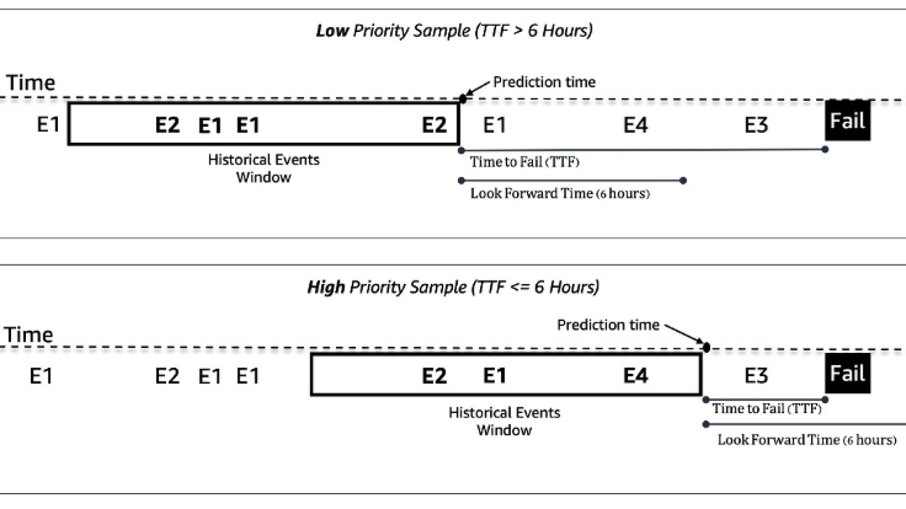
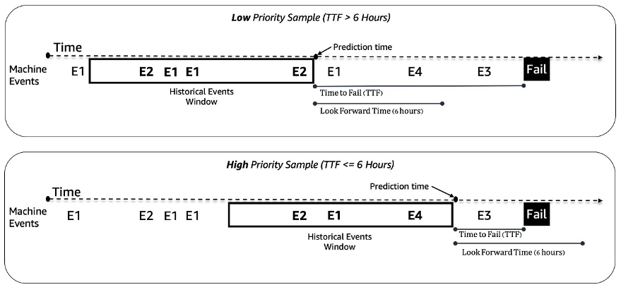
We treat the predictive maintenance problem for slot machines as a binary classification problem. The ML model takes in the historical sequence of machine events and other metadata and predicts whether a machine will encounter a failure in a 6-hour future time window. If a machine will break down within 6 hours, it is deemed a high-priority machine for maintenance. Otherwise, it is low priority. The following figure gives examples of low-priority (top) and high-priority (bottom) samples. We use a fixed-length look-back time window to collect historical machine event data for prediction. Experiments show that longer look-back time windows improve model performance significantly (more details later in this post).
Modeling challenges
We faced a couple of challenges solving this problem:
- We have a huge amount event logs that contain around 50 million events a month (from approximately 1,000 game samples). Careful optimization is needed in the data extraction and preprocessing stage.
- Event sequence modeling was challenging due to the extremely uneven distribution of events over time. A 3-hour window can contain anywhere from tens to thousands of events.
- Machines are in a good state most of the time and the high-priority maintenance is a rare class, which introduced a class imbalance issue.
- New machines are added continuously to the system, so we had to make sure our model can handle prediction on new machines that have never been seen in training.
Data preprocessing and feature engineering
In this section, we discuss our methods for data preparation and feature engineering.
Feature engineering
Slot machine feeds are streams of unequally spaced time series events; for example, the number of events in a 3-hour window can range from tens to thousands. To handle this imbalance, we used event frequencies instead of the raw sequence data. A straightforward approach is aggregating the event frequency for the entire look-back window and feeding it into the model. However, when using this representation, the temporal information is lost, and the order of events is not preserved. We instead used temporal binning by dividing the time window into N equal sub-windows and calculating the event frequencies in each. The final features of a time window are the concatenation of all its sub-window features. Increasing the number of bins preserves more temporal information. The following figure illustrates temporal binning on a sample window.

First, the sample time window is split into two equal sub-windows (bins); we used only two bins here for simplicity for illustration. Then, the counts of the events E1, E2, E3, and E4 are calculated in each bin. Lastly, they are concatenated and used as features.
Along with the event frequency-based features, we used machine-specific features like software version, cabinet type, game theme, and game version. Additionally, we added features related to the timestamps to capture the seasonality, such as hour of the day and day of the week.
Data preparation
To extract data efficiently for training and testing, we utilize Amazon Athena and the AWS Glue Data Catalog. The events data is stored in Amazon S3 in Parquet format and partitioned according to day/month/hour. This facilitates efficient extraction of data samples within a specified time window. We use data from all machines in the latest month for testing and the rest of the data for training, which helps avoid potential data leakage.
ML methodology and model training
In this section, we discuss our baseline model with AutoGluon and how we built a customized neural network with SageMaker automatic model tuning.
Building a baseline model with AutoGluon
With any ML use case, it’s important to establish a baseline model to be used for comparison and iteration. We used AutoGluon to explore several classic ML algorithms. AutoGluon is easy-to-use AutoML tool that uses automatic data processing, hyperparameter tuning, and model ensemble. The best baseline was achieved with a weighted ensemble of gradient boosted decision tree models. The ease of use of AutoGluon helped us in the discovery stage to navigate quickly and efficiently through a wide range of possible data and ML modeling directions.
Building and tuning a customized neural network model with SageMaker automatic model tuning
After experimenting with different neural networks architectures, we built a customized deep learning model for predictive maintenance. Our model surpassed the AutoGluon baseline model by 121% in recall at 80% precision. The final model ingests historical machine event sequence data, time features such as hour of the day, and static machine metadata. We utilize SageMaker automatic model tuning jobs to search for the best hyperparameters and model architectures.
The following figure shows the model architecture. We first normalize the binned event sequence data by average frequencies of each event in the training set to remove the overwhelming effect of high-frequency events (start of game, end of game, and so on). The embeddings for individual events are learnable, while the temporal feature embeddings (day of the week, hour of the day) are extracted using the package GluonTS. Then we concatenate the event sequence data with the temporal feature embeddings as the input to the model. The model consists of the following layers:
- Convolutional layers (CNN) – Each CNN layer consists of two 1-dimensional convolutional operations with residual connections. The output of each CNN layer has the same sequence length as the input to allow for easy stacking with other modules. The total number of CNN layers is a tunable hyperparameter.
- Transformer encoder layers (TRANS) – The output of the CNN layers is fed together with the positional encoding to a multi-head self-attention structure. We use TRANS to directly capture temporal dependencies instead of using recurrent neural networks. Here, binning of the raw sequence data (reducing length from thousands to hundreds) helps alleviate the GPU memory bottlenecks, while keeping the chronological information to a tunable extent (the number of the bins is a tunable hyperparameter).
- Aggregation layers (AGG) – The final layer combines the metadata information (game theme type, cabinet type, locations) to produce the priority level probability prediction. It consists of several pooling layers and fully connected layers for incremental dimension reduction. The multi-hot embeddings of metadata are also learnable, and don’t go through CNN and TRANS layers because they don’t contain sequential information.

We use the cross-entropy loss with class weights as tunable hyperparameters to adjust for the class imbalance issue. In addition, the numbers of CNN and TRANS layers are crucial hyperparameters with the possible values of 0, which means specific layers may not always exist in the model architecture. This way, we have a unified framework where the model architectures are searched along with other usual hyperparameters.
We utilize SageMaker automatic model tuning, also known as hyperparameter optimization (HPO), to efficiently explore model variations and the large search space of all hyperparameters. Automatic model tuning receives the customized algorithm, training data, and hyperparameter search space configurations, and searches for best hyperparameters using different strategies such as Bayesian, Hyperband, and more with multiple GPU instances in parallel. After evaluating on a hold-out validation set, we obtained the best model architecture with two layers of CNN, one layer of TRANS with four heads, and an AGG layer.
We used the following hyperparameter ranges to search for the best model architecture:
To further improve model accuracy and reduce model variance, we trained the model with multiple independent random weight initializations, and aggregated the result with mean values as the final probability prediction. There is a trade-off between more computing resources and better model performance, and we observed that 5–10 should be a reasonable number in the current use case (results shown later in this post).
Model performance results
In this section, we present the model performance evaluation metrics and results.
Evaluation metrics
Precision is very important for this predictive maintenance use case. Low precision means reporting more false maintenance calls, which drives costs up through unnecessary maintenance. Because average precision (AP) doesn’t fully align with the high precision objective, we introduced a new metric named average recall at high precisions (ARHP). ARHP is equal to the average of recalls at 60%, 70%, and 80% precision points. We also used precision at top K% (K=1, 10), AUPR, and AUROC as additional metrics.
Results
The following table summarizes the results using the baseline and the customized neural network models, with 7/1/2022 as the train/test split point. Experiments show that increasing the window length and sample data size both improve the model performance, because they contain more historical information to help with the prediction. Regardless of the data settings, the neural network model outperforms AutoGluon in all metrics. For example, recall at the fixed 80% precision is increased by 121%, which enables you to quickly identify more malfunctioned machines if using the neural network model.
| Model | Window length/Data size | AUROC | AUPR | ARHP | Recall@Prec0.6 | Recall@Prec0.7 | Recall@Prec0.8 | Prec@top1% | Prec@top10% |
|---|---|---|---|---|---|---|---|---|---|
| AutoGluon baseline | 12H/500k | 66.5 | 36.1 | 9.5 | 12.7 | 9.3 | 6.5 | 85 | 42 |
| Neural Network | 12H/500k | 74.7 | 46.5 | 18.5 | 25 | 18.1 | 12.3 | 89 | 55 |
| AutoGluon baseline | 48H/1mm | 70.2 | 44.9 | 18.8 | 26.5 | 18.4 | 11.5 | 92 | 55 |
| Neural Network | 48H/1mm | 75.2 | 53.1 | 32.4 | 39.3 | 32.6 | 25.4 | 94 | 65 |
The following figures illustrate the effect of using ensembles to boost the neural network model performance. All the evaluation metrics shown on the x-axis are improved, with higher mean (more accurate) and lower variance (more stable). Each box-plot is from 12 repeated experiments, from no ensembles to 10 models in ensembles (x-axis). Similar trends persist in all metrics besides the Prec@top1% and Recall@Prec80% shown.
After factoring in the computational cost, we observe that using 5–10 models in ensembles is suitable for Light & Wonder datasets.
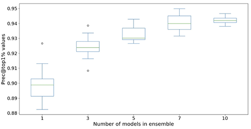
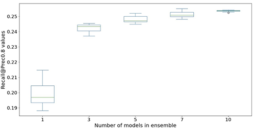
Conclusion
Our collaboration has resulted in the creation of a groundbreaking predictive maintenance solution for the gaming industry, as well as a reusable framework that could be utilized in a variety of predictive maintenance scenarios. The adoption of AWS technologies such as SageMaker automatic model tuning facilitates Light & Wonder to navigate new opportunities using near-real-time data streams. Light & Wonder is starting the deployment on AWS.
If you would like help accelerating the use of ML in your products and services, please contact the Amazon ML Solutions Lab program.
About the authors
 Aruna Abeyakoon is the Senior Director of Data Science & Analytics at Light & Wonder Land-based Gaming Division. Aruna leads the industry-first Light & Wonder Connect initiative and supports both casino partners and internal stakeholders with consumer behavior and product insights to make better games, optimize product offerings, manage assets, and health monitoring & predictive maintenance.
 Denisse Colin is a Senior Data Science Manager at Light & Wonder, a leading cross-platform global game company. She is a member of the Gaming Data & Analytics team helping develop innovative solutions to improve product performance and customers’ experiences through Light & Wonder Connect.
 Tesfagabir Meharizghi is a Data Scientist at the Amazon ML Solutions Lab where he helps AWS customers across various industries such as gaming, healthcare and life sciences, manufacturing, automotive, and sports and media, accelerate their use of machine learning and AWS cloud services to solve their business challenges.
 Mohamad Aljazaery is an applied scientist at Amazon ML Solutions Lab. He helps AWS customers identify and build ML solutions to address their business challenges in areas such as logistics, personalization and recommendations, computer vision, fraud prevention, forecasting and supply chain optimization.
 Yawei Wang is an Applied Scientist at the Amazon ML Solution Lab. He helps AWS business partners identify and build ML solutions to address their organization’s business challenges in a real-world scenario.
 Yun Zhou is an Applied Scientist at the Amazon ML Solutions Lab, where he helps with research and development to ensure the success of AWS customers. He works on pioneering solutions for various industries using statistical modeling and machine learning techniques. His interest includes generative models and sequential data modeling.
 Panpan Xu is a Applied Science Manager with the Amazon ML Solutions Lab at AWS. She is working on research and development of Machine Learning algorithms for high-impact customer applications in a variety of industrial verticals to accelerate their AI and cloud adoption. Her research interest includes model interpretability, causal analysis, human-in-the-loop AI and interactive data visualization.
 Raj Salvaji leads Solutions Architecture in the Hospitality segment at AWS. He works with hospitality customers by providing strategic guidance, technical expertise to create solutions to complex business challenges. He draws on 25 years of experience in multiple engineering roles across Hospitality, Finance and Automotive industries.
 Shane Rai is a Principal ML Strategist with the Amazon ML Solutions Lab at AWS. He works with customers across a diverse spectrum of industries to solve their most pressing and innovative business needs using AWS’s breadth of cloud-based AI/ML services.
Yash Kanoria wins SIGecom Test of Time Award
Kanoria and coauthors honored for their paper narrowing the gap between theoretical understanding and practical experience in matching markets.Read More