This post was co-written with Varun Kumar from Tealium
Retrieval Augmented Generation (RAG) pipelines are popular for generating domain-specific outputs based on external data that’s fed in as part of the context. However, there are challenges with evaluating and improving such systems. Two open-source libraries, Ragas (a library for RAG evaluation) and Auto-Instruct, used Amazon Bedrock to power a framework that evaluates and improves upon RAG.
In this post, we illustrate the importance of generative AI in the collaboration between Tealium and the AWS Generative AI Innovation Center (GenAIIC) team by automating the following:
- Evaluating the retriever and the generated answer of a RAG system based on the Ragas Repository powered by Amazon Bedrock.
- Generating improved instructions for each question-and-answer pair using an automatic prompt engineering technique based on the Auto-Instruct Repository. An instruction refers to a general direction or command given to the model to guide generation of a response. These instructions were generated using Anthropic’s Claude on Amazon Bedrock.
- Providing a UI for a human-based feedback mechanism that complements an evaluation system powered by Amazon Bedrock.
Amazon Bedrock is a fully managed service that makes popular FMs available through an API, so you can choose from a wide range of foundational models (FMs) to find the model that’s best suited for your use case. Because Amazon Bedrock is serverless, you can get started quickly, privately customize FMs with your own data, and integrate and deploy them into your applications without having to manage any infrastructure.
Tealium background and use case
Tealium is a leader in real-time customer data integration and management. They empower organizations to build a complete infrastructure for collecting, managing, and activating customer data across channels and systems. Tealium uses AI capabilities to integrate data and derive customer insights at scale. Their AI vision is to provide their customers with an active system that continuously learns from customer behaviors and optimizes engagement in real time.
Tealium has built a question and answer (QA) bot using a RAG pipeline to help identify common issues and answer questions about using the platform. The bot is expected to act as a virtual assistant to answer common questions, identify and solve issues, monitor platform health, and provide best practice suggestions, all aimed at helping Tealium customers get the most value from their customer data platform.
The primary goal of this solution with Tealium was to evaluate and improve the RAG solution that Tealium uses to power their QA bot. This was achieved by building an:
- Evaluation pipeline.
- Error correction mechanism to semi-automatically improve upon the metrics generated from evaluation. In this engagement, automatic prompt engineering was the only technique used, but others such as different chunking strategies and using semantic instead of hybrid search can be explored depending on your use case.
- A human-in the-loop feedback system allowing the human to approve or disapprove RAG outputs
Amazon Bedrock was vital in powering an evaluation pipeline and error correction mechanism because of its flexibility in choosing a wide range of leading FMs and its ability to customize models for various tasks. This allowed for testing of many types of specialized models on specific data to power such frameworks. The value of Amazon Bedrock in text generation for automatic prompt engineering and text summarization for evaluation helped tremendously in the collaboration with Tealium. Lastly, Amazon Bedrock allowed for more secure generative AI applications, giving Tealium full control over their data while also encrypting it at rest and in transit.
Solution prerequisites
To test the Tealium solution, start with the following:
- Get access to an AWS account.
- Create a SageMaker domain instance.
- Obtain access to the following models on Amazon Bedrock: Anthropic’s Claude Instant, Claude v2, Claude 3 Haiku, and Titan Embeddings G1 – Text. The evaluation using Ragas can be performed using any foundation model (FM) that’s available on Amazon Bedrock. Automatic prompt engineering must use Anthropic’s Claude v2, v2.1, or Claude Instant.
- Obtain a golden set of question and answer pairs. Specifically, you need to provide examples of questions that you will ask the RAG bot and their expected ground truths.
- Clone automatic prompt engineering and human-in-the-loop repositories. If you want access to a Ragas repository with prompts favorable towards Anthropic Claude models available on Amazon Bedrock, clone and navigate through this repository and this notebook.
The code repositories allow for flexibility of various FMs and customized models with minimal updates, illustrating Amazon Bedrock’s value in this engagement.
Solution overview
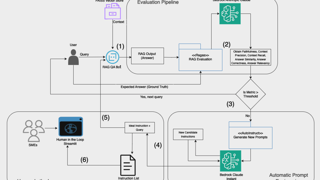
The following diagram illustrates a sample solution architecture that includes an evaluation framework, error correction technique (Auto-Instruct and automatic prompt engineering), and human-in-the-loop. As you can see, generative AI is an important part of the evaluation pipeline and the automatic prompt engineering pipeline.

The workflow consists of the following steps:
- You first enter a query into the Tealium RAG QA bot. The RAG solution uses FAISS to retrieve an appropriate context for the specified query. Then, it outputs a response.
- Ragas takes in this query, context, answer, and a ground truth that you input, and calculates faithfulness, context precision, context recall, answer correctness, answer relevancy, and answer similarity. Ragas can be integrated with Amazon Bedrock (look at the Ragas section of the notebook link). This illustrates integrating Amazon Bedrock in different frameworks.
- If any of the metrics are below a certain threshold, the specific question and answer pair is run by the Auto-Instruct library, which generates candidate instructions using Amazon Bedrock. Various FMs can be used for this text generation use case.
- The new instructions are appended to the original query to be prepared to be run by the Tealium RAG QA bot.
- The QA bot runs an evaluation to determine whether improvements have been made. Steps 3 and 4 can be iterated until all metrics are above a certain threshold. In addition, you can set a maximum number of times steps 3 and 4 are iterated to prevent an infinite loop.
- A human-in-the-loop UI is used to allow a subject matter expert (SME) to provide their own evaluation on given model outputs. This can also be used to provide guard rails against a system powered by generative AI.
In the following sections, we discuss how an example question, its context, its answer (RAG output) and ground truth (expected answer) can be evaluated and revised for a more ideal output. The evaluation is done using Ragas, a RAG evaluation library. Then, prompts and instructions are automatically generated based on their relevance to the question and answer. Lastly, you can approve or disapprove the RAG outputs based on the specific instruction generated from the automatic prompt engineering step.
Out-of-scope
Error correction and human-in-the-loop are two important aspects in this post. However, for each component, the following is out-of-scope, but can be improved upon in future iterations of the solution:
Error correction mechanism
- Automatic prompt engineering is the only method used to correct the RAG solution. This engagement didn’t go over other techniques to improve the RAG solution; such as using Amazon Bedrock to find optimal chunking strategies, vector stores, models, semantic or hybrid search, and other mechanisms. Further testing needs to be done to evaluate whether FMs from Amazon Bedrock can be a good decision maker for such parameters of a RAG solution.
- Based on the technique presented for automatic prompt engineering, there might be opportunities to optimize the cost. This wasn’t analyzed during the engagement. Disclaimer: The technique described in this post might not be the most optimal approach in terms of cost.
Human-in-the-loop
- SMEs provide their evaluation of the RAG solution by approving and disapproving FM outputs. This feedback is stored in the user’s file directory. There is an opportunity to improve upon the model based on this feedback, but this isn’t touched upon in this post.
Ragas – Evaluation of RAG pipelines
Ragas is a framework that helps evaluate a RAG pipeline. In general, RAG is a natural language processing technique that uses external data to augment an FM’s context. Therefore, this framework evaluates the ability for the bot to retrieve relevant context as well as output an accurate response to a given question. The collaboration between the AWS GenAIIC and the Tealium team showed the success of Amazon Bedrock integration with Ragas with minimal changes.
The inputs to Ragas include a set of questions, ground truths, answers, and contexts. For each question, an expected answer (ground truth), LLM output (answer), and a list of contexts (retrieved chunks) were inputted. Context recall, precision, answer relevancy, faithfulness, answer similarity, and answer correctness were evaluated using Anthropic’s Claude on Amazon Bedrock (any version). For your reference, here are the metrics that have been successfully calculated using Amazon Bedrock:
- Faithfulness – This measures the factual consistency of the generated answer against the given context, so it requires the answer and retrieved context as an input. This is a two-step prompt where the generated answer is first broken down into multiple standalone statements and propositions. Then, the evaluation LLM validates the attribution of the generated statement to the context. If the attribution can’t be validated, it’s assumed that the statement is at risk of hallucination. The answer is scaled to a 0–1 range; the higher the better.
- Context precision – This evaluates the relevancy of the context to the answer, or in other words, the retriever’s ability to capture the best context to answer your query. An LLM verifies if the information in the given context is directly relevant to the question with a single “Yes” or “No” response. The context is passed in as a list, so if the list is size one (one chunk), then the metric for context precision is either 0 (representing the context isn’t relevant to the question) or 1 (representing that it is relevant). If the context list is greater than one (or includes multiple chunks), then context precision is between 0–1, representing a specific weighted average precision calculation. This involves the context precision of the first chunk being weighted heavier than the second chunk, which itself is weighted heavier than the third chunk, and onwards, taking into account the ordering of the chunks being outputted as contexts.
- Context recall – This measures the alignment between the context and the expected RAG output, the ground truth. Similar to faithfulness, each statement in the ground truth is checked to see if it is attributed to the context (thereby evaluating the context).
- Answer similarity – This assesses the semantic similarity between the RAG output (answer) and expected answer (ground truth), with a range between 0–1. A higher score signifies better performance. First, the embeddings of answer and ground truth are created, and then a score between 0–1 is predicted, representing the semantic similarity of the embeddings using a cross encoder Tiny BERT model.
- Answer relevance – This focuses on how pertinent the generated RAG output (answer) is to the question. A lower score is assigned to answers that are incomplete or contain redundant information. To calculate this score, the LLM is asked to generate multiple questions from a given answer. Then using an Amazon Titan Embeddings model, embeddings are generated for the generated question and the actual question. The metric therefore is the mean cosine similarity between all the generated questions and the actual question.
- Answer correctness – This is the accuracy between the generated answer and the ground truth. This is calculated from the semantic similarity metric between the answer and the ground truth in addition to a factual similarity by looking at the context. A threshold value is used if you want to employ a binary 0 or 1 answer correctness score, otherwise a value between 0–1 is generated.
AutoPrompt – Automatically generate instructions for RAG
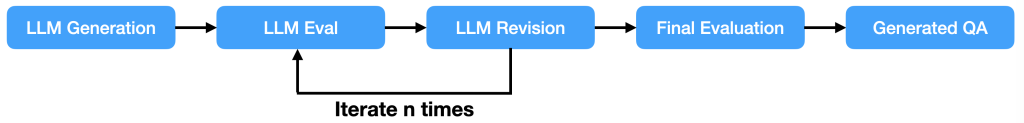
Secondly, generative AI services were shown to successfully generate and select instructions for prompting FMs. In a nutshell, instructions are generated by an FM that best map a question and context to the RAG QA bot answer based on a certain style. This process was done using the Auto-Instruct library. The approach harnesses the ability of FMs to produce candidate instructions, which are then ranked using a scoring model to determine the most effective prompts.
First, you need to ask an Anthropic’s Claude model on Amazon Bedrock to generate an instruction for a set of inputs (question and context) that map to an output (answer). The FM is then asked to generate a specific type of instruction, such as a one-paragraph instruction, one-sentence instruction, or step-by-step instruction. Many candidate instructions are then generated. Look at the generate_candidate_prompts() function to see the logic in code.
Then, the resulting candidate instructions are tested against each other using an evaluation FM. To do this, first, each instruction is compared against all other instructions. Then, the evaluation FM is used to evaluate the quality of the prompts for a given task (query plus context to answer pairs). The evaluation logic for a sample pair of candidate instructions is shown in the test_candidate_prompts() function.
This outputs the most ideal prompt generated by the framework. For each question-and-answer pair, the output includes the best instruction, second best instruction, and third best instruction.
For a demonstration of performing automatic prompt engineering (and calling Ragas):
- Navigate through the following notebook.
- Code snippets for how candidate prompts are generated and evaluated are included in this source file with their associated prompts included in this config file.
You can review the full repository for automatic prompt engineering using FMs from Amazon Bedrock.
Human-in-the-loop evaluation
So far, you have learned about the applications of FMs in their generation of quantitative metrics and prompts. However, depending on the use case, they need to be aligned with human evaluators’ preferences to have ultimate confidence in these systems. This section presents a HITL web UI (Streamlit) demonstration, showing a side-by-side comparison of instructions and question inputs and RAG outputs. This is shown in the following image:

The structure of the UI is:
- On the left, select an FM and two instruction templates (as marked by the index number) to test. After you choose Start, you will see the instructions on the main page.
- The top text box on the main page is the query.
- The text box below that is the first instruction sent to the LLM as chosen by the index number in the first bullet point.
- The text box below the first instruction is the second instruction sent to the LLM as chosen by the index number in the first bullet point.
- Then comes the model output for Prompt A, which is the output when the first instruction and query is sent to the LLM. This is compared against the model output for Prompt B, which is the output when the second instruction and query is sent to the LLM.
- You can give your feedback for the two outputs, as shown in the following image.

After you input your results, they’re saved in a file in your directory. These can be used for further enhancement of the RAG solution.
Follow the instructions in this repository to run your own human-in-the-loop UI.
Chatbot live evaluation metrics
Amazon Bedrock has been used to continuously analyze the bot performance. The following are the latest results using Ragas:
| . | Context Utilization | Faithfulness | Answer Relevancy |
| Count | 714 | 704 | 714 |
| Mean | 0.85014 | 0.856887 | 0.7648831 |
| Standard Deviation | 0.357184 | 0.282743 | 0.304744 |
| Min | 0 | 0 | 0 |
| 25% | 1 | 1 | 0.786385 |
| 50% | 1 | 1 | 0.879644 |
| 75% | 1 | 1 | 0.923229 |
| Max | 1 | 1 | 1 |
The Amazon Bedrock-based chatbot with Amazon Titan embeddings achieved 85% context utilization, 86% faithfulness, and 76% answer relevancy.
Conclusion
Overall, the AWS team was able to use various FMs on Amazon Bedrock using the Ragas library to evaluate Tealium’s RAG QA bot when inputted with a query, RAG response, retrieved context, and expected ground truth. It did this by finding out if:
- The RAG response is attributed to the context.
- The context is attributed to the query.
- The ground truth is attributed to the context.
- Whether the RAG response is relevant to the question and similar to the ground truth.
Therefore, it was able to evaluate a RAG solution’s ability to retrieve relevant context and answer the sample question accurately.
In addition, an FM was able to generate multiple instructions from a question-and-answer pair and rank them based on the quality of the responses. After instructions were generated, it was able to slightly improve errors in the LLM response. The human in the loop demonstration provides a side-by-side view of outputs for different prompts and instructions. This was an enhanced thumbs up/thumbs down approach to further improve inputs to the RAG bot based on human feedback.
Some next steps with this solution include the following:
- Improving RAG performance using different models or different chunking strategies based on specific metrics
- Testing out different strategies to optimize the cost (number of FM calls) to evaluate generated instructions in the automatic prompt engineering phase
- Allowing SME feedback in the human evaluation step to automatically improve upon ground truth or instruction templates
The value of Amazon Bedrock was shown throughout the collaboration with Tealium. The flexibility of Amazon Bedrock in choosing a wide range of leading FMs and the ability to customize models for specific tasks allow Tealium to power the solution in specialized ways with minimal updates in the future. The importance of Amazon Bedrock in text generation and success in evaluation were shown in this engagement, providing potential and flexibility for Tealium to build on the solution. Its emphasis on security allows Tealium to be confident in building and delivering more secure applications.
As stated by Matt Gray, VP of Global Partnerships at Tealium,
“In collaboration with the AWS Generative AI Innovation Center, we have developed a sophisticated evaluation framework and an error correction system, utilizing Amazon Bedrock, to elevate the user experience. This initiative has resulted in a streamlined process for assessing the performance of the Tealium QA bot, enhancing its accuracy and reliability through advanced technical metrics and error correction methodologies. Our partnership with AWS and Amazon Bedrock is a testament to our dedication to delivering superior outcomes and continuing to innovate for our mutual clients.”
This is just one of the ways AWS enables builders to deliver generative AI based solutions. You can get started with Amazon Bedrock and see how it can be integrated in example code bases today. If you’re interested in working with the AWS generative AI services, reach out to the GenAIIC.
About the authors
 Suren Gunturu is a Data Scientist working in the Generative AI Innovation Center, where he works with various AWS customers to solve high-value business problems. He specializes in building ML pipelines using large language models, primarily through Amazon Bedrock and other AWS Cloud services.
 Varun Kumar is a Staff Data Scientist at Tealium, leading its research program to provide high-quality data and AI solutions to its customers. He has extensive experience in training and deploying deep learning and machine learning models at scale. Additionally, he is accelerating Tealium’s adoption of foundation models in its workflow including RAG, agents, fine-tuning, and continued pre-training.
 Vidya Sagar Ravipati is a Science Manager at the Generative AI Innovation Center, where he leverages his vast experience in large-scale distributed systems and his passion for machine learning to help AWS customers across different industry verticals accelerate their AI and cloud adoption.
 Yasin Khatami is a Senior Applied Scientist at the Generative AI Innovation Center. With more than a decade of experience in artificial intelligence (AI), he implements state-of-the-art AI products for AWS customers to drive innovation, efficiency and value for customer platforms. His expertise is in generative AI, large language models (LLM), multi-agent techniques, and multimodal learning.
 Yifu Hu is an Applied Scientist at the Generative AI Innovation Center. He develops machine learning and generative AI solutions for diverse customer challenges across various industries. Yifu specializes in creative problem-solving, with expertise in AI/ML technologies, particularly in applications of large language models and AI agents.
 Aude Genevay is a Senior Applied Scientist at the Generative AI Innovation Center, where she helps customers tackle critical business challenges and create value using generative AI. She holds a PhD in theoretical machine learning and enjoys turning cutting-edge research into real-world solutions.
 Mike Laddin is Senior Vice President & General Manager of EBSCOlearning, a division of EBSCO Information Services. EBSCOlearning offers highly acclaimed online products and services for companies, educational institutions, and workforce development organizations. Mike oversees a team of professionals focused on unlocking the potential of people and organizations with on-demand upskilling and microlearning solutions. He has over 25 years of experience as both an entrepreneur and software executive in the information services industry. Mike received an MBA from the Lally School of Management at Rensselaer Polytechnic Institute, and outside of work he is an avid boater.
 Alyssa Gigliotti is a Content Strategy and Product Operations Manager at EBSCOlearning, where she collaborates with her team to design top-tier microlearning solutions focused on enhancing business and power skills. With a background in English, professional writing, and technical communications from UMass Amherst, Alyssa combines her expertise in language with a strategic approach to educational content. Alyssa’s in-depth knowledge of the product and voice of the customer allows her to actively engage in product development planning to ensure her team continuously meets the needs of users. Outside the professional sphere, she is both a talented artist and a passionate reader, continuously seeking inspiration from creative and literary pursuits.
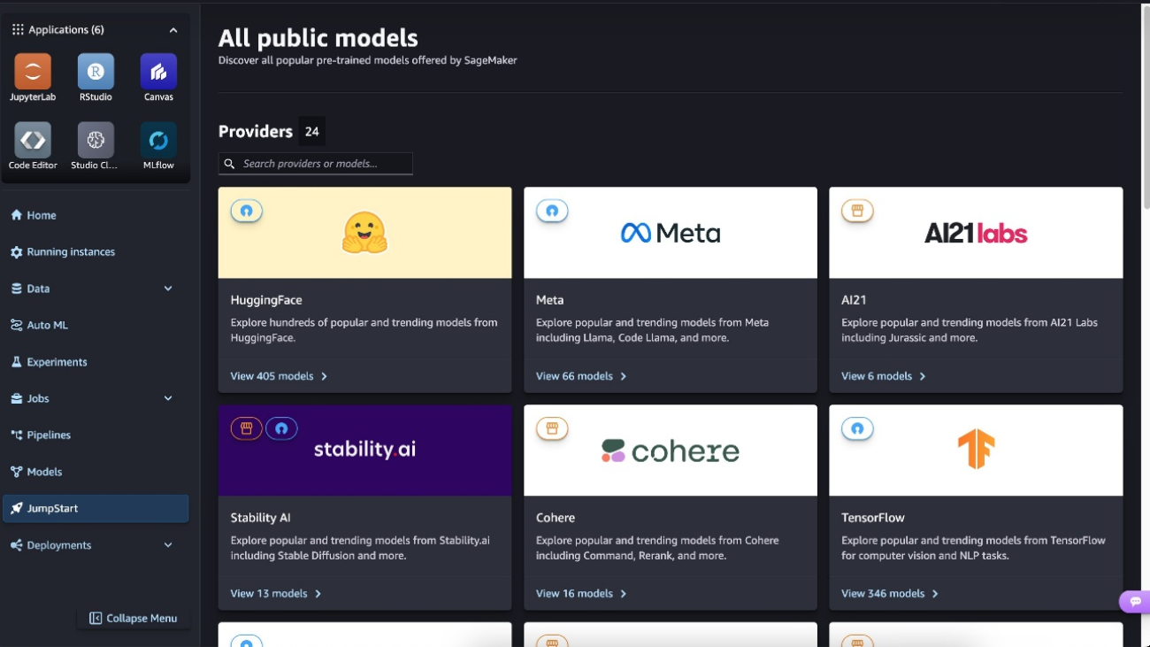


 Preston Tuggle is a Sr. Specialist Solutions Architect working on generative AI.
 Niithiyn Vijeaswaran is a GenAI Specialist Solutions Architect at AWS. His area of focus is generative AI and AWS AI Accelerators. He holds a Bachelor’s degree in Computer Science and Bioinformatics. Niithiyn works closely with the Generative AI GTM team to enable AWS customers on multiple fronts and accelerate their adoption of generative AI. He’s an avid fan of the Dallas Mavericks and enjoys collecting sneakers.
 Shane Rai is a Principal GenAI Specialist with the AWS World Wide Specialist Organization (WWSO). He works with customers across industries to solve their most pressing and innovative business needs using the breadth of cloud-based AI/ML AWS services, including model offerings from top tier foundation model providers.
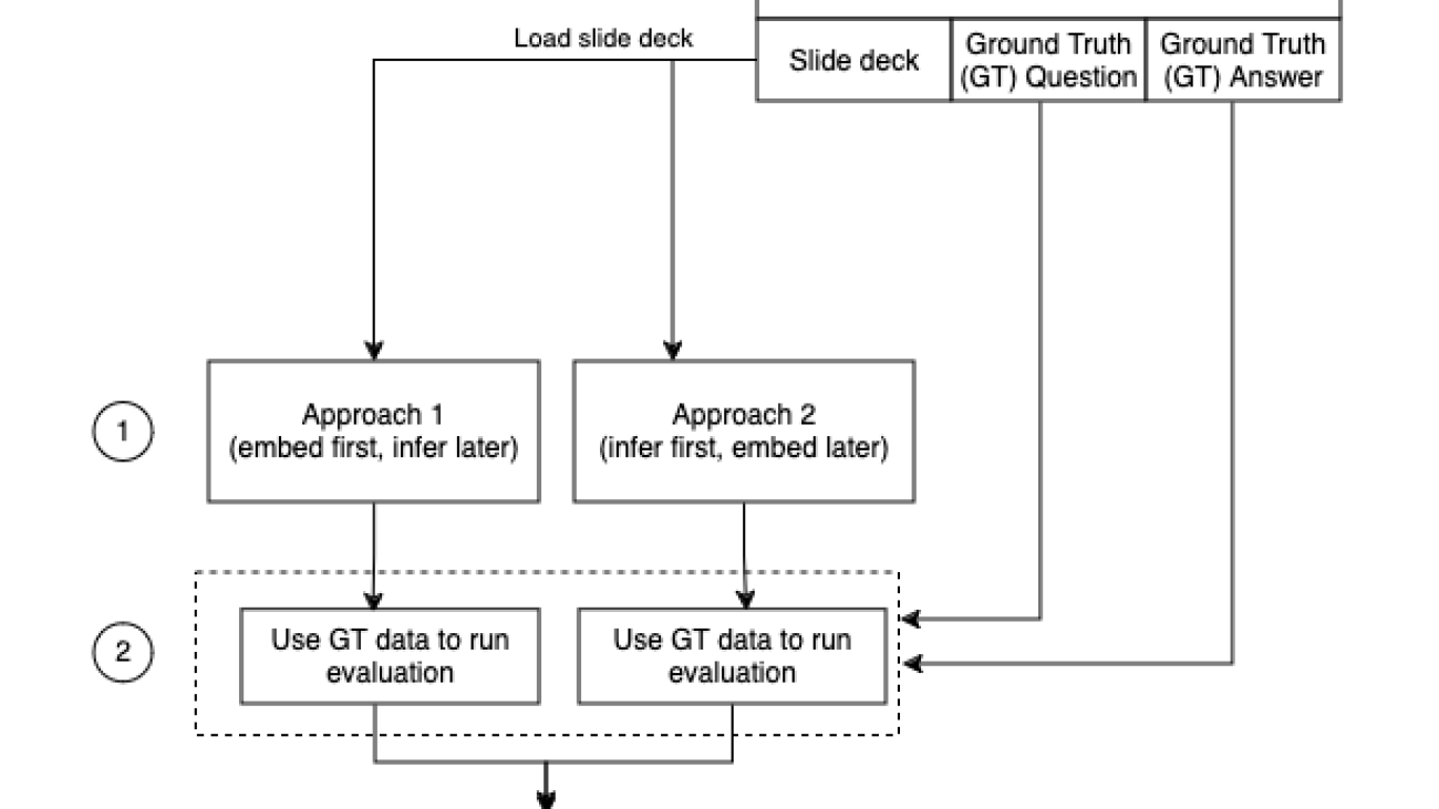

 Archana Inapudi is a Senior Solutions Architect at AWS, supporting a strategic customer. She has over a decade of cross-industry expertise leading strategic technical initiatives. Archana is an aspiring member of the AI/ML technical field community at AWS. Prior to joining AWS, Archana led a migration from traditional siloed data sources to Hadoop at a healthcare company. She is passionate about using technology to accelerate growth, provide value to customers, and achieve business outcomes.
 Manju Prasad is a Senior Solutions Architect at Amazon Web Services. She focuses on providing technical guidance in a variety of technical domains, including AI/ML. Prior to joining AWS, she designed and built solutions for companies in the financial services sector and also for a startup. She has worked in all layers of the software stack, ranging from webdev to databases, and has experience in all levels of the software development lifecycle. She is passionate about sharing knowledge and fostering interest in emerging talent.
 Amit Arora is an AI and ML Specialist Architect at Amazon Web Services, helping enterprise customers use cloud-based machine learning services to rapidly scale their innovations. He is also an adjunct lecturer in the MS data science and analytics program at Georgetown University in Washington, D.C.
 Antara Raisa is an AI and ML Solutions Architect at Amazon Web Services supporting strategic customers based out of Dallas, Texas. She also has previous experience working with large enterprise partners at AWS, where she worked as a Partner Success Solutions Architect for digital-centered customers.


 Abhishek Maligehalli Shivalingaiah is a Senior Generative AI Solutions Architect at AWS, specializing in Amazon Q Business. With a deep passion for using agentic AI frameworks to solve complex business challenges, he brings nearly a decade of expertise in developing data and AI solutions that deliver tangible value for enterprises. Beyond his professional endeavors, Abhishek is an artist who finds joy in creating portraits of family and friends, expressing his creativity through various artistic mediums.
 Marcel Pividal is a Senior AI Services Solutions Architect in the World-Wide Specialist Organization, bringing over 22 years of expertise in transforming complex business challenges into innovative technological solutions. As a thought leader in generative AI implementation, he specializes in developing secure, compliant AI architectures for enterprise-scale deployments across multiple industries.
 Sachi Sharma is a Senior Software Engineer at Amazon Q Business, specializing in generative and agentic AI. Beyond her professional pursuits, Sachi is an avid reader and coffee lover, and enjoys driving, particularly long, scenic drives.
 Manjukumar Patil is a Software Engineer at Amazon Q Business with a passion for designing and scaling AI-driven distributed systems. In his free time, he loves hiking and exploring national parks.
 James Gung is a Senior Applied Scientist at AWS whose research spans diverse topics related to conversational AI and agentive systems. Outside of work, he enjoys spending time with his family, traveling, playing violin, and bouldering.
 Najih is a Senior Software Engineer at AWS Q Business. He is passionate about designing and scaling AI based distributed systems, and excels at bringing innovative solutions to complex challenges. Outside of work, he enjoys lifting and martial arts, particularly MMA.


 Niithiyn Vijeaswaran is a Generative AI Specialist Solutions Architect with the Third-Party Model Science team at AWS. His area of focus is generative AI and AWS AI Accelerators. He holds a Bachelor’s degree in Computer Science and Bioinformatics.
 Shane Rai is a Principal Generative AI Specialist with the AWS World Wide Specialist Organization (WWSO). He works with customers across industries to solve their most pressing and innovative business needs using the breadth of cloud-based AI/ML services provided by AWS, including model offerings from top tier foundation model providers.