Companies across various scales and industries are using large language models (LLMs) to develop generative AI applications that provide innovative experiences for customers and employees. However, building or fine-tuning these pre-trained LLMs on extensive datasets demands substantial computational resources and engineering effort. With the increase in sizes of these pre-trained LLMs, the model customization process becomes complex, time-consuming, and often prohibitively expensive for most organizations that lack the necessary infrastructure and skilled talent.
In this post, we demonstrate how you can address these challenges by using fully managed environment with Amazon SageMaker Training jobs to fine-tune the Mixtral 8x7B model using PyTorch Fully Sharded Data Parallel (FSDP) and Quantized Low Rank Adaptation (QLoRA).
We guide you through a step-by-step implementation of model fine-tuning on a GEM/viggo dataset, employing the QLoRA fine-tuning strategy on a single p4d.24xlarge worker node (providing 8 Nvidia A100 40GB GPUs).
Business challenge
Today’s businesses are looking to adopt a variety of LLMs to enhance business applications. Primarily, they’re looking for foundation models (FMs) that are open source (that is, model weights that work without modification from the start) and can offer computational efficiency and versatility. Mistral’s Mixtral 8x7B model, released with open weights under the Apache 2.0 license, is one of the models that has gained popularity with large enterprises due to the high performance that it offers across various tasks. Mixtral employs a sparse mixture of experts (SMoE) architecture, selectively activating only a subset of its parameters for each input during model training. This architecture allows these models to use only 13B (about 18.5%) of its 46.7B total parameters during inference, making it high performing and efficient.
These FMs work well for many use cases but lack domain-specific information that limits their performance at certain tasks. This requires businesses to use fine-tuning strategies to adapt these large FMs to specific domains, thus improving performance on targeted applications. Due to the growing number of model parameters and the increasing context lengths of these modern LLMs, this process is memory intensive and requires advanced AI expertise to align and optimize them effectively. The cost of provisioning and managing the infrastructure increases the overall cost of ownership of the end-to-end solution.
In the upcoming section, we discuss how you can cost-effectively build such a solution with advanced memory optimization techniques using Amazon SageMaker.
Solution overview
To address the memory challenges of fine-tuning LLMs such as Mixtral, we will adopt the QLoRA method. As shown in the following diagram, QLoRA freezes the original model’s weights and adds low-rank trainable parameters to the transformer layers. QLoRA further uses quantization to represent the actual model’s weights in a compact, optimized format such as 4-bit NormalFloat (NF4), effectively compressing the model and reducing its memory footprint. This enables training and fine-tuning these LLMs even on systems with limited memory while maintaining performance comparable to half-precision fine-tuning. QLoRA’s support for double quantization and paged optimizers reduces the memory footprint further by quantizing the quantization constants and effectively handling any sudden memory demands.
During the forward pass computation of this architecture, the 4-bit weights get dequantized to bfloat16 (BF16) precision. On the other hand, the LoRA adapters continue to operate on BF16 precision data. Both (original weights and adapter output vectors) are then added together element-wise to produce the final result, denoted as h.
During the backward pass of the model, the gradients are computed with respect to only the LoRA parameters, not the original base model weights. Although the dequantized original weights are used in calculations, the original 4-bit quantized weights of the base model remain unchanged.
To adopt the following architecture, we will use the Hugging Face Parameter-Efficent Fine-tuning (PEFT) library, which integrates directly with bitsandbytes. This way, the QLoRA technique to fine-tune can be adopted with just a few lines of code.
QLoRA operates on a large FM. In the figure below, X denotes the input tokens of the training data, W is the existing model weights (quantized), and Wa, Wb are the segments of the adapters added by QLoRA. The original model’s weights (W) are frozen, and QLoRA adds adapters (Wa, Wb), which are low-rank trainable parameters, onto the existing transformer layer.
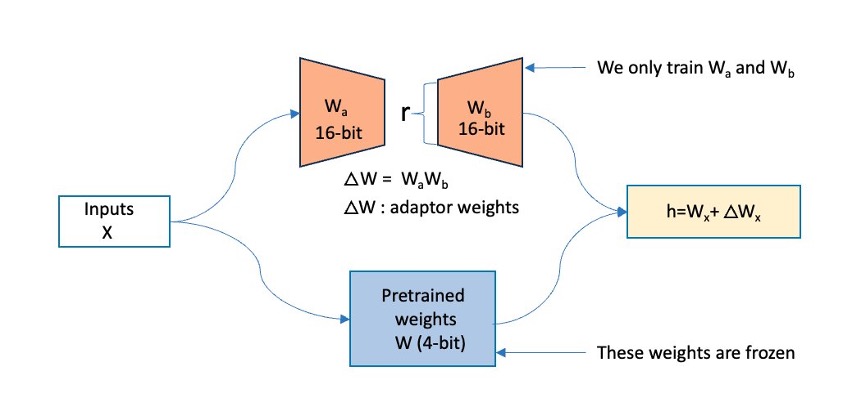
Figure 1: This figure shows how QLoRA operates. The original model’s weights (W) are frozen, and QLoRA adds in adapters (Wa, Wb) onto the existing transformer layer.
Although QLoRA helps optimize memory during fine-tuning, we will use Amazon SageMaker Training to spin up a resilient training cluster, manage orchestration, and monitor the cluster for failures. By offloading the management and maintenance of the training cluster to SageMaker, we reduce both training time and our total cost of ownership (TCO). Using this approach, you can focus on developing and refining the model while using the fully managed training infrastructure provided by SageMaker Training.
Implementation details
We spin up the cluster by calling the SageMaker control plane through APIs or the AWS Command Line Interface (AWS CLI) or using the SageMaker AWS SDK. In response, SageMaker spins up training jobs with the requested number and type of compute instances. In our example, we use one ml.p4d.24xlarge compute instance.
To take complete advantage of this multi-GPU cluster, we use the recent support of QLoRA and PyTorch FSDP. Although QLoRA reduces computational requirements and memory footprint, FSDP, a data/model parallelism technique, will help shard the model across all eight GPUs (one ml.p4d.24xlarge), enabling training the model even more efficiently. Hugging Face PEFT is where the integration happens, and you can read more about it in the PEFT documentation.
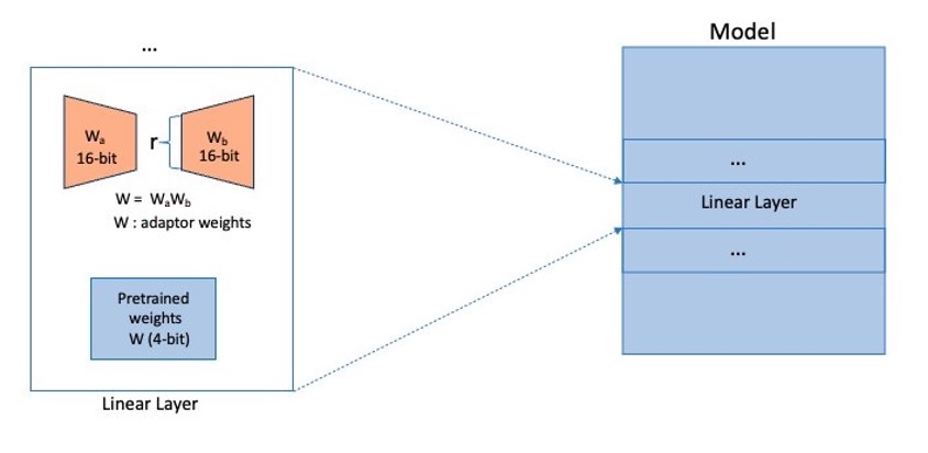
QLoRA adapters are added to the linear layers in the model. The layers (for example, transformer layers, gate networks, and feed-forward networks) put together will form the entire model, as shown in the following diagram, which will be considered to be sharded by FSDP across our cluster (shown as small shards in blue).
The following architecture diagram shows how you can use SageMaker Training to have the SageMaker Control Plane spin up a resilient training job cluster. SageMaker downloads the training image from Amazon Elastic Container Registry (Amazon ECR) and will use Amazon Simple Storage Service (Amazon S3) as an input training data source and to store training artifacts.
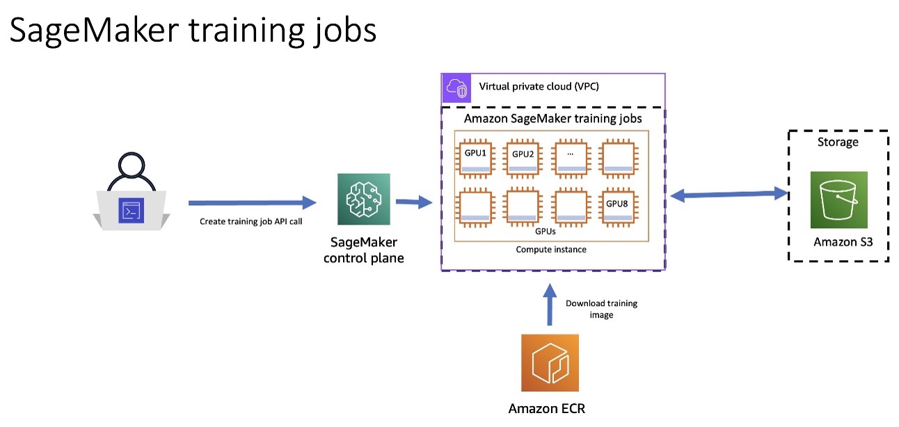
Figure 3: Architecture Diagram showing how you can utilize SageMaker Training Jobs to spin up a resilient training cluster. Amazon ECR contains the training image, and Amazon S3 contains the training artifacts.
To put this solution into practice, execute the following use case.
Prerequisites
To perform the solution, you need to have the following prerequisites in place:
- Create a Hugging Face User Access Token and get access to the gated repo mistralai/Mixtral-8x7B-v0.1 on Hugging Face.
- (Optional) Create a Weights & Biases API key to access the Weights & Biases dashboard for logging and monitoring. This is recommended if you’d like to visualize model training specific metrics.
- Request a service quota at Service Quotas for 1x
ml.p4d.24xlarge on Amazon SageMaker. To request a service quota increase, on the AWS Service Quotas console, navigate to AWS services, Amazon SageMaker, and choose ml.p4d.24xlarge for training job usage.
- Create an AWS Identity and Access Management (IAM) role with managed policies
AmazonSageMakerFullAccess and AmazonEC2FullAccess to give required access to SageMaker to run the examples.
This role is for demonstration purposes only. You need to adjust it to your specific security requirements for production. Adhere to the principle of least privilege while defining IAM policies in production.
- (Optional) Create an Amazon SageMaker Studio domain (see Quick setup to Amazon SageMaker) to access Jupyter notebooks with the preceding role. (You can use JupyterLab in your local setup too)
- Clone the GitHub repository with the assets for this deployment. This repository consists of a notebook that references training assets.
$ git clone https://github.com/aws-samples/sagemaker-distributed-training-workshop.git
$ cd 15_mixtral_finetune_qlora
The 15_mixtral_finetune_qlora directory contains the training scripts that you might need to deploy this sample.
Next, we will run the finetune-mixtral.ipynb notebook to fine-tune the Mixtral 8x7B model using QLoRA on SageMaker. Check out the notebook for more details on each step. In the next section, we walk through the key components of the fine-tuning execution.
Solution walkthrough
To perform the solution, follow the steps in the next sections.
Step 1: Set up required libraries
Install the relevant HuggingFace and SageMaker libraries:
!pip install transformers "datasets[s3]==2.18.0" "sagemaker>=2.190.0" "py7zr" "peft==0.12.0" --upgrade –quiet
Step 2: Load dataset
In this example, we use the GEM/viggo dataset from Hugging Face. This is a data-to-text generation dataset in the video game domain. The dataset is clean and organized with about 5,000 data points, and the responses are more conversational than information seeking. This type of dataset is ideal for extracting meaningful information from customer reviews. For example, an ecommerce application such as Amazon.com could use a similarly formatted dataset for fine-tuning a model for natural language processing (NLP) analysis to gauge interest in products sold. The results can be used for recommendation engines. Thus, this dataset is a good candidate for fine-tuning LLMs. To learn more about the viggo dataset, check out this research paper.
Load the dataset and convert it to the required prompt structure. The prompt is constructed with the following elements:
- Target sentence – Think of this as the final review. In the dataset, this is
target.
- Meaning representation – Think of this as a deconstructed review, broken down by attributes such as
inform, request, or give_opinion. In the dataset, this is meaning_representation.
Running the following cell gives us the train_set and test_set (training split and testing split, respectively) with structured prompts. We use the Python map function to structure the dataset splits according to our prompt.
def generate_and_tokenize_prompt(data_point):
    full_prompt = f"""
      Given a target sentence, construct the underlying
      meaning representation ...
      ['inform', 'request', 'give_opinion', 'confirm',
      'verify_attribute', 'suggest', 'request_explanation',
      'recommend', 'request_attribute']

      The attributes must be one of the following:
      ['name', 'exp_release_date', 'release_year',
      'developer', 'esrb', 'rating', 'genres',
      'player_perspective', 'has_multiplayer', 'platforms',
      'available_on_steam', 'has_linux_release',
      'has_mac_release', 'specifier']

      ### Target sentence:
      {data_point["target"]}

      ### Meaning representation:
      {data_point["meaning_representation"]}
    """
    return {"prompt": full_prompt.strip()}

# Load dataset from the HuggingFace hub
train_set = load_dataset(dataset_name, split="train")
test_set = load_dataset(dataset_name, split="test")

# Add system message to each conversation
columns_to_remove = list(dataset["train"].features)

train_dataset = train_set.map(
  generate_and_tokenize_prompt,
  remove_columns=columns_to_remove,
  batched=False
)

test_dataset = test_set.map(
  generate_and_tokenize_prompt,
  remove_columns=columns_to_remove,
  batched=False
)
Upload the dataset to Amazon S3. This step is crucial because the dataset stored in Amazon S3 will serve as the input data channel for the SageMaker training cluster. SageMaker will efficiently manage the process of distributing this data across the training cluster, allowing each node to access the necessary information for model training.
input_path = f's3://{sess.default_bucket()}/datasets/mixtral'

# Save datasets to s3
train_dataset.to_json(f"{input_path}/train/dataset.json", orient="records")
train_dataset_s3_path = f"{input_path}/train/dataset.json"
test_dataset.to_json(f"{input_path}/test/dataset.json", orient="records")
test_dataset_s3_path = f"{input_path}/test/dataset.json"
We analyze the distribution of prompt tokens to determine the maximum sequence length required for training our model in the upcoming steps.
The following graph shows the prompt tokens plotted. The x-axis is the length of the prompts, and the y-axis is the number of times that length occurs in the training dataset (frequency). We use this to determine the maximum sequence length and pad the rest of the data points accordingly. The maximum number of words in our example is 173.
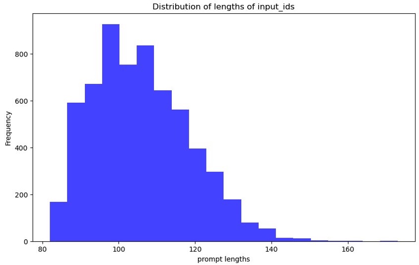
Figure 4: Graph showing the distribution of input token lengths prompted. The x-axis shows the lengths and the y-axis shows the frequency with which those input token lengths occur in the train and test dataset splits.
Step 3: Configure the parameters for SFTTrainer for the fine-tuning task
We use TrlParser to parse hyperparameters in a YAML file that is required to configure SFTTrainer API for fine-tuning the model. This approach offers flexibility because we can also overwrite the arguments specified in the config file by explicitly passing them through the command line interface.
cat > ./args.yaml <<EOF
model_id: "mistralai/Mixtral-8x7B-v0.1" # Hugging Face model id
max_seq_length: 2048 # based in prompt length distribution graph
train_dataset_path: "/opt/ml/input/data/train/" # path to where SageMaker saves train dataset
test_dataset_path: "/opt/ml/input/data/test/" # path to where SageMaker saves test dataset
output_dir: "/opt/ml/model/mixtral/adapter" # path to where SageMaker will upload the model
...

num_train_epochs: 1 # number of training epochs
per_device_train_batch_size: 10 # batch size per device during training
gradient_accumulation_steps: 1 # number of steps before performing a backward/update pass
optim: adamw_torch # use torch adamw optimizer
...

bf16: true # use bfloat16 precision
tf32: true # use tf32 precision
gradient_checkpointing: true # use gradient checkpointing to save memory

# offload FSDP parameters: https://huggingface.co/docs/transformers/main/en/fsdp
fsdp: "full_shard auto_wrap" # remove offload if enough GPU memory
fsdp_config:
  backward_prefetch: "backward_pre"
  forward_prefetch: "false"
  use_orig_params: "false"
Step 4: Review the launch script
You are now prepared to fine-tune the model using a combination of PyTorch FSDP and QLoRA. We’ve prepared a script called launch_fsdp_qlora.py that will perform the tasks mentioned in the following steps. The following is a quick review of the key points in this script before launching the training job.
- Load the dataset from a JSON file located at the specified path, using the
load_dataset function to prepare it for model training.
# Load datasets
train_dataset = load_dataset(
  "json",
  data_files=os.path.join(script_args.train_dataset_path,
  "dataset.json"),
  split="train",
)
- Prepare the tokenizer and the model.
We employ the BitsAndBytes library to configure 4-bit quantization settings for our model, enabling memory-efficient loading and computation.
By setting parameters such as load_in_4bit and bnb_4bit_use_double_quant to True, we enable a dramatic reduction in model size without significant loss in performance. The nf4 quantization type, coupled with bfloat16 compute and storage data types, allows for nuanced control over the quantization process, striking an optimal balance between model compression and accuracy preservation. This configuration enables the deployment of massive models on resource-constrained hardware, making advanced AI more accessible and practical for a wide range of applications.
# Configure model quantization
torch_dtype = torch.bfloat16
quant_storage_dtype = torch.bfloat16

# Configures 4-bit quantization settings for the model
quantization_config = BitsAndBytesConfig(
  load_in_4bit=True,
  bnb_4bit_use_double_quant=True,
  bnb_4bit_quant_type="nf4",
  bnb_4bit_compute_dtype=torch_dtype,
  bnb_4bit_quant_storage=quant_storage_dtype,
)

model_loading_params = {
  "quantization_config": quantization_config,
  "torch_dtype": quant_storage_dtype,
  "use_cache": False if
  training_args.gradient_checkpointing else True
}

# Loads a pre-trained model from the specified model ID
model = AutoModelForCausalLM.from_pretrained(
  script_args.model_id,
  cache_dir="/opt/ml/sagemaker/warmpoolcache",
  **model_loading_params
)
- Initiate the training process using SFTTrainer from the Transformer Reinforcement Learning (TRL) library to fine-tune the model. The
SFTTrainer simplifies the process of supervised fine-tuning for LLMs. This approach makes fine-tuning efficient to adapt pre-trained models to specific tasks or domains.
We use the LoraConfig class from the Hugging Face’s PEFT library to configure and add LoRA parameters (also called “adapters”) to the model.
# LoRA config based on QLoRA paper & Sebastian Raschka experiment
peft_config = LoraConfig(
  lora_alpha=8,
  lora_dropout=0.05,
  r=16,
  ...
)

################
# Training
################
trainer = SFTTrainer(
  model=model,
  args=training_args,
  train_dataset=train_dataset,
  eval_dataset=test_dataset,
  peft_config=peft_config,
  max_seq_length=script_args.max_seq_length,
  tokenizer=tokenizer,
  packing=True,
  ...
)

trainer.train(resume_from_checkpoint=checkpoint)
Step 5: Fine-tune your model
To fine-tune your model, follow the steps in the next sections.
Launch the training job
You are now ready to launch the training. We use the SageMaker Training estimator, which uses torchrun to initiate distributed training.
The SageMaker estimator simplifies the training process by automating several key tasks in this example:
- The SageMaker estimator spins up a training cluster of one
ml.p4d.24xlarge instance. SageMaker handles the setup and management of these compute instances, which reduces your TCO.
- This estimator also uses one of the pre-built containers managed by SageMaker, PyTorch, which includes an optimized compiled version of the PyTorch framework and its required dependencies and GPU-specific libraries for accelerated computations.
pytorch_estimator = PyTorch(
  entry_point= 'launch_fsdp_qlora.py',
  source_dir="./scripts",
  ...
  framework_version="2.2.0",
  py_version="py310",
  instance_count=1,
  instance_type="ml.p4d.24xlarge",
  sagemaker_session=sess,
  disable_output_compression=True,
  keep_alive_period_in_seconds=1800,
  distribution={"torch_distributed": {"enabled": True}},
  hyperparameters={
    "config": "/opt/ml/input/data/config/args.yaml" #path to
    TRL config which was uploaded to s3
  }
)
The training process generates trained adapters that will be saved in a default S3 bucket named sagemaker-<region name>-<account_id> for this job.
Monitor your training run
You can monitor training metrics, such as loss, and learning rate for your training run through the Weights & Biases Dashboard. The following figures show the results of the training run, where we track GPU utilization and GPU memory utilization.
The example is optimized to use GPU memory to its maximum capacity. Note that increasing the batch size any further will lead to CUDA Out of Memory errors.
The following graph shows the GPU memory utilization (for all eight GPUs) during the training process. You can also observe the GPU memory utilization for any given point in time.
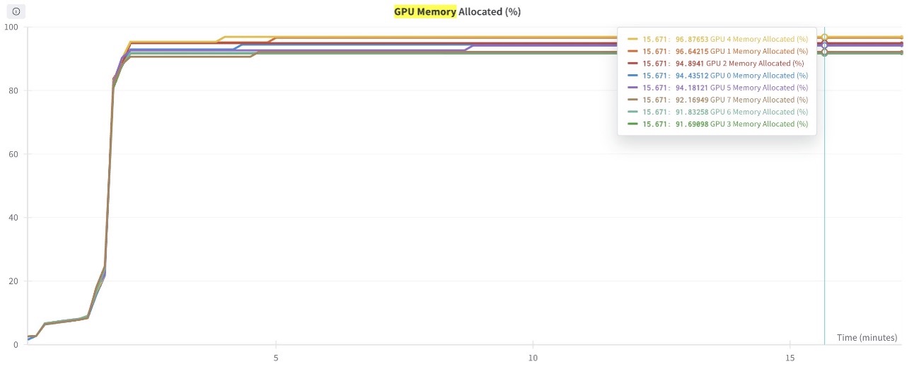
Figure 5: This graph shows the GPU Memory utilization plotted for all 8 GPUs in the training job.
The following graph shows the GPU compute utilization (for all eight GPUs) during the training process. You can also observe the GPU memory utilization for any given point in time.
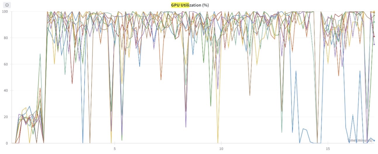
Figure 6: This graph shows the GPU Compute utilization plotted for all 8 GPUs in the training job.
Step 6: Merge the trained adapter with the base model for inference
Merge the training LoRA adapter with the base model. After the merge is complete, run inference to find the results. Specifically, look at how the new fine-tuned and merged model performs compared to the original unmodified Mixtral-8x7b model. The example does the adapter merge and inference both in the same launch script “merge_model_adapter.py.”
Before launching the training job, review the key components of the merge script:
Use the Hugging Face Transformers library. Specifically, use AutoModelForCausalLM to load a PEFT model from a specified HuggingFace model directory (mistralai/Mixtral-8x7B-v0.1). We have configured this library to have a low CPU memory utilization (low_cpu_mem_usage=True) to reduce the CPU to GPU communication overhead, and we’ve also used automatic device mapping (device_map="auto") while offloading the model to a designated folder to manage resource constraints.
# Load a Peft model
base_model = AutoModelForCausalLM.from_pretrained(
  model_id,
  low_cpu_mem_usage=True,
  #torch_dtype=torch.float16,
  device_map="auto",
  offload_folder="/opt/ml/model/"
)

# Load the adapter
peft_model = PeftModel.from_pretrained(
  base_model,
  adapter_dir,
  #torch_dtype=torch.float16,  # Set dtype to float16
  offload_folder="/opt/ml/model/"
)

# Merge the base model with the trained adapter
model = peft_model.merge_and_unload()
print("Merge done")
After the model is merged, send inference requests to generate responses.
def generate_text(model, prompt, max_length=500, num_return_sequences=1):
    ...

    input_ids = tokenizer.encode(prompt_input,
    return_tensors="pt").to(device)

    # Generate text
    with torch.no_grad():
    output = model.generate(
      input_ids,
      max_length=max_length,
      num_return_sequences=num_return_sequences,
      no_repeat_ngram_size=2,
      top_k=50,
      top_p=0.95,
      temperature=0.7
    )

    # Decode and return the generated text
    generated_texts = [tokenizer.decode(seq,
    skip_special_tokens=True) for seq in output]

    return generated_texts

print(f"nnn*** Generating Inference on Base Model: {generate_text(base_model,prompt)}nnn")

print(f"***nnn Generating Inference on Trained Model: {generate_text(model,prompt)}nnn")
Step 7: Launch the SageMaker training job to merge the adapter
Run the following script as part of the SageMaker training job.
First, explore the adapters that were saved as part of the training run.
adapter_dir_path=f"{model_artifacts}/mixtral/adapter/"

print(f'nAdapter S3 Dir path:{adapter_dir_path} n')

!aws s3 ls {adapter_dir_path}

# Reference Output
Adapter S3 Dir path:s3://sagemaker-<Region>-<Account-ID>/mixtral-8-7b-finetune-2024-09-08-22-27-42-099/output/model/mixtral/adapter/

PRE checkpoint-64/
PRE runs/
2024-09-08 23:08:07       5101 README.md
2024-09-08 23:07:58        722 adapter_config.json
2024-09-08 23:08:06  969174880 adapter_model.safetensors
2024-09-08 23:08:08        437 special_tokens_map.json
2024-09-08 23:08:04    1795596 tokenizer.json
2024-09-08 23:08:04        997 tokenizer_config.json
2024-09-08 23:08:04       5688 training_args.bin
Create and run the PyTorch estimator to configure the training job.
pytorch_estimator_adapter = PyTorch(
  entry_point= 'merge_model_adapter.py',
  source_dir="./scripts",
  job_name=job_name,
  base_job_name=job_name,
  max_run=5800,
  role=role,
  framework_version="2.2.0",
  py_version="py310",
  instance_count=1,
  instance_type="ml.p4d.24xlarge",
  sagemaker_session=sess,
  disable_output_compression=True,
  keep_alive_period_in_seconds=1800,
  hyperparameters={
    "model_id": "mistralai/Mixtral-8x7B-v0.1",  # Hugging Face model id
    "hf_token": "<hf-token>",
    "dataset_name":dataset_name
  }
)

# starting the train job with our uploaded datasets as input
pytorch_estimator_adapter.fit(data, wait=True)
Here’s the target sentence (key prompt) to generate model inference results:
Earlier, you stated that you didn't have strong feelings about PlayStation's Little Big Adventure.
Is your opinion true for all games which don't have multiplayer?
Ground truth inference (data label):
verify_attribute(name[Little Big Adventure], rating[average], has_multiplayer[no], platforms[PlayStation])
Original model inference (that is, meaning representation):
inform(name(Little Big Adventure), has_multiplayer(Little Big Adventure))
Fine-tuned model inference result (that is, meaning representation):
verify_attribute(name[Little Big Adventure], rating[average], has_multiplayer[no], platforms[PlayStation])
The preceding results compare the inference results of the fine-tuned model against both the ground truth and the inference results of the original unmodified Mixtral 8x7B model. You can observe that the fine-tuned model provides more details and better representation of the meaning than the base model. Run systematic evaluation to quantify the fine-tuned model’s improvements for your production workloads.
Clean up
To clean up your resources to avoid incurring any more charges, follow these steps:
- Delete any unused SageMaker Studio resources.
- (Optional) Delete the SageMaker Studio domain.
- Verify that your training job isn’t running anymore. To do so, on your SageMaker console, choose Training and check Training jobs.
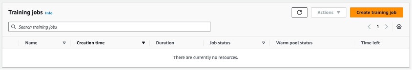
Figure 7: Screenshot showing that there are no training jobs running anymore. This is what your console should look like once you follow the clean-up steps provided
To learn more about cleaning up your provisioned resources, check out Clean up.
Conclusion
In this post, we provided you with a step-by-step guide to fine-tune the Mixtral 8x7B MoE model with QLoRA. We use SageMaker Training Jobs and the Hugging Face PEFT package for QLoRA, with bitsandbytes for quantization together to perform the fine-tuning task. The fine-tuning was conducted using the quantized model loaded on a single compute instance, which eliminates the need of a larger cluster. As observed, the model performance improved with just 50 epochs.
To learn more about Mistral on AWS and to find more examples, check out the mistral-on-aws GitHub repository. To get started, check out the notebook on the mixtral_finetune_qlora GitHub repository. To learn more about generative AI on AWS, check out Generative AI on AWS, Amazon Bedrock, and Amazon SageMaker.
About the Authors
 Aman Shanbhag is an Associate Specialist Solutions Architect on the ML Frameworks team at Amazon Web Services, where he helps customers and partners with deploying ML training and inference solutions at scale. Before joining AWS, Aman graduated from Rice University with degrees in computer science, mathematics, and entrepreneurship.
 Kanwaljit Khurmi is an AI/ML Principal Solutions Architect at Amazon Web Services. He works with AWS product teams, engineering, and customers to provide guidance and technical assistance for improving the value of their hybrid ML solutions when using AWS. Kanwaljit specializes in helping customers with containerized and machine learning applications.
 Nishant Karve is a Sr. Solutions Architect aligned with the healthcare and life sciences (HCLS) domain. He collaborates with large HCLS customers for their generative AI initiatives and guides them from ideation to production.
Read More


 Mithil Shah is a Principal AI/ML Solution Architect at Amazon Web Services. He helps commercial and public sector customers use AI/ML to achieve their business outcome. He is currently helping customers build chat bots and search functionality using LLM agents and RAG.
 Santosh Kulkarni is an Senior Solutions Architect at Amazon Web Services specializing in AI/ML. He is passionate about generative AI and is helping customers unlock business potential and drive actionable outcomes with machine learning at scale. Outside of work, he enjoys reading and traveling.


 Isaac Smothers is a Senior DevOps Engineer at Crexi. Isaac focuses on automating the creation and maintenance of robust, secure cloud infrastructure with built-in observability. Based in San Luis Obispo, he is passionate about providing self-service solutions that enable developers to build, configure, and manage their services independently, without requiring cloud or DevOps expertise. In his free time, he enjoys hiking, video editing, and gaming.
 James Healy-Mirkovich is a principal data scientist at Crexi in Los Angeles. Passionate about making data actionable and impactful, he develops and deploys customer-facing AI/ML solutions and collaborates with product teams to explore the possibilities of AI/ML. Outside work, he unwinds by playing guitar, traveling, and enjoying music and movies.
 Marina Novikova is a Senior Partner Solution Architect at AWS. Marina works on the technical co-enablement of AWS ISV Partners in the DevOps and Data and Analytics segments to enrich partner solutions and solve complex challenges for AWS customers. Outside of work, Marina spends time climbing high peaks around the world.


 Sharon Yu is a Software Development Engineer with Amazon SageMaker based in New York City.
 Saurabh Trikande is a Senior Product Manager for Amazon Bedrock and SageMaker Inference. He is passionate about working with customers and partners, motivated by the goal of democratizing AI. He focuses on core challenges related to deploying complex AI applications, inference with multi-tenant models, cost optimizations, and making the deployment of Generative AI models more accessible. In his spare time, Saurabh enjoys hiking, learning about innovative technologies, following TechCrunch, and spending time with his family.
 Michael Nguyen is a Senior Startup Solutions Architect at AWS, specializing in leveraging AI/ML to drive innovation and develop business solutions on AWS. Michael holds 12 AWS certifications and has a BS/MS in Electrical/Computer Engineering and an MBA from Penn State University, Binghamton University, and the University of Delaware.
 Dr. Xin Huang is a Senior Applied Scientist for Amazon SageMaker JumpStart and Amazon SageMaker built-in algorithms. He focuses on developing scalable machine learning algorithms. His research interests are in the area of natural language processing, explainable deep learning on tabular data, and robust analysis of non-parametric space-time clustering. He has published many papers in ACL, ICDM, KDD conferences, and Royal Statistical Society: Series A.


 Fahim Surani is a Solutions Architect at Amazon Web Services who helps customers innovate in the cloud. With a focus in Machine Learning and Generative AI, he works with global digital native companies and financial services to architect scalable, secure, and cost-effective products and services on AWS. Prior to joining AWS, he was an architect, an AI engineer, a mobile games developer, and a software engineer. In his free time he likes to run and read science fiction.
 Mark Roy is a Principal Machine Learning Architect for AWS, helping customers design and build generative AI solutions. His focus since early 2023 has been leading solution architecture efforts for the launch of Amazon Bedrock, AWS’ flagship generative AI offering for builders. Mark’s work covers a wide range of use cases, with a primary interest in generative AI, agents, and scaling ML across the enterprise. He has helped companies in insurance, financial services, media and entertainment, healthcare, utilities, and manufacturing. Prior to joining AWS, Mark was an architect, developer, and technology leader for over 25 years, including 19 years in financial services. Mark holds six AWS certifications, including the ML Specialty Certification.


 Ramesh Eega is a Global Accounts Solutions Architect based out of Atlanta, GA. He is passionate about helping customers throughout their cloud journey.


 Art Tuazon is a Solutions Architect on the CSC team at AWS. She supports both AWS Partners and customers on technical best practices. In her free time, she enjoys running and cooking.
 Beau Tse is a Partner Solutions Architect at AWS. He focuses on supporting AWS Partners through their partner journey and is passionate about enabling them on AWS. In his free time, he enjoys traveling and dancing.
 David Talby is the Chief Technology Officer at John Snow Labs, helping companies apply artificial intelligence to solve real-world problems in healthcare and life science. He was named USA CTO of the Year by the Global 100 Awards and Game Changers Awards in 2022.
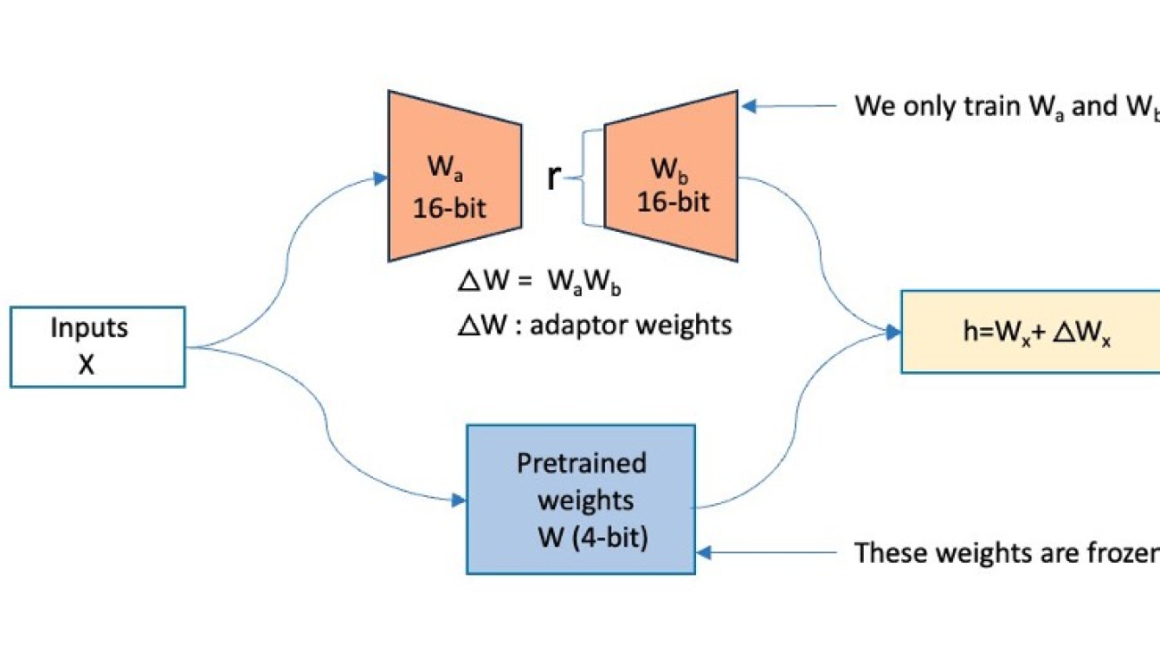


 Alan Tan is a Senior Product Manager with SageMaker, leading efforts on large model inference. He’s passionate about applying machine learning to the area of analytics. Outside of work, he enjoys the outdoors.
 Pavan Kumar Madduri is an Associate Solutions Architect at Amazon Web Services. He has a strong interest in designing innovative solutions in Generative AI and is passionate about helping customers harness the power of the cloud. He earned his MS in Information Technology from Arizona State University. Outside of work, he enjoys swimming and watching movies.