Posts in category: Amazon AWS

Natural language processing (NLP) is the field in machine learning (ML) concerned with giving computers the ability to understand text and spoken words in the same way as human beings can. Recently, state-of-the-art architectures like the transformer architecture are used to achieve near-human performance on NLP downstream tasks like text summarization, text classification, entity recognition, and more.

Large language models (LLMs) are transformer-based models trained on a large amount of unlabeled text with hundreds of millions (BERT) to over a trillion parameters (MiCS), and whose size makes single-GPU training impractical. Due to their inherent complexity, training an LLM from scratch is a very challenging task that very few organizations can afford. A common practice for NLP downstream tasks is to take a pre-trained LLM and fine-tune it. For more information about fine-tuning, refer to Domain-adaptation Fine-tuning of Foundation Models in Amazon SageMaker JumpStart on Financial data and Fine-tune transformer language models for linguistic diversity with Hugging Face on Amazon SageMaker.

Zero-shot learning in NLP allows a pre-trained LLM to generate responses to tasks that it hasn’t been explicitly trained for (even without fine-tuning). Specifically speaking about text classification, zero-shot text classification is a task in natural language processing where an NLP model is used to classify text from unseen classes, in contrast to supervised classification, where NLP models can only classify text that belong to classes in the training data.

We recently launched zero-shot classification model support in Amazon SageMaker JumpStart. SageMaker JumpStart is the ML hub of Amazon SageMaker that provides access to pre-trained foundation models (FMs), LLMs, built-in algorithms, and solution templates to help you quickly get started with ML. In this post, we show how you can perform zero-shot classification using pre-trained models in SageMaker Jumpstart. You will learn how to use the SageMaker Jumpstart UI and SageMaker Python SDK to deploy the solution and run inference using the available models.

Zero-shot learning

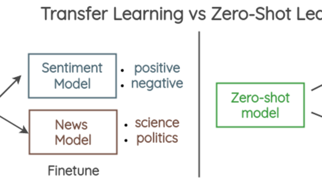
Zero-shot classification is a paradigm where a model can classify new, unseen examples that belong to classes that were not present in the training data. For example, a language model that has beed trained to understand human language can be used to classify New Year’s resolutions tweets on multiple classes like career, health, and finance, without the language model being explicitly trained on the text classification task. This is in contrast to fine-tuning the model, since the latter implies re-training the model (through transfer learning) while zero-shot learning doesn’t require additional training.

The following diagram illustrates the differences between transfer learning (left) vs. zero-shot learning (right).

Yin et al. proposed a framework for creating zero-shot classifiers using natural language inference (NLI). The framework works by posing the sequence to be classified as an NLI premise and constructs a hypothesis from each candidate label. For example, if we want to evaluate whether a sequence belongs to the class politics, we could construct a hypothesis of “This text is about politics.” The probabilities for entailment and contradiction are then converted to label probabilities. As a quick review, NLI considers two sentences: a premise and a hypothesis. The task is to determine whether the hypothesis is true (entailment) or false (contradiction) given the premise. The following table provides some examples.

Solution overview

In this post, we discuss the following:

• How to deploy pre-trained zero-shot text classification models using the SageMaker JumpStart UI and run inference on the deployed model using short text data
• How to use the SageMaker Python SDK to access the pre-trained zero-shot text classification models in SageMaker JumpStart and use the inference script to deploy the model to a SageMaker endpoint for a real-time text classification use case
• How to use the SageMaker Python SDK to access pre-trained zero-shot text classification models and use SageMaker batch transform for a batch text classification use case

SageMaker JumpStart provides one-click fine-tuning and deployment for a wide variety of pre-trained models across popular ML tasks, as well as a selection of end-to-end solutions that solve common business problems. These features remove the heavy lifting from each step of the ML process, simplifying the development of high-quality models and reducing time to deployment. The JumpStart APIs allow you to programmatically deploy and fine-tune a vast selection of pre-trained models on your own datasets.

The JumpStart model hub provides access to a large number of NLP models that enable transfer learning and fine-tuning on custom datasets. As of this writing, the JumpStart model hub contains over 300 text models across a variety of popular models, such as Stable Diffusion, Flan T5, Alexa TM, Bloom, and more.

Note that by following the steps in this section, you will deploy infrastructure to your AWS account that may incur costs.

Deploy a standalone zero-shot text classification model

In this section, we demonstrate how to deploy a zero-shot classification model using SageMaker JumpStart. You can access pre-trained models through the JumpStart landing page in Amazon SageMaker Studio. Complete the following steps:

1. In SageMaker Studio, open the JumpStart landing page.
   Refer to Open and use JumpStart for more details on how to navigate to SageMaker JumpStart.
2. In the Text Models carousel, locate the “Zero-Shot Text Classification” model card.
3. Choose View model to access the facebook-bart-large-mnli model.
   Alternatively, you can search for the zero-shot classification model in the search bar and get to the model in SageMaker JumpStart.
4. Specify a deployment configuration, SageMaker hosting instance type, endpoint name, Amazon Simple Storage Service (Amazon S3) bucket name, and other required parameters.
5. Optionally, you can specify security configurations like AWS Identity and Access Management (IAM) role, VPC settings, and AWS Key Management Service (AWS KMS) encryption keys.
6. Choose Deploy to create a SageMaker endpoint.

This step takes a couple of minutes to complete. When it’s complete, you can run inference against the SageMaker endpoint that hosts the zero-shot classification model.

In the following video, we show a walkthrough of the steps in this section.

Use JumpStart programmatically with the SageMaker SDK

In the SageMaker JumpStart section of SageMaker Studio, under Quick start solutions, you can find the solution templates. SageMaker JumpStart solution templates are one-click, end-to-end solutions for many common ML use cases. As of this writing, over 20 solutions are available for multiple use cases, such as demand forecasting, fraud detection, and personalized recommendations, to name a few.

The “Zero Shot Text Classification with Hugging Face” solution provides a way to classify text without the need to train a model for specific labels (zero-shot classification) by using a pre-trained text classifier. The default zero-shot classification model for this solution is the facebook-bart-large-mnli (BART) model. For this solution, we use the 2015 New Year’s Resolutions dataset to classify resolutions. A subset of the original dataset containing only the Resolution_Category (ground truth label) and the text columns is included in the solution’s assets.

The input data includes text strings, a list of desired categories for classification, and whether the classification is multi-label or not for synchronous (real-time) inference. For asynchronous (batch) inference, we provide a list of text strings, the list of categories for each string, and whether the classification is multi-label or not in a JSON lines formatted text file.

The result of the inference is a JSON object that looks something like the following screenshot.

We have the original text in the sequence field, the labels used for the text classification in the labels field, and the probability assigned to each label (in the same order of appearance) in the field scores.

To deploy the Zero Shot Text Classification with Hugging Face solution, complete the following steps:

1. On the SageMaker JumpStart landing page, choose Models, notebooks, solutions in the navigation pane.
2. In the Solutions section, choose Explore All Solutions.
   
3. On the Solutions page, choose the Zero Shot Text Classification with Hugging Face model card.
4. Review the deployment details and if you agree, choose Launch.
   

The deployment will provision a SageMaker real-time endpoint for real-time inference and an S3 bucket for storing the batch transformation results.

The following diagram illustrates the architecture of this method.

Perform real-time inference using a zero-shot classification model

In this section, we review how to use the Python SDK to run zero-shot text classification (using any of the available models) in real time using a SageMaker endpoint.

1. First, we configure the inference payload request to the model. This is model dependent, but for the BART model, the input is a JSON object with the following structure:

   {
   “inputs”: # The text to be classified
   “parameters”: {
   “candidate_labels”: # A list of the labels we want to use for the text classification
   “multi_label”: True | False
   }
   }

2. Note that the BART model is not explicitly trained on the candidate_labels. We will use the zero-shot classification technique to classify the text sequence to unseen classes. The following code is an example using text from the New Year’s resolutions dataset and the defined classes:

   classification_categories = ['Health', 'Humor', 'Personal Growth', 'Philanthropy', 'Leisure', 'Career', 'Finance', 'Education', 'Time Management']
   data_zero_shot = {
   "inputs": "#newyearsresolution :: read more books, no scrolling fb/checking email b4 breakfast, stay dedicated to pt/yoga to squash my achin' back!",
   "parameters": {
   "candidate_labels": classification_categories,
   "multi_label": False
   }
   }

3. Next, you can invoke a SageMaker endpoint with the zero-shot payload. The SageMaker endpoint is deployed as part of the SageMaker JumpStart solution.

   response = runtime.invoke_endpoint(EndpointName=sagemaker_endpoint_name,
   ContentType='application/json',
   Body=json.dumps(payload))
   
   parsed_response = json.loads(response['Body'].read())

4. The inference response object contains the original sequence, the labels sorted by score from max to min, and the scores per label:

   {'sequence': "#newyearsresolution :: read more books, no scrolling fb/checking email b4 breakfast, stay dedicated to pt/yoga to squash my achin' back!",
   'labels': ['Personal Growth',
   'Health',
   'Time Management',
   'Leisure',
   'Education',
   'Humor',
   'Career',
   'Philanthropy',
   'Finance'],
   'scores': [0.4198768436908722,
   0.2169460505247116,
   0.16591140627861023,
   0.09742163866758347,
   0.031757451593875885,
   0.027988269925117493,
   0.015974704176187515,
   0.015464971773326397,
   0.008658630773425102]}

Run a SageMaker batch transform job using the Python SDK

This section describes how to run batch transform inference with the zero-shot classification facebook-bart-large-mnli model using the SageMaker Python SDK. Complete the following steps:

1. Format the input data in JSON lines format and upload the file to Amazon S3.
   SageMaker batch transform will perform inference on the data points uploaded in the S3 file.
2. Set up the model deployment artifacts with the following parameters:
   1. model_id – Use huggingface-zstc-facebook-bart-large-mnli.
   2. deploy_image_uri – Use the image_uris Python SDK function to get the pre-built SageMaker Docker image for the model_id. The function returns the Amazon Elastic Container Registry (Amazon ECR) URI.
   3. deploy_source_uri – Use the script_uris utility API to retrieve the S3 URI that contains scripts to run pre-trained model inference. We specify the script_scope as inference.
   4. model_uri – Use model_uri to get the model artifacts from Amazon S3 for the specified model_id.
      

      #imports
      from sagemaker import image_uris, model_uris, script_uris, hyperparameters
      
      #set model id and version
      model_id, model_version, = (
      "huggingface-zstc-facebook-bart-large-mnli",
      "*",
      )
      
      # Retrieve the inference Docker container URI. This is the base Hugging Face container image for the default model above.
      deploy_image_uri = image_uris.retrieve(
      region=None,
      framework=None, # Automatically inferred from model_id
      image_scope="inference",
      model_id=model_id,
      model_version=model_version,
      instance_type="ml.g4dn.xlarge",
      )
      
      # Retrieve the inference script URI. This includes all dependencies and scripts for model loading, inference handling, and more.
      deploy_source_uri = script_uris.retrieve(model_id=model_id, model_version=model_version, script_scope="inference")
      
      # Retrieve the model URI. This includes the pre-trained model and parameters.
      model_uri = model_uris.retrieve(model_id=model_id, model_version=model_version, model_scope="inference") 

3. Use HF_TASK to define the task for the Hugging Face transformers pipeline and HF_MODEL_ID to define the model used to classify the text:

   # Hub model configuration <https://huggingface.co/models>
   hub = {
   'HF_MODEL_ID':'facebook/bart-large-mnli', # The model_id from the Hugging Face Hub
   'HF_TASK':'zero-shot-classification' # The NLP task that you want to use for predictions
   }

   For a complete list of tasks, see Pipelines in the Hugging Face documentation.

4. Create a Hugging Face model object to be deployed with the SageMaker batch transform job:

   # Create HuggingFaceModel class
   huggingface_model_zero_shot = HuggingFaceModel(
   model_data=model_uri, # path to your trained sagemaker model
   env=hub, # configuration for loading model from Hub
   role=role, # IAM role with permissions to create an endpoint
   transformers_version="4.17", # Transformers version used
   pytorch_version="1.10", # PyTorch version used
   py_version='py38', # Python version used
   )

5. Create a transform to run a batch job:

   # Create transformer to run a batch job
   batch_job = huggingface_model_zero_shot.transformer(
   instance_count=1,
   instance_type='ml.m5.xlarge',
   strategy='SingleRecord',
   assemble_with='Line',
   output_path=s3_path_join("s3://",sagemaker_config['S3Bucket'],"zero_shot_text_clf", "results"), # we are using the same s3 path to save the output with the input
   )

6. Start a batch transform job and use S3 data as input:

   batch_job.transform(
   data=data_upload_path,
   content_type='application/json',
   split_type='Line',
   logs=False,
   wait=True
   )

You can monitor your batch processing job on the SageMaker console (choose Batch transform jobs under Inference in the navigation pane). When the job is complete, you can check the model prediction output in the S3 file specified in output_path.

For a list of all the available pre-trained models in SageMaker JumpStart, refer to Built-in Algorithms with pre-trained Model Table. Use the keyword “zstc” (short for zero-shot text classification) in the search bar to locate all the models capable of doing zero-shot text classification.

Clean up

After you’re done running the notebook, make sure to delete all resources created in the process to ensure that the costs incurred by the assets deployed in this guide are stopped. The code to clean up the deployed resources is provided in the notebooks associated with the zero-shot text classification solution and model.

Default security configurations

The SageMaker JumpStart models are deployed using the following default security configurations:

• The models are deployed with a default SageMaker execution role. You can specify your own role or use an existing one. For more information, refer to SageMaker Roles.
• The model will not connect to a VPC and no VPC will be provisioned for your model. You can specify VPC configuration to connect to your model from within the security options. For more information, see Give SageMaker Hosted Endpoints Access to Resources in Your Amazon VPC.
• Default KMS keys will be used to encrypt your model’s artifacts. You can specify your own KMS keys or use existing one. For more information, refer to Using server-side encryption with AWS KMS keys (SSE-KMS).

To learn more about SageMaker security-related topics, check out Configure security in Amazon SageMaker.

Conclusion

In this post, we showed you how to deploy a zero-shot classification model using the SageMaker JumpStart UI and perform inference using the deployed endpoint. We used the SageMaker JumpStart New Year’s resolutions solution to show how you can use the SageMaker Python SDK to build an end-to-end solution and implement zero-shot classification application. SageMaker JumpStart provides access to hundreds of pre-trained models and solutions for tasks like computer vision, natural language processing, recommendation systems, and more. Try out the solution on your own and let us know your thoughts.

About the authors

David Laredo is a Prototyping Architect at AWS Envision Engineering in LATAM, where he has helped develop multiple machine learning prototypes. Previously, he has worked as a Machine Learning Engineer and has been doing machine learning for over 5 years. His areas of interest are NLP, time series, and end-to-end ML.

Vikram Elango is an AI/ML Specialist Solutions Architect at Amazon Web Services, based in Virginia, US. Vikram helps financial and insurance industry customers with design and thought leadership to build and deploy machine learning applications at scale. He is currently focused on natural language processing, responsible AI, inference optimization, and scaling ML across the enterprise. In his spare time, he enjoys traveling, hiking, cooking, and camping with his family.

Dr. Vivek Madan is an Applied Scientist with the Amazon SageMaker JumpStart team. He got his PhD from University of Illinois at Urbana-Champaign and was a Post Doctoral Researcher at Georgia Tech. He is an active researcher in machine learning and algorithm design and has published papers in EMNLP, ICLR, COLT, FOCS, and SODA conferences.

Read More

Amazon SageMaker is a fully managed machine learning (ML) platform that offers a comprehensive set of services that serve end-to-end ML workloads. As recommended by AWS as a best practice, customers have used separate accounts to simplify policy management for users and isolate resources by workloads and account. However, when more users and teams are using the ML platform in the cloud, monitoring the large ML workloads in a scaling multi-account environment becomes more challenging. For better observability, customers are looking for solutions to monitor the cross-account resource usage and track activities, such as job launch and running status, which is essential for their ML governance and management requirements.

SageMaker services, such as Processing, Training, and Hosting, collect metrics and logs from the running instances and push them to users’ Amazon CloudWatch accounts. To view the details of these jobs in different accounts, you need to log in to each account, find the corresponding jobs, and look into the status. There is no single pane of glass that can easily show this cross-account and multi-job information. Furthermore, the cloud admin team needs to provide individuals access to different SageMaker workload accounts, which adds additional management overhead for the cloud platform team.

In this post, we present a cross-account observability dashboard that provides a centralized view for monitoring SageMaker user activities and resources across multiple accounts. It allows the end-users and cloud management team to efficiently monitor what ML workloads are running, view the status of these workloads, and trace back different account activities at certain points of time. With this dashboard, you don’t need to navigate from the SageMaker console and click into each job to find the details of the job logs. Instead, you can easily view the running jobs and job status, troubleshoot job issues, and set up alerts when issues are identified in shared accounts, such as job failure, underutilized resources, and more. You can also control access to this centralized monitoring dashboard or share the dashboard with relevant authorities for auditing and management requirements.

Overview of solution

This solution is designed to enable centralized monitoring of SageMaker jobs and activities across a multi-account environment. The solution is designed to have no dependency on AWS Organizations, but can be adopted easily in an Organizations or AWS Control Tower environment. This solution can help the operation team have a high-level view of all SageMaker workloads spread across multiple workload accounts from a single pane of glass. It also has an option to enable CloudWatch cross-account observability across SageMaker workload accounts to provide access to monitoring telemetries such as metrics, logs, and traces from the centralized monitoring account. An example dashboard is shown in the following screenshot.

The following diagram shows the architecture of this centralized dashboard solution.

SageMaker has native integration with the Amazon EventBridge, which monitors status change events in SageMaker. EventBridge enables you to automate SageMaker and respond automatically to events such as a training job status change or endpoint status change. Events from SageMaker are delivered to EventBridge in near-real time. For more information about SageMaker events monitored by EventBridge, refer to Automating Amazon SageMaker with Amazon EventBridge. In addition to the SageMaker native events, AWS CloudTrail publishes events when you make API calls, which also streams to EventBridge so that this can be utilized by many downstream automation or monitoring use cases. In our solution, we use EventBridge rules in the workload accounts to stream SageMaker service events and API events to the monitoring account’s event bus for centralized monitoring.

In the centralized monitoring account, the events are captured by an EventBridge rule and further processed into different targets:

• A CloudWatch log group, to use for the following:
  • Auditing and archive purposes. For more information, refer to the Amazon CloudWatch Logs User Guide.
  • Analyzing log data with CloudWatch Log Insights queries. CloudWatch Logs Insights enables you to interactively search and analyze your log data in CloudWatch Logs. You can perform queries to help you more efficiently and effectively respond to operational issues. If an issue occurs, you can use CloudWatch Logs Insights to identify potential causes and validate deployed fixes.
  • Support for the CloudWatch Metrics Insights query widget for high-level operations in the CloudWatch dashboard, adding CloudWatch Insights Query to dashboards, and exporting query results.
• An AWS Lambda function to complete the following tasks:
  • Perform custom logic to augment SageMaker service events. One example is performing a metric query on the SageMaker job host’s utilization metrics when a job completion event is received.
  • Convert event information into metrics in certain log formats as ingested as EMF logs. For more information, refer to Embedding metrics within logs.

The example in this post is supported by the native CloudWatch cross-account observability feature to achieve cross-account metrics, logs, and trace access. As shown at the bottom of the architecture diagram, it integrates with this feature to enable cross-account metrics and logs. To enable this, necessary permissions and resources need to be created in both the monitoring accounts and source workload accounts.

You can use this solution for either AWS accounts managed by Organizations or standalone accounts. The following sections explain the steps for each scenario. Note that within each scenario, steps are performed in different AWS accounts. For your convenience, the account type to perform the step is highlighted at the beginning each step.

Prerequisites

Before starting this procedure, clone our source code from the GitHub repo in your local environment or AWS Cloud9. Additionally, you need the following:

• Node.js 14.15.0 (or later) and nmp installed
• The AWS Command Line Interface (AWS CLI) version 2 installed
• The AWS CDK Toolkit
• Docker Engine installed (in running state when performing the deployment procedures)

Deploy the solution in an Organizations environment

If the monitoring account and all SageMaker workload accounts are all in the same organization, the required infrastructure in the source workload accounts is created automatically via an AWS CloudFormation StackSet from the organization’s management account. Therefore, no manual infrastructure deployment into the source workload accounts is required. When a new account is created or an existing account is moved into a target organizational unit (OU), the source workload infrastructure stack will be automatically deployed and included in the scope of centralized monitoring.

Set up monitoring account resources

We need to collect the following AWS account information to set up the monitoring account resources, which we use as the inputs for the setup script later on.

To retrieve the OU path, you can go to the Organizations console, and under AWS accounts, find the information to construct the OU path. For the following example, the corresponding OU path is o-ye3wn3kyh6/r-taql/ou-taql-wu7296by/.

After you retrieve this information, run the following command to deploy the required resources on the monitoring account:

./scripts/organization-deployment/deploy-monitoring-account.sh

You can get the following outputs from the deployment. Keep a note of the outputs to use in the next step when deploying the management account stack.

Set up management account resources

We need to collect the following AWS account information to set up the management account resources, which we use as the inputs for the setup script later on.

You can deploy the management account resources by running the following command:

./scripts/organization-deployment/deploy-management-account.sh

Deploy the solution in a non-Organizations environment

If your environment doesn’t use Organizations, the monitoring account infrastructure stack is deployed in a similar manner but with a few changes. However, the workload infrastructure stack needs to be deployed manually into each workload account. Therefore, this method is suitable for an environment with a limited number of accounts. For a large environment, it’s recommended to consider using Organizations.

Set up monitoring account resources

We need to collect the following AWS account information to set up the monitoring account resources, which we use as the inputs for the setup script later on.

We can deploy the monitoring account resources by running the following command after you collect the necessary information:

./scripts/individual-deployment/deploy-monitoring-account.sh

We get the following outputs when the deployment is complete. Keep a note of the outputs to use in the next step when deploying the management account stack.

Set up workload account monitoring infrastructure

We need to collect the following AWS account information to set up the workload account monitoring infrastructure, which we use as the inputs for the setup script later on.

We can deploy the monitoring account resources by running the following command:

./scripts/individual-deployment/deploy-workload-account.sh

Visualize ML tasks on the CloudWatch dashboard

To check if the solution works, we need to run multiple SageMaker processing jobs and SageMaker training jobs on the workload accounts that we used in the previous sections. The CloudWatch dashboard is customizable based on your own scenarios. Our sample dashboard consists of widgets for visualizing SageMaker Processing jobs and SageMaker Training jobs. All jobs for monitoring workload accounts are displayed in this dashboard. In each type of job, we show three widgets, which are the total number of jobs, the number of failing jobs, and the details of each job. In our example, we have two workload accounts. Through this dashboard, we can easily find that one workload account has both processing jobs and training jobs, and another workload account only has training jobs. As with the functions we use in CloudWatch, we can set the refresh interval, specify the graph type, and zoom in or out, or we can run actions such as download logs in a CSV file.

Customize your dashboard

The solution provided in the GitHub repo includes both SageMaker Training job and SageMaker Processing job monitoring. If you want to add more dashboards to monitor other SageMaker jobs, such as batch transform jobs, you can follow the instructions in this section to customize your dashboard. By modifying the index.py file, you can customize the fields what you want to display on the dashboard. You can access all details that are captured by CloudWatch through EventBridge. In the Lambda function, you can choose the necessary fields that you want to display on the dashboard. See the following code:

@metric_scope
def lambda_handler(event, context, metrics):
    
    try:
        event_type = None
        try:
            event_type = SAGEMAKER_STAGE_CHANGE_EVENT(event["detail-type"])
        except ValueError as e:
            print("Unexpected event received")

        if event_type:
            account = event["account"]
            detail = event["detail"]

            job_detail = {
                "DashboardQuery": "True"
            }
            job_detail["Account"] = account
            job_detail["JobType"] = event_type.name

            
            metrics.set_dimensions({"account": account, "jobType": event_type.name}, use_default=False)
            metrics.set_property("JobType", event_type.value)
            
            if event_type == SAGEMAKER_STAGE_CHANGE_EVENT.PROCESSING_JOB:
                job_status = detail.get("ProcessingJobStatus")

                metrics.set_property("JobName", detail.get("ProcessingJobName"))
                metrics.set_property("ProcessingJobArn", detail.get("ProcessingJobArn"))

                job_detail["JobName"]  = detail.get("ProcessingJobName")
                job_detail["ProcessingJobArn"] = detail.get("ProcessingJobArn")
                job_detail["Status"] = job_status
                job_detail["StartTime"] = detail.get("ProcessingStartTime")
                job_detail["InstanceType"] = detail.get("ProcessingResources").get("ClusterConfig").get("InstanceType")
                job_detail["InstanceCount"] = detail.get("ProcessingResources").get("ClusterConfig").get("InstanceCount")
                if detail.get("FailureReason"):

To customize the dashboard or widgets, you can modify the source code in the monitoring-account-infra-stack.ts file. Note that the field names you use in this file should be the same as those (the keys of  job_detail) defined in the Lambda file:

 // CloudWatch Dashboard
    const sagemakerMonitoringDashboard = new cloudwatch.Dashboard(
      this, 'sagemakerMonitoringDashboard',
      {
        dashboardName: Parameters.DASHBOARD_NAME,
        widgets: []
      }
    )

    // Processing Job
    const processingJobCountWidget = new cloudwatch.GraphWidget({
      title: "Total Processing Job Count",
      stacked: false,
      width: 12,
      height: 6,
      left:[
        new cloudwatch.MathExpression({
          expression: `SEARCH('{${AWS_EMF_NAMESPACE},account,jobType} jobType="PROCESSING_JOB" MetricName="ProcessingJobCount_Total"', 'Sum', 300)`,
          searchRegion: this.region,
          label: "${PROP('Dim.account')}",
        })
      ]
    });
    processingJobCountWidget.position(0,0)
    const processingJobFailedWidget = new cloudwatch.GraphWidget({
      title: "Failed Processing Job Count",
      stacked: false,
      width: 12,
      height:6,
      right:[
        new cloudwatch.MathExpression({
          expression: `SEARCH('{${AWS_EMF_NAMESPACE},account,jobType} jobType="PROCESSING_JOB" MetricName="ProcessingJobCount_Failed"', 'Sum', 300)`,
          searchRegion: this.region,
          label: "${PROP('Dim.account')}",
        })
      ]
    })
    processingJobFailedWidget.position(12,0)
    
    const processingJobInsightsQueryWidget = new cloudwatch.LogQueryWidget(
      {
        title: 'SageMaker Processing Job History',
        logGroupNames: [ingesterLambda.logGroup.logGroupName],
        view: cloudwatch.LogQueryVisualizationType.TABLE,
        queryLines: [
          'sort @timestamp desc',
          'filter DashboardQuery == "True"',
          'filter JobType == "PROCESSING_JOB"',
          'fields Account, JobName, Status, Duration, InstanceCount, InstanceType, Host, fromMillis(StartTime) as StartTime, FailureReason',
          'fields Metrics.CPUUtilization as CPUUtil, Metrics.DiskUtilization as DiskUtil, Metrics.MemoryUtilization as MemoryUtil',
          'fields Metrics.GPUMemoryUtilization as GPUMemoeyUtil, Metrics.GPUUtilization as GPUUtil',
        ],
        width:24,
        height: 6,
      }
    );
    processingJobInsightsQueryWidget.position(0, 6)
    sagemakerMonitoringDashboard.addWidgets(processingJobCountWidget);
    sagemakerMonitoringDashboard.addWidgets(processingJobFailedWidget);
    sagemakerMonitoringDashboard.addWidgets(processingJobInsightsQueryWidget);

After you modify the dashboard, you need to redeploy this solution from scratch. You can run the Jupyter notebook provided in the GitHub repo to rerun the SageMaker pipeline, which will launch the SageMaker Processing jobs again. When the jobs are finished, you can go to the CloudWatch console, and under Dashboards in the navigation pane, choose Custom Dashboards. You can find the dashboard named SageMaker-Monitoring-Dashboard.

Clean up

If you no longer need this custom dashboard, you can clean up the resources. To delete all the resources created, use the code in this section. The cleanup is slightly different for an Organizations environment vs. a non-Organizations environment.

For an Organizations environment, use the following code:

make destroy-management-stackset # Execute against the management account
make destroy-monitoring-account-infra # Execute against the monitoring account

For a non-Organizations environment, use the following code:

make destroy-workload-account-infra # Execute against each workload account
make destroy-monitoring-account-infra # Execute against the monitoring account

Alternatively, you can log in to the monitoring account, workload account, and management account to delete the stacks from the CloudFormation console.

Conclusion

In this post, we discussed the implementation of a centralized monitoring and reporting solution for SageMaker using CloudWatch. By following the step-by-step instructions outlined in this post, you can create a multi-account monitoring dashboard that displays key metrics and consolidates logs related to their various SageMaker jobs from different accounts in real time. With this centralized monitoring dashboard, you can have better visibility into the activities of SageMaker jobs across multiple accounts, troubleshoot issues more quickly, and make informed decisions based on real-time data. Overall, the implementation of a centralized monitoring and reporting solution using CloudWatch offers an efficient way for organizations to manage their cloud-based ML infrastructure and resource utilization.

Please try out the solution and send us the feedback, either in the AWS forum for Amazon SageMaker, or through your usual AWS contacts.

To learn more about the cross-account observability feature, please refer to the blog Amazon CloudWatch Cross-Account Observability

About the Authors

Jie Dong is an AWS Cloud Architect based in Sydney, Australia. Jie is passionate about automation, and loves to develop solutions to help customer improve productivity. Event-driven system and serverless framework are his expertise. In his own time, Jie loves to work on building smart home and explore new smart home gadgets.

Melanie Li, PhD, is a Senior AI/ML Specialist TAM at AWS based in Sydney, Australia. She helps enterprise customers build solutions using state-of-the-art AI/ML tools on AWS and provides guidance on architecting and implementing ML solutions with best practices. In her spare time, she loves to explore nature and spend time with family and friends.

Gordon Wang, is a Senior AI/ML Specialist TAM at AWS. He supports strategic customers with AI/ML best practices cross many industries. He is passionate about computer vision, NLP, Generative AI and MLOps. In his spare time, he loves running and hiking.

Read More

Creative advertising has the potential to be revolutionized by generative AI (GenAI). You can now create a wide variation of novel images, such as product shots, by retraining a GenAI model and providing a few inputs into the model, such as textual prompts (sentences describing the scene and objects to be produced by the model). This technique has shown promising results starting in 2022 with the explosion of a new class of foundation models (FMs) called latent diffusion models such as Stable Diffusion, Midjourney, and Dall-E-2. However, to use these models in production, the generation process requires constant refining to generate consistent outputs. This often means creating a large number of sample images of the product and clever prompt engineering, which makes the task difficult at scale.

In this post, we explore how this transformative technology can be harnessed to generate captivating and innovative advertisements at scale, especially when dealing with large catalogs of images. By using the power of GenAI, specifically through the technique of inpainting, we can seamlessly create image backgrounds, resulting in visually stunning and engaging content and reducing unwanted image artifacts (termed model hallucinations). We also delve into the practical implementation of this technique by utilizing Amazon SageMaker endpoints, which enable efficient deployment of the GenAI models driving this creative process.

We use inpainting as the key technique within GenAI-based image generation because it offers a powerful solution for replacing missing elements in images. However, this presents certain challenges. For instance, precise control over the positioning of objects within the image can be limited, leading to potential issues such as image artifacts, floating objects, or unblended boundaries, as shown in the following example images.

To overcome this, we propose in this post to strike a balance between creative freedom and efficient production by generating a multitude of realistic images using minimal supervision. To scale the proposed solution for production and streamline the deployment of AI models in the AWS environment, we demonstrate it using SageMaker endpoints.

In particular, we propose to split the inpainting process as a set of layers, each one potentially with a different set of prompts. The process can be summarized as the following steps:

1. First, we prompt for a general scene (for example, “park with trees in the back”) and randomly place the object on that background.
2. Next, we add a layer in the lower mid-section of the object by prompting where the object lies (for example, “picnic on grass, or wooden table”).
3. Finally, we add a layer similar to the background layer on the upper mid-section of the object using the same prompt as the background.

The benefit of this process is the improvement in the realism of the object because it’s perceived with better scaling and positioning relative to the background environment that matches with human expectations. The following figure shows the steps of the proposed solution.

Solution overview

To accomplish the tasks, the following flow of the data is considered:

1. Segment Anything Model (SAM) and Stable Diffusion Inpainting models are hosted in SageMaker endpoints.
2. A background prompt is used to create a generated background image using the Stable Diffusion model
3. A base product image is passed through SAM to generate a mask. The inverse of the mask is called the anti-mask.
4. The generated background image, mask, along with foreground prompts and negative prompts are used as input to the Stable Diffusion Inpainting model to generate a generated intermediate background image.
5. Similarly, the generated background image, anti-mask, along with foreground prompts and negative prompts are used as input to the Stable Diffusion Inpainting model to generate a generated intermediate foreground image.
6. The final output of the generated product image is obtained by combining the generated intermediate foreground image and generated intermediate background image.

Prerequisites

We have developed an AWS CloudFormation template that will create the SageMaker notebooks used to deploy the endpoints and run inference.

You will need an AWS account with AWS Identity and Access Management (IAM) roles that provides access to the following:

• AWS CloudFormation
• SageMaker
  • Although SageMaker endpoints provide instances to run ML models, in order to run heavy workloads like generative AI models, we use the GPU-enabled SageMaker endpoints. Refer to Amazon SageMaker Pricing for more information about pricing.
  • We use the NVIDIA A10G-enabled instance ml.g5.2xlarge to host the models.
• Amazon Simple Storage Service (Amazon S3)

For more details, check out the GitHub repository and the CloudFormation template.

Mask the area of interest of the product

In general, we need to provide an image of the object that we want to place and a mask delineating the contour of the object. This can be done using tools such as Amazon SageMaker Ground Truth. Alternatively, we can automatically segment the object using AI tools such as Segment Anything Models (SAM), assuming that the object is in the center of the image.

Use SAM to generate a mask

With SAM, an advanced generative AI technique, we can effortlessly generate high-quality masks for various objects within images. SAM uses deep learning models trained on extensive datasets to accurately identify and segment objects of interest, providing precise boundaries and pixel-level masks. This breakthrough technology revolutionizes image processing workflows by automating the time-consuming and labor-intensive task of manually creating masks. With SAM, businesses and individuals can now rapidly generate masks for object recognition, image editing, computer vision tasks, and more, unlocking a world of possibilities for visual analysis and manipulation.

Host the SAM model on a SageMaker endpoint

We use the notebook 1_HostGenAIModels.ipynb to create SageMaker endpoints and host the SAM model.

We use the inference code in inference_sam.py and package that into a code.tar.gz file, which we use to create the SageMaker endpoint. The code downloads the SAM model, hosts it on an endpoint, and provides an entry point to run inference and generate output:

SAM_ENDPOINT_NAME = 'sam-pytorch-' + str(datetime.utcnow().strftime('%Y-%m-%d-%H-%M-%S-%f'))
prefix_sam = "SAM/demo-custom-endpoint"
model_data_sam = s3.S3Uploader.upload("code.tar.gz", f's3://{bucket}/{prefix_sam}')
model_sam = PyTorchModel(entry_point='inference_sam.py',
                         model_data=model_data_sam,
                         framework_version='1.12',
                         py_version='py38',  
                         role=role,
                         env={'TS_MAX_RESPONSE_SIZE':'2000000000', 'SAGEMAKER_MODEL_SERVER_TIMEOUT' : '300'},
                         sagemaker_session=sess,      
                         name='model-'+SAM_ENDPOINT_NAME)
predictor_sam = model_sam.deploy(initial_instance_count=1,
                                 instance_type=INSTANCE_TYPE,
                                 deserializers=JSONDeserializer(),
                                 endpoint_name=SAM_ENDPOINT_NAME)

Invoke the SAM model and generate a mask

The following code is part of the 2_GenerateInPaintingImages.ipynb notebook, which is used to run the endpoints and generate results:

raw_image = Image.open("images/speaker.png").convert("RGB")
predictor_sam = PyTorchPredictor(endpoint_name=SAM_ENDPOINT_NAME,
                                 deserializer=JSONDeserializer())
output_array = predictor_sam.predict(raw_image, initial_args={'Accept': 'application/json'})
mask_image = Image.fromarray(np.array(output_array).astype(np.uint8))
# save the mask image using PIL Image
mask_image.save('images/speaker_mask.png')

The following figure shows the resulting mask obtained from the product image.

Use inpainting to create a generated image

By combining the power of inpainting with the mask generated by SAM and the user’s prompt, we can create remarkable generated images. Inpainting utilizes advanced generative AI techniques to intelligently fill in the missing or masked regions of an image, seamlessly blending them with the surrounding content. With the SAM-generated mask as guidance and the user’s prompt as a creative input, inpainting algorithms can generate visually coherent and contextually appropriate content, resulting in stunning and personalized images. This fusion of technologies opens up endless creative possibilities, allowing users to transform their visions into vivid, captivating visual narratives.

Host a Stable Diffusion Inpainting model on a SageMaker endpoint

Similarly to 2.1, we use the notebook 1_HostGenAIModels.ipynb to create SageMaker endpoints and host the Stable Diffusion Inpainting model.

We use the inference code in inference_inpainting.py and package that into a code.tar.gz file, which we use to create the SageMaker endpoint. The code downloads the Stable Diffusion Inpainting model, hosts it on an endpoint, and provides an entry point to run inference and generate output:

INPAINTING_ENDPOINT_NAME = 'inpainting-pytorch-' + str(datetime.utcnow().strftime('%Y-%m-%d-%H-%M-%S-%f'))
prefix_inpainting = "InPainting/demo-custom-endpoint"
model_data_inpainting = s3.S3Uploader.upload("code.tar.gz", f"s3://{bucket}/{prefix_inpainting}")

model_inpainting = PyTorchModel(entry_point='inference_inpainting.py',
                                model_data=model_data_inpainting,       
                                framework_version='1.12',
                                py_version='py38',
                                role=role,
                                env={'TS_MAX_RESPONSE_SIZE':'2000000000', 'SAGEMAKER_MODEL_SERVER_TIMEOUT' : '300'},
                                sagemaker_session=sess,
                                name='model-'+INPAINTING_ENDPOINT_NAME)

predictor_inpainting = model_inpainting.deploy(initial_instance_count=1,
                                               instance_type=INSTANCE_TYPE,
                                               serializer=JSONSerializer(),
                                               deserializers=JSONDeserializer(),
                                               endpoint_name=INPAINTING_ENDPOINT_NAME,
                                               volume_size=128)

Invoke the Stable Diffusion Inpainting model and generate a new image

Similarly to the step to invoke the SAM model, the notebook 2_GenerateInPaintingImages.ipynb is used to run the inference on the endpoints and generate results:

raw_image = Image.open("images/speaker.png").convert("RGB")
mask_image = Image.open('images/speaker_mask.png').convert('RGB')
prompt_fr = "table and chair with books"
prompt_bg = "window and couch, table"
negative_prompt = "longbody, lowres, bad anatomy, bad hands, missing fingers, extra digit, fewer digits, cropped, worst quality, low quality, letters"

inputs = {}
inputs["image"] = np.array(raw_image)
inputs["mask"] = np.array(mask_image)
inputs["prompt_fr"] = prompt_fr
inputs["prompt_bg"] = prompt_bg
inputs["negative_prompt"] = negative_prompt

predictor_inpainting = PyTorchPredictor(endpoint_name=INPAINTING_ENDPOINT_NAME,
                                        serializer=JSONSerializer(),
                                        deserializer=JSONDeserializer())

output_array = predictor_inpainting.predict(inputs, initial_args={'Accept': 'application/json'})
gai_image = Image.fromarray(np.array(output_array[0]).astype(np.uint8))
gai_background = Image.fromarray(np.array(output_array[1]).astype(np.uint8))
gai_mask = Image.fromarray(np.array(output_array[2]).astype(np.uint8))
post_image = Image.fromarray(np.array(output_array[3]).astype(np.uint8))

# save the generated image using PIL Image
post_image.save('images/speaker_generated.png')

The following figure shows the refined mask, generated background, generated product image, and postprocessed image.

The generated product image uses the following prompts:

• Background generation – “chair, couch, window, indoor”
• Inpainting – “besides books”

Clean up

In this post, we use two GPU-enabled SageMaker endpoints, which contributes to the majority of the cost. These endpoints should be turned off to avoid extra cost when the endpoints are not being used. We have provided a notebook, 3_CleanUp.ipynb, which can assist in cleaning up the endpoints. We also use a SageMaker notebook to host the models and run inference. Therefore, it’s good practice to stop the notebook instance if it’s not being used.

Conclusion

Generative AI models are generally large-scale ML models that require specific resources to run efficiently. In this post, we demonstrated, using an advertising use case, how SageMaker endpoints offer a scalable and managed environment for hosting generative AI models such as the text-to-image foundation model Stable Diffusion. We demonstrated how two models can be hosted and run as needed, and multiple models can also be hosted from a single endpoint. This eliminates the complexities associated with infrastructure provisioning, scalability, and monitoring, enabling organizations to focus solely on deploying their models and serving predictions to solve their business challenges. With SageMaker endpoints, organizations can efficiently deploy and manage multiple models within a unified infrastructure, achieving optimal resource utilization and reducing operational overhead.

The detailed code is available on GitHub. The code demonstrates the use of AWS CloudFormation and the AWS Cloud Development Kit (AWS CDK) to automate the process of creating SageMaker notebooks and other required resources.

About the authors

Fabian Benitez-Quiroz is a IoT Edge Data Scientist in AWS Professional Services. He holds a PhD in Computer Vision and Pattern Recognition from The Ohio State University. Fabian is involved in helping customers run their machine learning models with low latency on IoT devices and in the cloud across various industries.

Romil Shah is a Sr. Data Scientist at AWS Professional Services. Romil has more than 6 years of industry experience in computer vision, machine learning, and IoT edge devices. He is involved in helping customers optimize and deploy their machine learning models for edge devices and on the cloud. He works with customers to create strategies for optimizing and deploying foundation models.

Han Man is a Senior Data Science & Machine Learning Manager with AWS Professional Services based in San Diego, CA. He has a PhD in Engineering from Northwestern University and has several years of experience as a management consultant advising clients in manufacturing, financial services, and energy. Today, he is passionately working with key customers from a variety of industry verticals to develop and implement ML and GenAI solutions on AWS.

Read More

Amazon SageMaker offers several ways to run distributed data processing jobs with Apache Spark, a popular distributed computing framework for big data processing.

You can run Spark applications interactively from Amazon SageMaker Studio by connecting SageMaker Studio notebooks and AWS Glue Interactive Sessions to run Spark jobs with a serverless cluster. With interactive sessions, you can choose Apache Spark or Ray to easily process large datasets, without worrying about cluster management.

Alternately, if you need more control over the environment, you can use a pre-built SageMaker Spark container to run Spark applications as batch jobs on a fully managed distributed cluster with Amazon SageMaker Processing. This option allows you to select several types of instances (compute optimized, memory optimized, and more), the number of nodes in the cluster, and the cluster configuration, thereby enabling greater flexibility for data processing and model training.

Finally, you can run Spark applications by connecting Studio notebooks with Amazon EMR clusters, or by running your Spark cluster on Amazon Elastic Compute Cloud (Amazon EC2).

All these options allow you to generate and store Spark event logs to analyze them through the web-based user interface commonly named the Spark UI, which runs a Spark History Server to monitor the progress of Spark applications, track resource usage, and debug errors.

In this post, we share a solution for installing and running Spark History Server on SageMaker Studio and accessing the Spark UI directly from the SageMaker Studio IDE, for analyzing Spark logs produced by different AWS services (AWS Glue Interactive Sessions, SageMaker Processing jobs, and Amazon EMR) and stored in an Amazon Simple Storage Service (Amazon S3) bucket.

Solution overview

The solution integrates Spark History Server into the Jupyter Server app in SageMaker Studio. This allows users to access Spark logs directly from the SageMaker Studio IDE. The integrated Spark History Server supports the following:

• Accessing logs generated by SageMaker Processing Spark jobs
• Accessing logs generated by AWS Glue Spark applications
• Accessing logs generated by self-managed Spark clusters and Amazon EMR

A utility command line interface (CLI) called sm-spark-cli is also provided for interacting with the Spark UI from the SageMaker Studio system terminal. The sm-spark-cli enables managing Spark History Server without leaving SageMaker Studio.

The solution consists of shell scripts that perform the following actions:

• Install Spark on the Jupyter Server for SageMaker Studio user profiles or for a SageMaker Studio shared space
• Install the sm-spark-cli for a user profile or shared space

Install the Spark UI manually in a SageMaker Studio domain

To host Spark UI on SageMaker Studio, complete the following steps:

1. Choose System terminal from the SageMaker Studio launcher.

2. Run the following commands in the system terminal:

curl -LO https://github.com/aws-samples/amazon-sagemaker-spark-ui/releases/download/v0.1.0/amazon-sagemaker-spark-ui-0.1.0.tar.gz
tar -xvzf amazon-sagemaker-spark-ui-0.1.0.tar.gz

cd amazon-sagemaker-spark-ui-0.1.0/install-scripts
chmod +x install-history-server.sh
./install-history-server.sh

The commands will take a few seconds to complete.

3. When the installation is complete, you can start the Spark UI by using the provided sm-spark-cli and access it from a web browser by running the following code:

sm-spark-cli start s3://DOC-EXAMPLE-BUCKET/<SPARK_EVENT_LOGS_LOCATION>

The S3 location where the event logs produced by SageMaker Processing, AWS Glue, or Amazon EMR are stored can be configured when running Spark applications.

For SageMaker Studio notebooks and AWS Glue Interactive Sessions, you can set up the Spark event log location directly from the notebook by using the sparkmagic kernel.

The sparkmagic kernel contains a set of tools for interacting with remote Spark clusters through notebooks. It offers magic (%spark, %sql) commands to run Spark code, perform SQL queries, and configure Spark settings like executor memory and cores.

For the SageMaker Processing job, you can configure the Spark event log location directly from the SageMaker Python SDK.

Refer to the AWS documentation for additional information:

• For SageMaker Processing, refer to PySparkProcessor
• For AWS Glue Interactive Sessions, refer to Configuring the Spark UI (console)
• For Amazon EMR, refer to Configure an output location

You can choose the generated URL to access the Spark UI.

The following screenshot shows an example of the Spark UI.

You can check the status of the Spark History Server by using the sm-spark-cli status command in the Studio System terminal.

You can also stop the Spark History Server when needed.

Automate the Spark UI installation for users in a SageMaker Studio domain

As an IT admin, you can automate the installation for SageMaker Studio users by using a lifecycle configuration. This can be done for all user profiles under a SageMaker Studio domain or for specific ones. See Customize Amazon SageMaker Studio using Lifecycle Configurations for more details.

You can create a lifecycle configuration from the install-history-server.sh script and attach it to an existing SageMaker Studio domain. The installation is run for all the user profiles in the domain.

From a terminal configured with the AWS Command Line Interface (AWS CLI) and appropriate permissions, run the following commands:

curl -LO https://github.com/aws-samples/amazon-sagemaker-spark-ui/releases/download/v0.1.0/amazon-sagemaker-spark-ui-0.1.0.tar.gz
tar -xvzf amazon-sagemaker-spark-ui-0.1.0.tar.gz

cd amazon-sagemaker-spark-ui-0.1.0/install-scripts

LCC_CONTENT=`openssl base64 -A -in install-history-server.sh`

aws sagemaker create-studio-lifecycle-config 
	--studio-lifecycle-config-name install-spark-ui-on-jupyterserver 
	--studio-lifecycle-config-content $LCC_CONTENT 
	--studio-lifecycle-config-app-type JupyterServer 
	--query 'StudioLifecycleConfigArn'

aws sagemaker update-domain 
	--region {YOUR_AWS_REGION} 
	--domain-id {YOUR_STUDIO_DOMAIN_ID} 
	--default-user-settings 
	'{
	"JupyterServerAppSettings": {
	"DefaultResourceSpec": {
	"LifecycleConfigArn": "arn:aws:sagemaker:{YOUR_AWS_REGION}:{YOUR_STUDIO_DOMAIN_ID}:studio-lifecycle-config/install-spark-ui-on-jupyterserver",
	"InstanceType": "system"
	},
	"LifecycleConfigArns": [
	"arn:aws:sagemaker:{YOUR_AWS_REGION}:{YOUR_STUDIO_DOMAIN_ID}:studio-lifecycle-config/install-spark-ui-on-jupyterserver"
	]
	}}'

After Jupyter Server restarts, the Spark UI and the sm-spark-cli will be available in your SageMaker Studio environment.

Clean up

In this section, we show you how to clean up the Spark UI in a SageMaker Studio domain, either manually or automatically.

Manually uninstall the Spark UI

To manually uninstall the Spark UI in SageMaker Studio, complete the following steps:

1. Choose System terminal in the SageMaker Studio launcher.

2. Run the following commands in the system terminal:

cd amazon-sagemaker-spark-ui-0.1.0/install-scripts

chmod +x uninstall-history-server.sh
./uninstall-history-server.sh

Uninstall the Spark UI automatically for all SageMaker Studio user profiles

To automatically uninstall the Spark UI in SageMaker Studio for all user profiles, complete the following steps:

1. On the SageMaker console, choose Domains in the navigation pane, then choose the SageMaker Studio domain.

2. On the domain details page, navigate to the Environment tab.
3. Select the lifecycle configuration for the Spark UI on SageMaker Studio.
4. Choose Detach.

5. Delete and restart the Jupyter Server apps for the SageMaker Studio user profiles.

Conclusion

In this post, we shared a solution you can use to quickly install the Spark UI on SageMaker Studio. With the Spark UI hosted on SageMaker, machine learning (ML) and data engineering teams can use scalable cloud compute to access and analyze Spark logs from anywhere and speed up their project delivery. IT admins can standardize and expedite the provisioning of the solution in the cloud and avoid proliferation of custom development environments for ML projects.

All the code shown as part of this post is available in the GitHub repository.

About the Authors

Giuseppe Angelo Porcelli is a Principal Machine Learning Specialist Solutions Architect for Amazon Web Services. With several years software engineering and an ML background, he works with customers of any size to understand their business and technical needs and design AI and ML solutions that make the best use of the AWS Cloud and the Amazon Machine Learning stack. He has worked on projects in different domains, including MLOps, computer vision, and NLP, involving a broad set of AWS services. In his free time, Giuseppe enjoys playing football.

Bruno Pistone is an AI/ML Specialist Solutions Architect for AWS based in Milan. He works with customers of any size, helping them understand their technical needs and design AI and ML solutions that make the best use of the AWS Cloud and the Amazon Machine Learning stack. His field of expertice includes machine learning end to end, machine learning endustrialization, and generative AI. He enjoys spending time with his friends and exploring new places, as well as traveling to new destinations.

Read More

Artificial intelligence (AI) adoption is accelerating across industries and use cases. Recent scientific breakthroughs in deep learning (DL), large language models (LLMs), and generative AI is allowing customers to use advanced state-of-the-art solutions with almost human-like performance. These complex models often require hardware acceleration because it enables not only faster training but also faster inference when using deep neural networks in real-time applications. GPUs’ large number of parallel processing cores makes them well-suited for these DL tasks.

However, in addition to model invocation, those DL application often entail preprocessing or postprocessing in an inference pipeline. For example, input images for an object detection use case might need to be resized or cropped before being served to a computer vision model, or tokenization of text inputs before being used in an LLM. NVIDIA Triton is an open-source inference server that enables users to define such inference pipelines as an ensemble of models in the form of a Directed Acyclic Graph (DAG). It is designed to run models at scale on both CPU and GPU. Amazon SageMaker supports deploying Triton seamlessly, allowing you to use Triton’s features while also benefiting from SageMaker capabilities: a managed, secured environment with MLOps tools integration, automatic scaling of hosted models, and more.

AWS, in its dedication to help customers achieve the highest saving, has continuously innovated not only in pricing options and cost-optimization proactive services, but also in launching cost savings features like multi-model endpoints (MMEs). MMEs are a cost-effective solution for deploying a large number of models using the same fleet of resources and a shared serving container to host all of your models. Instead of using multiple single-model endpoints, you can reduce your hosting costs by deploying multiple models while paying only for a single inference environment. Additionally, MMEs reduce deployment overhead because SageMaker manages loading models in memory and scaling them based on the traffic patterns to your endpoint.

In this post, we show how to run multiple deep learning ensemble models on a GPU instance with a SageMaker MME. To follow along with this example, you can find the code on the public SageMaker examples repository.

How SageMaker MMEs with GPU work

With MMEs, a single container hosts multiple models. SageMaker controls the lifecycle of models hosted on the MME by loading and unloading them into the container’s memory. Instead of downloading all the models to the endpoint instance, SageMaker dynamically loads and caches the models as they are invoked.

When an invocation request for a particular model is made, SageMaker does the following:

1. It first routes the request to the endpoint instance.
2. If the model has not been loaded, it downloads the model artifact from Amazon Simple Storage Service (Amazon S3) to that instance’s Amazon Elastic Block Storage volume (Amazon EBS).
3. It loads the model to the container’s memory on the GPU-accelerated compute instance. If the model is already loaded in the container’s memory, invocation is faster because no further steps are needed.

When an additional model needs to be loaded, and the instance’s memory utilization is high, SageMaker will unload unused models from that instance’s container to ensure that there is enough memory. These unloaded models will remain on the instance’s EBS volume so that they can be loaded into the container’s memory later, thereby removing the need to download them again from the S3 bucket. However, If the instance’s storage volume reaches its capacity, SageMaker will delete the unused models from the storage volume. In cases where the MME receives many invocation requests, and additional instances (or an auto-scaling policy) are in place, SageMaker routes some requests to other instances in the inference cluster to accommodate for the high traffic.

This not only provides a cost saving mechanism, but also enables you to dynamically deploy new models and deprecate old ones. To add a new model, you upload it to the S3 bucket the MME is configured to use and invoke it. To delete a model, stop sending requests and delete it from the S3 bucket. Adding models or deleting them from an MME doesn’t require updating the endpoint itself!

Triton ensembles

The Triton model ensemble represents a pipeline that consists of one model, preprocessing and postprocessing logic, and the connection of input and output tensors between them. A single inference request to an ensemble triggers the run of the entire pipeline as a series of steps using the ensemble scheduler. The scheduler collects the output tensors in each step and provides them as input tensors for other steps according to the specification. To clarify: the ensemble model is still viewed as a single model from an external view.

Triton server architecture includes a model repository: a file system-based repository of the models that Triton will make available for inferencing. Triton can access models from one or more locally accessible file paths or from remote locations like Amazon S3.

Each model in a model repository must include a model configuration that provides required and optional information about the model. Typically, this configuration is provided in a config.pbtxt file specified as ModelConfig protobuf. A minimal model configuration must specify the platform or backend (like PyTorch or TensorFlow), the max_batch_size property, and the input and output tensors of the model.

Triton on SageMaker

SageMaker enables model deployment using Triton server with custom code. This functionality is available through the SageMaker managed Triton Inference Server Containers. These containers support common machine leaning (ML) frameworks (like TensorFlow, ONNX, and PyTorch, as well as custom model formats) and useful environment variables that let you optimize performance on SageMaker. Using SageMaker Deep Learning Containers (DLC) images is recommended because they’re maintained and regularly updated with security patches.

Solution walkthrough

For this post, we deploy two different types of ensembles on a GPU instance, using Triton and a single SageMaker endpoint.

The first ensemble consists of two models: a DALI model for image preprocessing and a TensorFlow Inception v3 model for actual inference. The pipeline ensemble takes encoded images as an input, which will have to be decoded, resized to 299×299 resolution, and normalized. This preprocessing will be handled by the DALI model. DALI is an open-source library for common image and speech preprocessing tasks such as decoding and data augmentation. Inception v3 is an image recognition model that consists of symmetric and asymmetric convolutions, and average and max pooling fully connected layers (and therefore is perfect for GPU usage).

The second ensemble transforms raw natural language sentences into embeddings and consists of three models. First, a preprocessing model is applied to the input text tokenization (implemented in Python). Then we use a pre-trained BERT (uncased) model from the Hugging Face Model Hub to extract token embeddings. BERT is an English language model that was trained using a masked language modeling (MLM) objective. Finally, we apply a postprocessing model where the raw token embeddings from the previous step are combined into sentence embeddings.

After we configure Triton to use these ensembles, we show how to configure and run the SageMaker MME.

Finally, we provide an example of each ensemble invocation, as can be seen in the following diagram:

• Ensemble 1 – Invoke the endpoint with an image, specifying DALI-Inception as the target ensemble
• Ensemble 2 – Invoke the same endpoint, this time with text input and requesting the preprocess-BERT-postprocess ensemble

Set up the environment

First, we set up the needed environment. This includes updating AWS libraries (like Boto3 and the SageMaker SDK) and installing the dependencies required to package our ensembles and run inferences using Triton. We also use the SageMaker SDK default execution role. We use this role to enable SageMaker to access Amazon S3 (where our model artifacts are stored) and the container registry (where the NVIDIA Triton image will be used from). See the following code:

import boto3, json, sagemaker, time
from sagemaker import get_execution_role
import nvidia.dali as dali
import nvidia.dali.types as types

# SageMaker varaibles
sm_client = boto3.client(service_name="sagemaker")
runtime_sm_client = boto3.client("sagemaker-runtime")
sagemaker_session = sagemaker.Session(boto_session=boto3.Session())
role = get_execution_role()

# Other Variables
instance_type = "ml.g4dn.4xlarge"
sm_model_name = "triton-tf-dali-ensemble-" + time.strftime("%Y-%m-%d-%H-%M-%S", time.gmtime())
endpoint_config_name = "triton-tf-dali-ensemble-" + time.strftime("%Y-%m-%d-%H-%M-%S", time.gmtime())
endpoint_name = "triton-tf-dali-ensemble-" + time.strftime("%Y-%m-%d-%H-%M-%S", time.gmtime())

Prepare ensembles

In this next step, we prepare the two ensembles: the TensorFlow (TF) Inception with DALI preprocessing and BERT with Python preprocessing and postprocessing.

This entails downloading the pre-trained models, providing the Triton configuration files, and packaging the artifacts to be stored in Amazon S3 before deploying.

Prepare the TF and DALI ensemble

First, we prepare the directories for storing our models and configurations: for the TF Inception (inception_graphdef), for DALI preprocessing (dali), and for the ensemble (ensemble_dali_inception). Because Triton supports model versioning, we also add the model version to the directory path (denoted as 1 because we only have one version). To learn more about the Triton version policy, refer to Version Policy. Next, we download the Inception v3 model, extract it, and copy to the inception_graphdef model directory. See the following code:

!mkdir -p model_repository/inception_graphdef/1
!mkdir -p model_repository/dali/1
!mkdir -p model_repository/ensemble_dali_inception/1

!wget -O /tmp/inception_v3_2016_08_28_frozen.pb.tar.gz 
https://storage.googleapis.com/download.tensorflow.org/models/inception_v3_2016_08_28_frozen.pb.tar.gz

!(cd /tmp && tar xzf inception_v3_2016_08_28_frozen.pb.tar.gz)
!mv /tmp/inception_v3_2016_08_28_frozen.pb model_repository/inception_graphdef/1/model.graphdef

Now, we configure Triton to use our ensemble pipeline. In a config.pbtxt file, we specify the input and output tensor shapes and types, and the steps the Triton scheduler needs to take (DALI preprocessing and the Inception model for image classification):

%%writefile model_repository/ensemble_dali_inception/config.pbtxt
name: "ensemble_dali_inception"
platform: "ensemble"
max_batch_size: 256
input [
  {
    name: "INPUT"
    data_type: TYPE_UINT8
    dims: [ -1 ]
  }
]
output [
  {
    name: "OUTPUT"
    data_type: TYPE_FP32
    dims: [ 1001 ]
  }
]
ensemble_scheduling {
  step [
    {
      model_name: "dali"
      model_version: -1
      input_map {
        key: "DALI_INPUT_0"
        value: "INPUT"
      }
      output_map {
        key: "DALI_OUTPUT_0"
        value: "preprocessed_image"
      }
    },
    {
      model_name: "inception_graphdef"
      model_version: -1
      input_map {
        key: "input"
        value: "preprocessed_image"
      }
      output_map {
        key: "InceptionV3/Predictions/Softmax"
        value: "OUTPUT"
      }
    }
  ]
}

Next, we configure each of the models. First, the model config for DALI backend:

%%writefile model_repository/dali/config.pbtxt
name: "dali"
backend: "dali"
max_batch_size: 256
input [
  {
    name: "DALI_INPUT_0"
    data_type: TYPE_UINT8
    dims: [ -1 ]
  }
]
output [
  {
    name: "DALI_OUTPUT_0"
    data_type: TYPE_FP32
    dims: [ 299, 299, 3 ]
  }
]
parameters: [
  {
    key: "num_threads"
    value: { string_value: "12" }
  }
]

Next, the model configuration for TensorFlow Inception v3 we downloaded earlier:

%%writefile model_repository/inception_graphdef/config.pbtxt
name: "inception_graphdef"
platform: "tensorflow_graphdef"
max_batch_size: 256
input [
  {
    name: "input"
    data_type: TYPE_FP32
    format: FORMAT_NHWC
    dims: [ 299, 299, 3 ]
  }
]
output [
  {
    name: "InceptionV3/Predictions/Softmax"
    data_type: TYPE_FP32
    dims: [ 1001 ]
    label_filename: "inception_labels.txt"
  }
]
instance_group [
    {
      kind: KIND_GPU
    }
]

Because this is a classification model, we also need to copy the Inception model labels to the inception_graphdef directory in the model repository. These labels include 1,000 class labels from the ImageNet dataset.

!aws s3 cp s3://sagemaker-sample-files/datasets/labels/inception_labels.txt model_repository/inception_graphdef/inception_labels.txt

Next, we configure and serialize the DALI pipeline that will handle our preprocessing to file. The preprocessing includes reading the image (using CPU), decoding (accelerated using GPU), and resizing and normalizing the image.

@dali.pipeline_def(batch_size=3, num_threads=1, device_id=0)
def pipe():
    """Create a pipeline which reads images and masks, decodes the images and returns them."""
    images = dali.fn.external_source(device="cpu", name="DALI_INPUT_0")
    images = dali.fn.decoders.image(images, device="mixed", output_type=types.RGB)
    images = dali.fn.resize(images, resize_x=299, resize_y=299) #resize image to the default 299x299 size
    images = dali.fn.crop_mirror_normalize(
        images,
        dtype=types.FLOAT,
        output_layout="HWC",
        crop=(299, 299),  #crop image to the default 299x299 size
        mean=[0.485 * 255, 0.456 * 255, 0.406 * 255], #crop a central region of the image
        std=[0.229 * 255, 0.224 * 255, 0.225 * 255], #crop a central region of the image
    )
    return images

pipe().serialize(filename="model_repository/dali/1/model.dali")

Finally, we package the artifacts together and upload them as a single object to Amazon S3:

!tar -cvzf model_tf_dali.tar.gz -C model_repository .
model_uri = sagemaker_session.upload_data(
    path="model_tf_dali.tar.gz", key_prefix="triton-mme-gpu-ensemble"
)
print("S3 model uri: {}".format(model_uri))

Prepare the TensorRT and Python ensemble

For this example, we use a pre-trained model from the transformers library.

You can find all models (preprocess and postprocess, along with config.pbtxt files) in the folder ensemble_hf. Our file system structure will include four directories (three for the individual model steps and one for the ensemble) as well as their respective versions:

ensemble_hf
├── bert-trt
|   |── model.pt
|   |──config.pbtxt
├── ensemble
│   └── 1
|   └── config.pbtxt
├── postprocess
│   └── 1
|       └── model.py
|   └── config.pbtxt
├── preprocess
│   └── 1
|       └── model.py
|   └── config.pbtxt

In the workspace folder, we provide with two scripts: the first to convert the model into ONNX format (onnx_exporter.py) and the TensorRT compilation script (generate_model_trt.sh).

Triton natively supports the TensorRT runtime, which enables you to easily deploy a TensorRT engine, thereby optimizing for a selected GPU architecture.

To make sure we use the TensorRT version and dependencies that are compatible with the ones in our Triton container, we compile the model using the corresponding version of NVIDIA’s PyTorch container image:

model_id = "sentence-transformers/all-MiniLM-L6-v2"
! docker run --gpus=all --rm -it -v `pwd`/workspace:/workspace nvcr.io/nvidia/pytorch:22.10-py3 /bin/bash generate_model_trt.sh $model_id

We then copy the model artifacts to the directory we created earlier and add a version to the path:

! mkdir -p ensemble_hf/bert-trt/1 && mv workspace/model.plan ensemble_hf/bert-trt/1/model.plan && rm -rf workspace/model.onnx workspace/core*

We use a Conda pack to generate a Conda environment that the Triton Python backend will use in preprocessing and postprocessing:

!bash conda_dependencies.sh
!cp processing_env.tar.gz ensemble_hf/postprocess/ && cp processing_env.tar.gz ensemble_hf/preprocess/
!rm processing_env.tar.gz

Finally, we upload the model artifacts to Amazon S3:

!tar -C ensemble_hf/ -czf model_trt_python.tar.gz .
model_uri = sagemaker_session.upload_data(
    path="model_trt_python.tar.gz", key_prefix="triton-mme-gpu-ensemble"
)

print("S3 model uri: {}".format(model_uri))

Run ensembles on a SageMaker MME GPU instance

Now that our ensemble artifacts are stored in Amazon S3, we can configure and launch the SageMaker MME.

We start by retrieving the container image URI for the Triton DLC image that matches the one in our Region’s container registry (and is used for TensorRT model compilation):

account_id_map = {
    "us-east-1": "785573368785",
    "us-east-2": "007439368137",
    "us-west-1": "710691900526",
    "us-west-2": "301217895009",
    "eu-west-1": "802834080501",
    "eu-west-2": "205493899709",
    "eu-west-3": "254080097072",
    "eu-north-1": "601324751636",
    "eu-south-1": "966458181534",
    "eu-central-1": "746233611703",
    "ap-east-1": "110948597952",
    "ap-south-1": "763008648453",
    "ap-northeast-1": "941853720454",
    "ap-northeast-2": "151534178276",
    "ap-southeast-1": "324986816169",
    "ap-southeast-2": "355873309152",
    "cn-northwest-1": "474822919863",
    "cn-north-1": "472730292857",
    "sa-east-1": "756306329178",
    "ca-central-1": "464438896020",
    "me-south-1": "836785723513",
    "af-south-1": "774647643957",
}
region = boto3.Session().region_name
if region not in account_id_map.keys():
    raise ("UNSUPPORTED REGION")
base = "amazonaws.com.cn" if region.startswith("cn-") else "amazonaws.com"
triton_image_uri = "{account_id}.dkr.ecr.{region}.{base}/sagemaker-tritonserver:23.03-py3".format(
    account_id=account_id_map[region], region=region, base=base
)

Next, we create the model in SageMaker. In the create_model request, we describe the container to use and the location of model artifacts, and we specify using the Mode parameter that this is a multi-model.

container = {
    "Image": triton_image_uri,
    "ModelDataUrl": models_s3_location,
    "Mode": "MultiModel",
}

create_model_response = sm_client.create_model(
    ModelName=sm_model_name, ExecutionRoleArn=role, PrimaryContainer=container
)

To host our ensembles, we create an endpoint configuration with the create_endpoint_config API call, and then create an endpoint with the create_endpoint API. SageMaker then deploys all the containers that you defined for the model in the hosting environment.

create_endpoint_config_response = sm_client.create_endpoint_config(
    EndpointConfigName=endpoint_config_name,
    ProductionVariants=[
        {
            "InstanceType": instance_type,
            "InitialVariantWeight": 1,
            "InitialInstanceCount": 1,
            "ModelName": sm_model_name,
            "VariantName": "AllTraffic",
        }
    ],
)

create_endpoint_response = sm_client.create_endpoint(
    EndpointName=endpoint_name, EndpointConfigName=endpoint_config_name
)

Although in this example we are setting a single instance to host our model, SageMaker MMEs fully support setting an auto scaling policy. For more information on this feature, see Run multiple deep learning models on GPU with Amazon SageMaker multi-model endpoints.

Create request payloads and invoke the MME for each model

After our real-time MME is deployed, it’s time to invoke our endpoint with each of the model ensembles we used.

First, we create a payload for the DALI-Inception ensemble. We use the shiba_inu_dog.jpg image from the SageMaker public dataset of pet images. We load the image as an encoded array of bytes to use in the DALI backend (to learn more, see Image Decoder examples).

sample_img_fname = "shiba_inu_dog.jpg"

import numpy as np

s3_client = boto3.client("s3")
s3_client.download_file(
    "sagemaker-sample-files", "datasets/image/pets/shiba_inu_dog.jpg", sample_img_fname
)

def load_image(img_path):
    """
    Loads image as an encoded array of bytes.
    This is a typical approach you want to use in DALI backend
    """
    with open(img_path, "rb") as f:
        img = f.read()
        return np.array(list(img)).astype(np.uint8)
    
rv = load_image(sample_img_fname)
print(f"Shape of image {rv.shape}")

rv2 = np.expand_dims(rv, 0)
print(f"Shape of expanded image array {rv2.shape}")

payload = {
    "inputs": [
        {
            "name": "INPUT",
            "shape": rv2.shape,
            "datatype": "UINT8",
            "data": rv2.tolist(),
        }
    ]
}

With our encoded image and payload ready, we invoke the endpoint.

Note that we specify our target ensemble to be the model_tf_dali.tar.gz artifact. The TargetModel parameter is what differentiates MMEs from single-model endpoints and enables us to direct the request to the right model.

response = runtime_sm_client.invoke_endpoint(
    EndpointName=endpoint_name, ContentType="application/octet-stream", Body=json.dumps(payload), TargetModel="model_tf_dali.tar.gz"
)

The response includes metadata about the invocation (such as model name and version) and the actual inference response in the data part of the output object. In this example, we get an array of 1,001 values, where each value is the probability of the class the image belongs to (1,000 classes and 1 extra for others).
Next, we invoke our MME again, but this time target the second ensemble. Here the data is just two simple text sentences:

text_inputs = ["Sentence 1", "Sentence 2"]

To simplify communication with Triton, the Triton project provides several client libraries. We use that library to prepare the payload in our request:

import tritonclient.http as http_client

text_inputs = ["Sentence 1", "Sentence 2"]
inputs = []
inputs.append(http_client.InferInput("INPUT0", [len(text_inputs), 1], "BYTES"))
batch_request = [[text_inputs[i]] for i in range(len(text_inputs))]
input0_real = np.array(batch_request, dtype=np.object_)
inputs[0].set_data_from_numpy(input0_real, binary_data=True)
outputs = []
outputs.append(http_client.InferRequestedOutput("finaloutput"))
request_body, header_length = http_client.InferenceServerClient.generate_request_body(
    inputs, outputs=outputs
)

Now we are ready to invoke the endpoint—this time, the target model is the model_trt_python.tar.gz ensemble:

response = runtime_sm_client.invoke_endpoint(
    EndpointName=endpoint_name,
    ContentType="application/vnd.sagemaker-triton.binary+json;json-header-size={}".format(
        header_length
    ),
    Body=request_body,
    TargetModel="model_trt_python.tar.gz"
)

The response is the sentence embeddings that can be used in a variety of natural language processing (NLP) applications.

Clean up

Lastly, we clean up and delete the endpoint, endpoint configuration, and model:

sm_client.delete_endpoint(EndpointName=endpoint_name)
sm_client.delete_endpoint_config(EndpointConfigName=endpoint_config_name)
sm_client.delete_model(ModelName=sm_model_name)

Conclusion

In this post, we showed how to configure, deploy, and invoke a SageMaker MME with Triton ensembles on a GPU-accelerated instance. We hosted two ensembles on a single real-time inference environment, which reduced our cost by 50% (for a g4dn.4xlarge instance, which represents over $13,000 in yearly savings). Although this example used only two pipelines, SageMaker MMEs can support thousands of model ensembles, making it an extraordinary cost savings mechanism. Furthermore, you can use SageMaker MMEs’ dynamic ability to load (and unload) models to minimize the operational overhead of managing model deployments in production.

About the authors

Saurabh Trikande is a Senior Product Manager for Amazon SageMaker Inference. He is passionate about working with customers and is motivated by the goal of democratizing machine learning. He focuses on core challenges related to deploying complex ML applications, multi-tenant ML models, cost optimizations, and making deployment of deep learning models more accessible. In his spare time, Saurabh enjoys hiking, learning about innovative technologies, following TechCrunch, and spending time with his family.

Nikhil Kulkarni is a software developer with AWS Machine Learning, focusing on making machine learning workloads more performant on the cloud, and is a co-creator of AWS Deep Learning Containers for training and inference. He’s passionate about distributed Deep Learning Systems. Outside of work, he enjoys reading books, fiddling with the guitar, and making pizza.

Uri Rosenberg is the AI & ML Specialist Technical Manager for Europe, Middle East, and Africa. Based out of Israel, Uri works to empower enterprise customers to design, build, and operate ML workloads at scale. In his spare time, he enjoys cycling, backpacking, and backpropagating.

 Eliuth Triana Isaza is a Developer Relations Manager on the NVIDIA-AWS team. He connects Amazon and AWS product leaders, developers, and scientists with NVIDIA technologists and product leaders to accelerate Amazon ML/DL workloads, EC2 products, and AWS AI services. In addition, Eliuth is a passionate mountain biker, skier, and poker player.

Read More

The video gaming industry has an estimated user base of over 3 billion worldwide¹. It consists of massive amounts of players virtually interacting with each other every single day. Unfortunately, as in the real world, not all players communicate appropriately and respectfully. In an effort to create and maintain a socially responsible gaming environment, AWS Professional Services was asked to build a mechanism that detects inappropriate language (toxic speech) within online gaming player interactions. The overall business outcome was to improve the organization’s operations by automating an existing manual process and to improve user experience by increasing speed and quality in detecting inappropriate interactions between players, ultimately promoting a cleaner and healthier gaming environment.

The customer ask was to create an English language detector that classifies voice and text excerpts into their own custom defined toxic language categories. They wanted to first determine if the given language excerpt is toxic, and then classify the excerpt in a specific customer-defined category of toxicity such as profanity or abusive language.

AWS ProServe solved this use case through a joint effort between the Generative AI Innovation Center (GAIIC) and the ProServe ML Delivery Team (MLDT). The AWS GAIIC is a group within AWS ProServe that pairs customers with experts to develop generative AI solutions for a wide range of business use cases using proof of concept (PoC) builds. AWS ProServe MLDT then takes the PoC through production by scaling, hardening, and integrating the solution for the customer.

This customer use case will be showcased in two separate posts. This post (Part 1) serves as a deep dive into the scientific methodology. It will explain the thought process and experimentation behind the solution, including the model training and development process. Part 2 will delve into the productionized solution, explaining the design decisions, data flow, and illustration of the model training and deployment architecture.

This post covers the following topics:

• The challenges AWS ProServe had to solve for this use case
• Historical context about large language models (LLMs) and why this technology is a perfect fit for this use case
• AWS GAIIC’s PoC and AWS ProServe MLDT’s solution from a data science and machine learning (ML) perspective

Data challenge

The main challenge AWS ProServe faced with training a toxic language classifier was obtaining enough labeled data from the customer to train an accurate model from scratch. AWS received about 100 samples of labeled data from the customer, which is a lot less than the 1,000 samples recommended for fine-tuning an LLM in the data science community.

As an added inherent challenge, natural language processing (NLP) classifiers are historically known to be very costly to train and require a large set of vocabulary, known as a corpus, to produce accurate predictions. A rigorous and effective NLP solution, if provided sufficient amounts of labeled data, would be to train a custom language model using the customer’s labeled data. The model would be trained solely with the players’ game vocabulary, making it tailored to the language observed in the games. The customer had both cost and time constraints that made this solution unviable. AWS ProServe was forced to find a solution to train an accurate language toxicity classifier with a relatively small labeled dataset. The solution lay in what’s known as transfer learning.

The idea behind transfer learning is to use the knowledge of a pre-trained model and apply it to a different but relatively similar problem. For example, if an image classifier was trained to predict if an image contains a cat, you could use the knowledge that the model gained during its training to recognize other animals like tigers. For this language use case, AWS ProServe needed to find a previously trained language classifier that was trained to detect toxic language and fine-tune it using the customer’s labeled data.

The solution was to find and fine-tune an LLM to classify toxic language. LLMs are neural networks that have been trained using a massive number of parameters, typically in the order of billions, using unlabeled data. Before going into the AWS solution, the following section provides an overview into the history of LLMs and their historical use cases.

Tapping into the power of LLMs

LLMs have recently become the focal point for businesses looking for new applications of ML, ever since ChatGPT captured the public mindshare by being the fastest growing consumer application in history², reaching 100 million active users by January 2023, just 2 months after its release. However, LLMs are not a new technology in the ML space. They have been used extensively to perform NLP tasks such as analyzing sentiment, summarizing corpuses, extracting keywords, translating speech, and classifying text.

Due to the sequential nature of text, recurrent neural networks (RNNs) had been the state of the art for NLP modeling. Specifically, the encoder-decoder network architecture was formulated because it created an RNN structure capable of taking an input of arbitrary length and generating an output of arbitrary length. This was ideal for NLP tasks like translation where an output phrase of one language could be predicted from an input phrase of another language, typically with differing numbers of words between the input and output. The Transformer architecture³ (Vaswani, 2017) was a breakthrough improvement on the encoder-decoder; it introduced the concept of self-attention, which allowed the model to focus its attention on different words on the input and output phrases. In a typical encoder-decoder, each word is interpreted by the model in an identical fashion. As the model sequentially processes each word in an input phrase, the semantic information at the beginning may be lost by the end of the phrase. The self-attention mechanism changed this by adding an attention layer to both the encoder and decoder block, so that the model could put different weightings on certain words from the input phrase when generating a certain word in the output phrase. Thus the basis of the transformer model was born.

The transformer architecture was the foundation for two of the most well-known and popular LLMs in use today, the Bidirectional Encoder Representations from Transformers (BERT)⁴ (Radford, 2018) and the Generative Pretrained Transformer (GPT)⁵ (Devlin 2018). Later versions of the GPT model, namely GPT3 and GPT4, are the engine that powers the ChatGPT application. The final piece of the recipe that makes LLMs so powerful is the ability to distill information from vast text corpuses without extensive labeling or preprocessing via a process called ULMFiT. This method has a pre-training phase where general text can be gathered and the model is trained on the task of predicting the next word based on previous words; the benefit here is that any input text used for training comes inherently prelabeled based on the order of the text. LLMs are truly capable of learning from internet-scale data. For example, the original BERT model was pre-trained on the BookCorpus and entire English Wikipedia text datasets.

This new modeling paradigm has given rise to two new concepts: foundation models (FMs) and Generative AI. As opposed to training a model from scratch with task-specific data, which is the usual case for classical supervised learning, LLMs are pre-trained to extract general knowledge from a broad text dataset before being adapted to specific tasks or domains with a much smaller dataset (typically on the order of hundreds of samples). The new ML workflow now starts with a pre-trained model dubbed a foundation model. It’s important to build on the right foundation, and there are an increasing number of options, such as the new Amazon Titan FMs, to be released by AWS as part of Amazon Bedrock. These new models are also considered generative because their outputs are human interpretable and in the same data type as the input data. While past ML models were descriptive, such as classifying images of cats vs. dogs, LLMs are generative because their output is the next set of words based on input words. That allows them to power interactive applications such as ChatGPT that can be expressive in the content they generate.

Hugging Face has partnered with AWS to democratize FMs and make them easy to access and build with. Hugging Face has created a Transformers API that unifies more than 50 different transformer architectures on different ML frameworks, including access to pre-trained model weights in their Model Hub, which has grown to over 200,000 models as of writing this post. In the next sections, we explore the proof of concept, the solution, and the FMs that were tested and chosen as the basis for solving this toxic speech classification use case for the customer.

AWS GAIIC proof of concept

AWS GAIIC chose to experiment with LLM foundation models with the BERT architecture to fine-tune a toxic language classifier. A total of three models from Hugging Face’s model hub were tested:

• vinai/bertweet-base
• cardiffnlp/bertweet-base-offensive
• cardiffnlp/bertweet-base-hate

All three model architectures are based on the BERTweet architecture. BERTweet is trained based on the RoBERTa pre-training procedure. The RoBERTa pre-training procedure is an outcome of a replication study of BERT pre-training that evaluated the effects of hyperparameter tuning and training set size to improve the recipe for training BERT models⁶ (Liu 2019). The experiment sought to find a pre-training method that improved the performance results of BERT without changing the underlying architecture. The conclusion of the study found that the following pre-training modifications substantially improved the performance of BERT:

• Training the model with bigger batches over more data
• Removing the next sentence prediction objective
• Training on longer sequences
• Dynamically changing the masking pattern applied to the training data

The bertweet-base model uses the preceding pre-training procedure from the RoBERTa study to pre-train the original BERT architecture using 850 million English tweets. It is the first public large-scale language model pre-trained for English tweets.

Pre-trained FMs using tweets were thought to fit the use case for two main theoretical reasons:

• The length of a tweet is very similar to the length of an inappropriate or toxic phrase found in online game chats
• Tweets come from a population with a large variety of different users, similar to that of the population found in gaming platforms

AWS decided to first fine-tune BERTweet with the customer’s labeled data to get a baseline. Then chose to fine-tune two other FMs in bertweet-base-offensive and bertweet-base-hate that were further pre-trained specifically on more relevant toxic tweets to achieve potentially higher accuracy. The bertweet-base-offensive model uses the base BertTweet FM and is further pre-trained on 14,100 annotated tweets that were deemed as offensive⁷ (Zampieri 2019). The bertweet-base-hate model also uses the base BertTweet FM but is further pre-trained on 19,600 tweets that were deemed as hate speech⁸ (Basile 2019).

To further enhance the performance of the PoC model, AWS GAIIC made two design decisions:

• Created a two-stage prediction flow where the first model acts as a binary classifier that classifies whether a piece of text is toxic or not toxic. The second model is a fine-grained model that classifies text based on the customer’s defined toxic types. Only if the first model predicts the text as toxic does it get passed to the second model.
• Augmented the training data and added a subset of a third-party-labeled toxic text dataset from a public Kaggle competition (Jigsaw Toxicity) to the original 100 samples received from the customer. They mapped the Jigsaw labels to the associated customer-defined toxicity labels and did an 80% split as training data and 20% split as test data to validate the model.

AWS GAIIC used Amazon SageMaker notebooks to run their fine-tuning experiments and found that the bertweet-base-offensive model achieved the best scores on the validation set. The following table summarizes the observed metric scores.

From this point, GAIIC handed off the PoC to the AWS ProServe ML Delivery Team to productionize the PoC.

AWS ProServe ML Delivery Team solution

To productionize the model architecture, the AWS ProServe ML Delivery Team (MLDT) was asked by the customer to create a solution that is scalable and easy to maintain. There were a few maintenance challenges of a two-stage model approach:

• The models would require double the amount of model monitoring, which makes retraining timing inconsistent. There may be times that one model will have to be retrained more often than the other.
• Increased costs of running two models as opposed to one.
• The speed of inference slows because inference goes through two models.

To address these challenges, AWS ProServe MLDT had to figure out how to turn the two-stage model architecture into a single model architecture while still being able to maintain the accuracy of the two-stage architecture.

The solution was to first ask the customer for more training data, then to fine-tune the bertweet-base-offensive model on all the labels, including non-toxic samples, into one model. The idea was that fine-tuning one model with more data would result in similar results as fine-tuning a two-stage model architecture on less data. To fine-tune the two-stage model architecture, AWS ProServe MLDT updated the pre-trained model multi-label classification head to include one extra node to represent the non-toxic class.

The following is a code sample of how you would fine-tune a pre-trained model from the Hugging Face model hub using their transformers platform and alter the model’s multi-label classification head to predict the desired number of classes. AWS ProServe MLDT used this blueprint as its basis for fine-tuning. It assumes that you have your train data and validation data ready and in the correct input format.

First, Python modules are imported as well as the desired pre-trained model from the Hugging Face model hub:

# Imports.
from transformers import (
    AutoModelForSequenceClassification,
    AutoTokenizer,
    DataCollatorWithPadding,
    PreTrainedTokenizer,
    Trainer,
    TrainingArguments,
)

# Load pretrained model from model hub into a tokenizer.
model_checkpoint = “cardiffnlp/bertweet-base-offensive”
tokenizer = AutoTokenizer.from_pretrained(checkpoint)

The pre-trained model then gets loaded and prepped for fine-tuning. This is the step where the number of toxic categories and all model parameters get defined:

# Load pretrained model into a sequence classifier to be fine-tuned and define the number of classes you want to classify in the num_labels parameter.

model = AutoModelForSequenceClassification.from_pretrained(
            model_checkpoint,
            num_labels=[number of classes]
        )

# Set your training parameter arguments. The below are some key parameters that AWS ProServe MLDT tuned:
training_args = TrainingArguments(
        num_train_epochs=[enter input]
        per_device_train_batch_size=[enter input]
        per_device_eval_batch_size=[enter input]
        evaluation_strategy="epoch",
        logging_strategy="epoch",
        save_strategy="epoch",
        learning_rate=[enter input]
        load_best_model_at_end=True,
        metric_for_best_model=[enter input]
        optim=[enter input],
    )

Model fine-tuning starts with inputting paths to the training and validation datasets:

# Finetune the model from the model_checkpoint, tokenizer, and training_args defined assuming train and validation datasets are correctly preprocessed.
trainer = Trainer(
        model=model,
        args=training_args,
        train_dataset=[enter input],
        eval_dataset=[enter input],
        tokenizer=tokenizer,
        data_collator=data_collator,
    )

# Finetune model command.
trainer.train()

AWS ProServe MLDT received approximately 5,000 more labeled data samples, 3,000 being non-toxic and 2,000 being toxic, and fine-tuned all three bertweet-base models, combining all labels into one model. They used this data in addition to the 5,000 samples from the PoC to fine-tune new one-stage models using the same 80% train set, 20% test set method. The following table shows that the performance scores were comparable to that of the two-stage model.

The one-stage model approach delivered the cost and maintenance improvements while only decreasing the precision by 3%. After weighing the trade-offs, the customer opted for AWS ProServe MLDT to productionize the one-stage model.

By fine-tuning one model with more labeled data, AWS ProServe MLDT was able to deliver a solution that met the customer’s threshold for model accuracy, as well as deliver on their ask for ease of maintenance, while lowering cost and increasing robustness.

Conclusion

A large gaming customer was looking for a way to detect toxic language within their communication channels to promote a socially responsible gaming environment. AWS GAIIC created a PoC of a toxic language detector by fine-tuning an LLM to detect toxic language. AWS ProServe MLDT then updated the model training flow from a two-stage approach to a one-stage approach and productionized the LLM for the customer to be used at scale.

In this post, AWS demonstrates the effectiveness and practicality of fine-tuning an LLM to solve this customer use case, shares context on the history of foundation models and LLMs, and introduces the workflow between the AWS Generative AI Innovation Center and the AWS ProServe ML Delivery Team. In the next post in this series, we will dive deeper into how AWS ProServe MLDT productionized the resulting one-stage model using SageMaker.

If you are interested in working with AWS to build a Generative AI solution, please reach out to the GAIIC. They will assess your use case, build out a Generative-AI-based proof of concept, and have options to extend collaboration with AWS to implement the resulting PoC into production.

References

1. Gamer Demographics: Facts and Stats About the Most Popular Hobby in the World
2. ChatGPT sets record for fastest-growing user base – analyst note
3. Vaswani et al., “Attention is All You Need”
4. Radford et al., “Improving Language Understanding by Generative Pre-Training”
5. Devlin et al., “BERT: Pre-Training of Deep Bidirectional Transformers for Language Understanding”
6. Yinhan Liu et al., “RoBERTa: A Robustly Optimized BERT Pretraining Approach”
7. Marcos Zampieri et al., “SemEval-2019 Task 6: Identifying and Categorizing Offensive Language in Social Media (OffensEval)”
8. Valerio Basile et al., “SemEval-2019 Task 5: Multilingual Detection of Hate Speech Against Immigrants and Women in Twitter”

About the authors

James Poquiz is a Data Scientist with AWS Professional Services based in Orange County, California. He has a BS in Computer Science from the University of California, Irvine and has several years of experience working in the data domain having played many different roles. Today he works on implementing and deploying scalable ML solutions to achieve business outcomes for AWS clients.

Han Man is a Senior Data Science & Machine Learning Manager with AWS Professional Services based in San Diego, CA. He has a PhD in Engineering from Northwestern University and has several years of experience as a management consultant advising clients in manufacturing, financial services, and energy. Today, he is passionately working with key customers from a variety of industry verticals to develop and implement ML and GenAI solutions on AWS.

Safa Tinaztepe is a full-stack data scientist with AWS Professional Services. He has a BS in computer science from Emory University and has interests in MLOps, distributed systems, and web3.

Read More

Data preparation is a critical step in any data-driven project, and having the right tools can greatly enhance operational efficiency. Amazon SageMaker Data Wrangler reduces the time it takes to aggregate and prepare tabular and image data for machine learning (ML) from weeks to minutes. With SageMaker Data Wrangler, you can simplify the process of data preparation and feature engineering and complete each step of the data preparation workflow, including data selection, cleansing, exploration, and visualization from a single visual interface.

In this post, we explore the latest features of SageMaker Data Wrangler that are specifically designed to improve the operational experience. We delve into the support of Simple Storage Service (Amazon S3) manifest files, inference artifacts in an interactive data flow, and the seamless integration with JSON (JavaScript Object Notation) format for inference, highlighting how these enhancements make data preparation easier and more efficient.

Introducing new features

In this section, we discuss the SageMaker Data Wrangler’s new features for optimal data preparation.

S3 manifest file support with SageMaker Autopilot for ML inference

SageMaker Data Wrangler enables a unified data preparation and model training experience with Amazon SageMaker Autopilot in just a few clicks. You can use SageMaker Autopilot to automatically train, tune, and deploy models on the data that you’ve transformed in your data flow.

This experience is now further simplified with S3 manifest file support. An S3 manifest file is a text file that lists the objects (files) stored in an S3 bucket. If your exported dataset in SageMaker Data Wrangler is quite big and split into multiple-part data files in Amazon S3, now SageMaker Data Wrangler will automatically create a manifest file in S3 representing all these data files. This generated manifest file can now be used with the SageMaker Autopilot UI in SageMaker Data Wrangler to pick up all the partitioned data for training.

Before this feature launch, when using SageMaker Autopilot models trained on prepared data from SageMaker Data Wrangler, you could only choose one data file, which might not represent the entire dataset, especially if the dataset is very large. With this new manifest file experience, you’re not limited to a subset of your dataset. You can build an ML model with SageMaker Autopilot representing all your data using the manifest file and use that for your ML inference and production deployment. This feature enhances operational efficiency by simplifying training ML models with SageMaker Autopilot and streamlining data processing workflows.

Added support for inference flow in generated artifacts

Customers want to take the data transformations they’ve applied to their model training data, such as one-hot encoding, PCA, and impute missing values, and apply those data transformations to real-time inference or batch inference in production. To do so, you must have a SageMaker Data Wrangler inference artifact, which is consumed by a SageMaker model.

Previously, inference artifacts could only be generated from the UI when exporting to SageMaker Autopilot training or exporting an inference pipeline notebook. This didn’t provide flexibility if you wanted to take your SageMaker Data Wrangler flows outside of the Amazon SageMaker Studio environment. Now, you can generate an inference artifact for any compatible flow file through a SageMaker Data Wrangler processing job. This enables programmatic, end-to-end MLOps with SageMaker Data Wrangler flows for code-first MLOps personas, as well as an intuitive, no-code path to get an inference artifact by creating a job from the UI.

Streamlining data preparation

JSON has become a widely adopted format for data exchange in modern data ecosystems. SageMaker Data Wrangler’s integration with JSON format allows you to seamlessly handle JSON data for transformation and cleaning. By providing native support for JSON, SageMaker Data Wrangler simplifies the process of working with structured and semi-structured data, enabling you to extract valuable insights and prepare data efficiently. SageMaker Data Wrangler now supports JSON format for both batch and real-time inference endpoint deployment.

Solution overview

For our use case, we use the sample Amazon customer reviews dataset to show how SageMaker Data Wrangler can simplify the operational effort to build a new ML model using SageMaker Autopilot. The Amazon customer reviews dataset contains product reviews and metadata from Amazon, including 142.8 million reviews spanning May 1996 to July 2014.

On a high level, we use SageMaker Data Wrangler to manage this large dataset and perform the following actions:

1. Develop an ML model in SageMaker Autopilot using all of the dataset, not just a sample.
2. Build a real-time inference pipeline with the inference artifact generated by SageMaker Data Wrangler, and use JSON formatting for input and output.

S3 manifest file support with SageMaker Autopilot

When creating a SageMaker Autopilot experiment using SageMaker Data Wrangler, you could previously only specify a single CSV or Parquet file. Now you can also use an S3 manifest file, allowing you to use large amounts of data for SageMaker Autopilot experiments. SageMaker Data Wrangler will automatically partition input data files into several smaller files and generate a manifest that can be used in a SageMaker Autopilot experiment to pull in all the data from the interactive session, not just a small sample.

Complete the following steps:

1. Import the Amazon customer review data from a CSV file into SageMaker Data Wrangler. Make sure to disable sampling when importing the data.
2. Specify the transformations that normalize the data. For this example, remove symbols and transform everything into lowercase using SageMaker Data Wrangler’s built-in transformations.
3. Choose Train model to start training.

To train a model with SageMaker Autopilot, SageMaker automatically exports data to an S3 bucket. For large datasets like this one, it will automatically break up the file into smaller files and generate a manifest that includes the location of the smaller files.

4. First, select your input data.

Earlier, SageMaker Data Wrangler didn’t have an option to generate a manifest file to use with SageMaker Autopilot. Today, with the release of manifest file support, SageMaker Data Wrangler will automatically export a manifest file to Amazon S3, pre-fill the S3 location of the SageMaker Autopilot training with the manifest file S3 location, and toggle the manifest file option to Yes. No work is necessary to generate or use the manifest file.

5. Configure your experiment by selecting the target for the model to predict.
6. Next, select a training method. In this case, we select Auto and let SageMaker Autopilot decide the best training method based on the dataset size.

7. Specify the deployment settings.
8. Finally, review the job configuration and submit the SageMaker Autopilot experiment for training. When SageMaker Autopilot completes the experiment, you can view the training results and explore the best model.

Thanks to support for manifest files, you can use your entire dataset for the SageMaker Autopilot experiment, not just a subset of your data.

For more information on using SageMaker Autopilot with SageMaker Data Wrangler, see Unified data preparation and model training with Amazon SageMaker Data Wrangler and Amazon SageMaker Autopilot.

Generate inference artifacts from SageMaker Processing jobs

Now, let’s look at how we can generate inference artifacts through both the SageMaker Data Wrangler UI and SageMaker Data Wrangler notebooks.

SageMaker Data Wrangler UI

For our use case, we want to process our data through the UI and then use the resulting data to train and deploy a model through the SageMaker console. Complete the following steps:

1. Open the data flow your created in the preceding section.
2. Choose the plus sign next to the last transform, choose Add destination, and choose Amazon S3. This will be where the processed data will be stored.
   
3. Choose Create job.
   
4. Select Generate inference artifacts in the Inference parameters section to generate an inference artifact.
5. For Inference artifact name, enter the name of your inference artifact (with .tar.gz as the file extension).
6. For Inference output node, enter the destination node corresponding to the transforms applied to your training data.
7. Choose Configure job.
   
8. Under Job configuration, enter a path for Flow file S3 location. A folder called data_wrangler_flows will be created under this location, and the inference artifact will be uploaded to this folder. To change the upload location, set a different S3 location.
9. Leave the defaults for all other options and choose Create to create the processing job.
   
   The processing job will create a tarball (.tar.gz) containing a modified data flow file with a newly added inference section that allows you to use it for inference. You need the S3 uniform resource identifier (URI) of the inference artifact to provide the artifact to a SageMaker model when deploying your inference solution. The URI will be in the form {Flow file S3 location}/data_wrangler_flows/{inference artifact name}.tar.gz.
10. If you didn’t note these values earlier, you can choose the link to the processing job to find the relevant details. In our example, the URI is s3://sagemaker-us-east-1-43257985977/data_wrangler_flows/example-2023-05-30T12-20-18.tar.gz.
    
11. Copy the value of Processing image; we need this URI when creating our model, too.
    
12. We can now use this URI to create a SageMaker model on the SageMaker console, which we can later deploy to an endpoint or batch transform job.
    
13. Under Model settings¸ enter a model name and specify your IAM role.
14. For Container input options, select Provide model artifacts and inference image location.
    
15. For Location of inference code image, enter the processing image URI.
16. For Location of model artifacts, enter the inference artifact URI.
17. Additionally, if your data has a target column that will be predicted by a trained ML model, specify the name of that column under Environment variables, with INFERENCE_TARGET_COLUMN_NAME as Key and the column name as Value.
    
18. Finish creating your model by choosing Create model.
    

We now have a model that we can deploy to an endpoint or batch transform job.

SageMaker Data Wrangler notebooks

For a code-first approach to generate the inference artifact from a processing job, we can find the example code by choosing Export to on the node menu and choosing either Amazon S3, SageMaker Pipelines, or SageMaker Inference Pipeline. We choose SageMaker Inference Pipeline in this example.

In this notebook, there is a section titled Create Processor (this is identical in the SageMaker Pipelines notebook, but in the Amazon S3 notebook, the equivalent code will be under the Job Configurations section). At the bottom of this section is a configuration for our inference artifact called inference_params. It contains the same information that we saw in the UI, namely the inference artifact name and the inference output node. These values will be prepopulated but can be modified. There is additionally a parameter called use_inference_params, which needs to be set to True to use this configuration in the processing job.

Further down is a section titled Define Pipeline Steps, where the inference_params configuration is appended to a list of job arguments and passed into the definition for a SageMaker Data Wrangler processing step. In the Amazon S3 notebook, job_arguments is defined immediately after the Job Configurations section.

With these simple configurations, the processing job created by this notebook will generate an inference artifact in the same S3 location as our flow file (defined earlier in our notebook). We can programmatically determine this S3 location and use this artifact to create a SageMaker model using the SageMaker Python SDK, which is demonstrated in the SageMaker Inference Pipeline notebook.

The same approach can be applied to any Python code that creates a SageMaker Data Wrangler processing job.

JSON file format support for input and output during inference

It’s pretty common for websites and applications to use JSON as request/response for APIs so that the information is easy to parse by different programming languages.

Previously, after you had a trained model, you could only interact with it via CSV as an input format in a SageMaker Data Wrangler inference pipeline. Today, you can use JSON as an input and output format, providing more flexibility when interacting with SageMaker Data Wrangler inference containers.

To get started with using JSON for input and output in the inference pipeline notebook, complete the follow steps:

1. Define a payload.

For each payload, the model is expecting a key named instances. The value is a list of objects, each being its own data point. The objects require a key called features, and the values should be the features of a single data point that are intended to be submitted to the model. Multiple data points can be submitted in a single request, up to a total size of 6 MB per request.

See the following code:

sample_record_payload = json.dumps
(
	{
		"instances":[
			{"features":["This is the best", "I'd use this product twice a day every day if I could. it's the best ever"]
			}
			]
	}
)

3. Specify the ContentType as application/json.
4. Provide data to the model and receive inference in JSON format.
   

See Common Data Formats for Inference for sample input and output JSON examples.

Clean up

When you are finished using SageMaker Data Wrangler, we recommend that you shut down the instance it runs on to avoid incurring additional charges. For instructions on how to shut down the SageMaker Data Wrangler app and associated instance, see Shut Down Data Wrangler.

Conclusion

SageMaker Data Wrangler’s new features, including support for S3 manifest files, inference capabilities, and JSON format integration, transform the operational experience of data preparation. These enhancements streamline data import, automate data transformations, and simplify working with JSON data. With these features, you can enhance your operational efficiency, reduce manual effort, and extract valuable insights from your data with ease. Embrace the power of SageMaker Data Wrangler’s new features and unlock the full potential of your data preparation workflows.

To get started with SageMaker Data Wrangler, check out the latest information on the SageMaker Data Wrangler product page.

About the authors

Munish Dabra is a Principal Solutions Architect at Amazon Web Services (AWS). His current areas of focus are AI/ML and Observability. He has a strong background in designing and building scalable distributed systems. He enjoys helping customers innovate and transform their business in AWS. LinkedIn: /mdabra

Patrick Lin is a Software Development Engineer with Amazon SageMaker Data Wrangler. He is committed to making Amazon SageMaker Data Wrangler the number one data preparation tool for productionized ML workflows. Outside of work, you can find him reading, listening to music, having conversations with friends, and serving at his church.

Read More