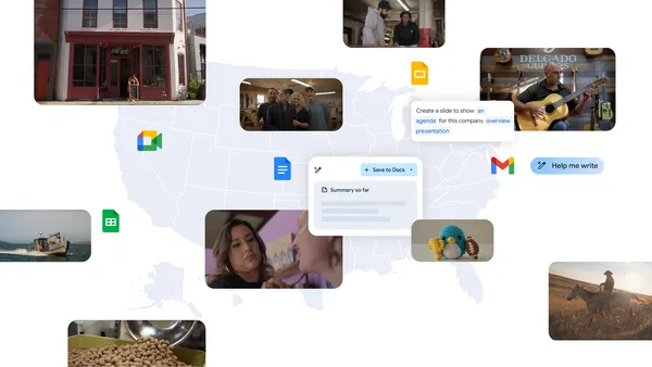
 Learn more about Google’s new local ad spots highlighting small businesses using Gemini for Workspace.Read More
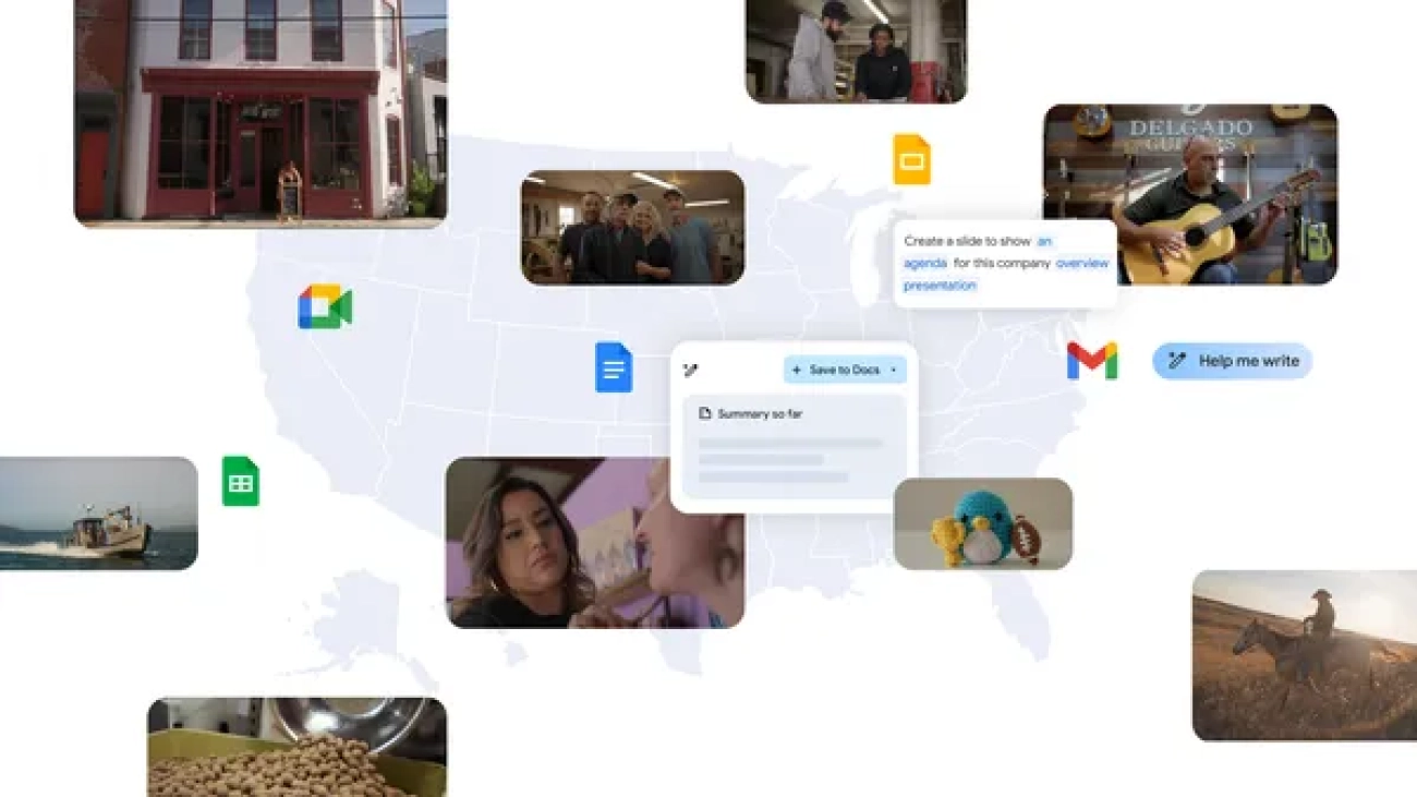
Learn more about Google’s new local ad spots highlighting small businesses using Gemini for Workspace.Read More
 Kent Walker shares three national security imperatives for the AI era.Read More
![]() Learn how Google teams built the Pixel 9 series’ Add Me feature, which uses AI for easier group photos.Read More
Learn how Google teams built the Pixel 9 series’ Add Me feature, which uses AI for easier group photos.Read More
 This post highlights startups in the Google for Startups Growth Academy: AI for Education program, showcasing how artificial intelligence is transforming education.Read More
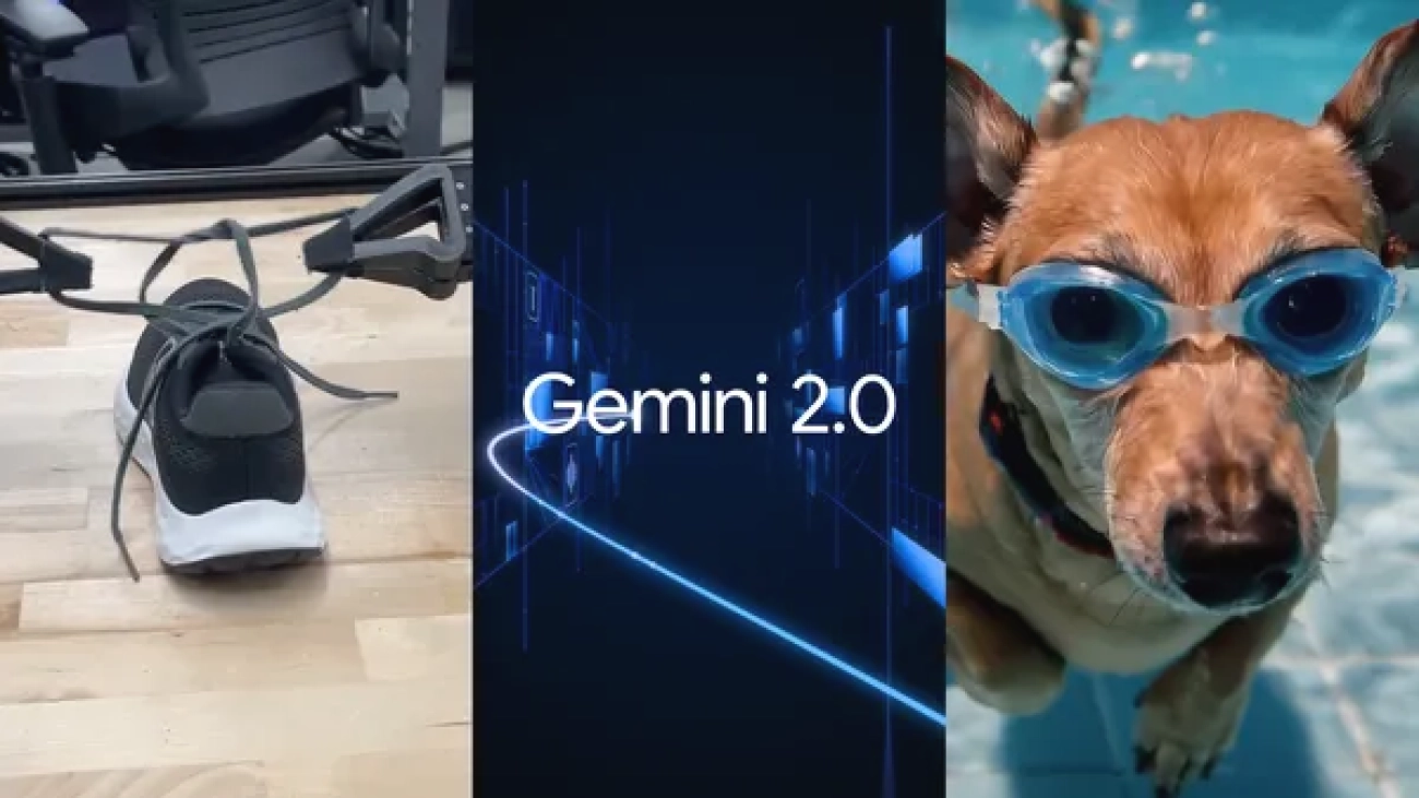
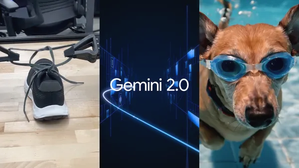 As we move into 2025, we’re looking back at the astonishing progress in AI in 2024.Read More
 New improvements to reporting, controls and creative capabilities are coming to Performance Max.Read More

 The CMA has announced an assessment of whether Google has “Strategic Market Status” (SMS) in the mobile ecosystem under the new Digital Markets, Competition and Consumer…Read More
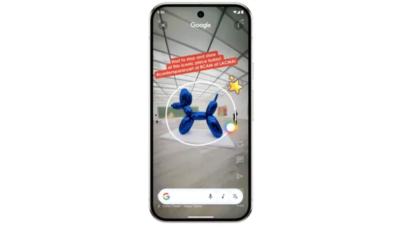
 Last year, we introduced Circle to Search to help you easily circle, scribble or tap anything you see on your Android screen, and find information from the web without s…Read More
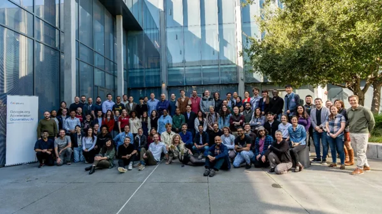
 Apply now for an opportunity to receive funding and to participate in the Google.org Accelerator: Generative AI, a $30 million global open call.Read More
The CMA has announced that it will assess whether Google Search has “Strategic Market Status” (SMS) under the new Digital Markets, Competition and Consumers regime, and …Read More