 Today Google Cloud is unveiling Automotive AI Agent, a new way for automakers to create helpful generative AI experiences. Built using Gemini with Vertex AI, Automotive …Read More

Today Google Cloud is unveiling Automotive AI Agent, a new way for automakers to create helpful generative AI experiences. Built using Gemini with Vertex AI, Automotive …Read More
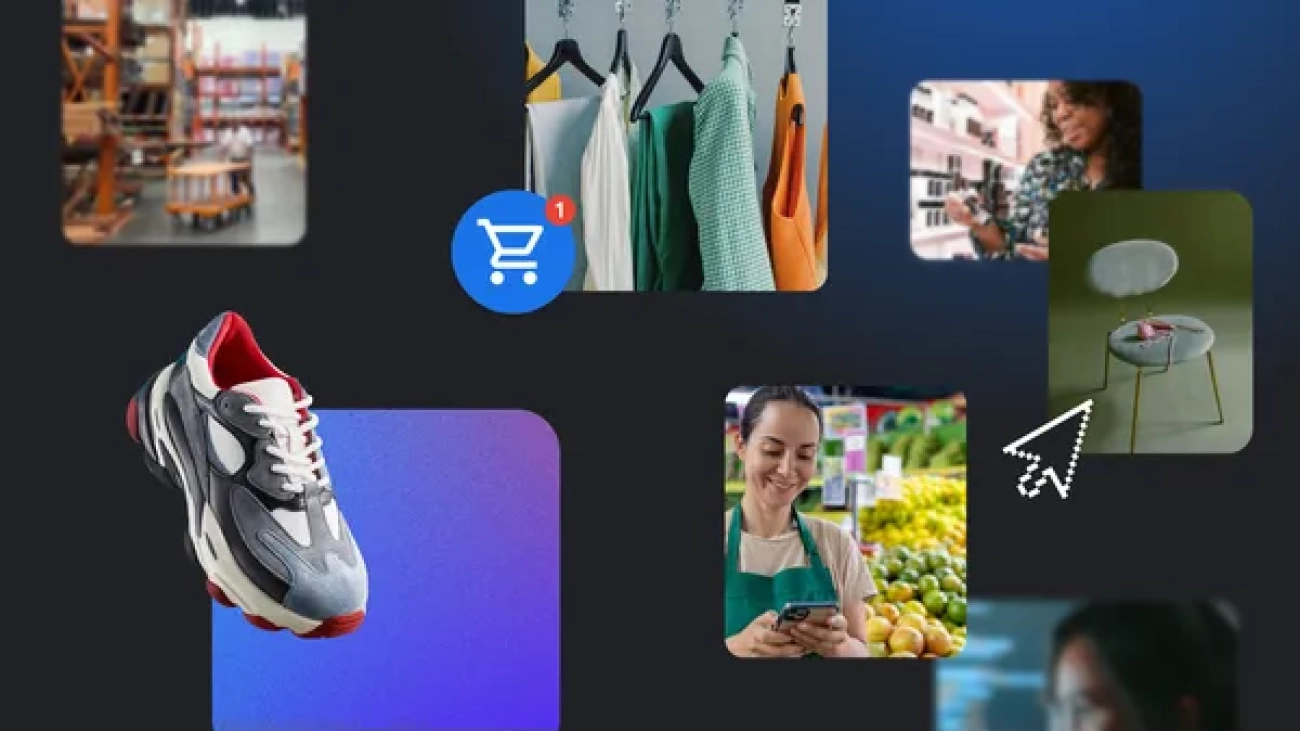
 Learn how retailers are benefiting from Cloud’s gen AI agents, AI-powered search and other AI technology.Read More
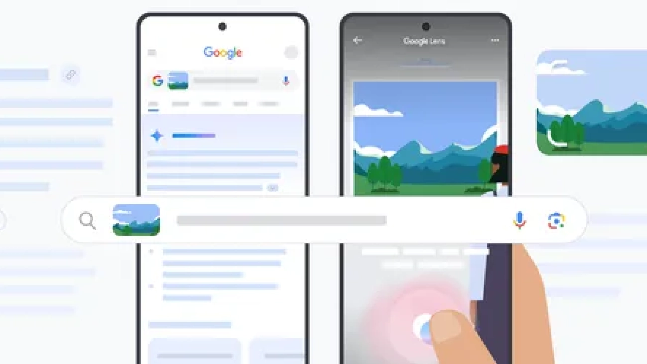
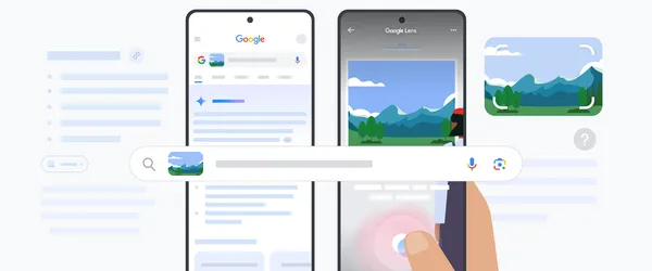 Google Lens uses AI to help you search the world around you. Here’s how to make the most of it.Read More
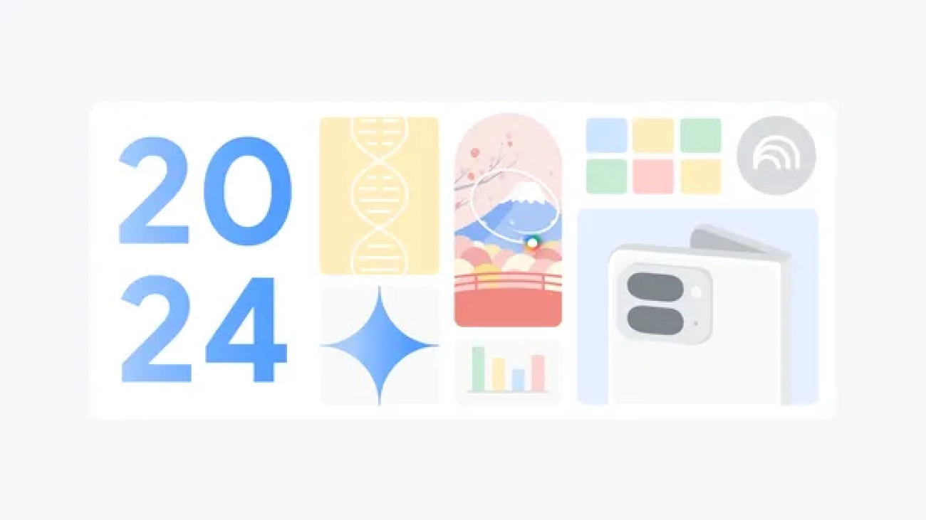
 Recap some of Google’s biggest AI news from 2024, including moments from Gemini, NotebookLM, Search and more.Read More
 Here are Google’s latest AI updates from December including Gemini 2.0, GenCast, and Willow.Read More
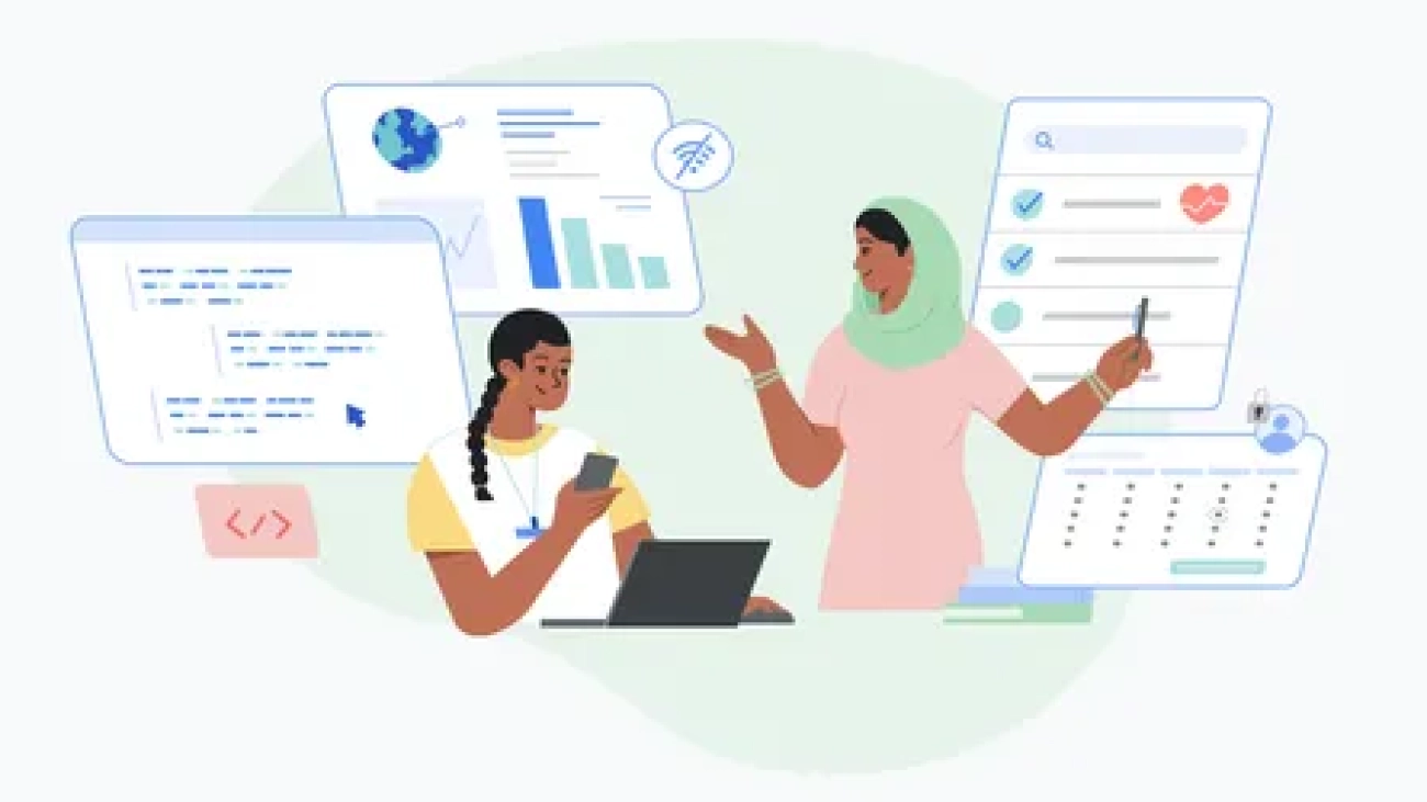
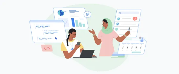 Open Health Stack, a set of open-source tools from Google, allows developers to create digital health solutions for low-resource settings around the world.Read More
 Today we’re refreshing Google’s Generative AI Prohibited Use Policy — the rules of the road that help people use the generative AI tools found in our products and servic…Read More
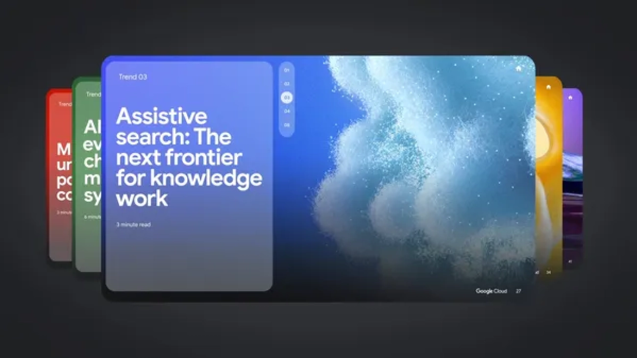
 Learn more about Google Cloud’s AI predictions for businesses in 2025.Read More
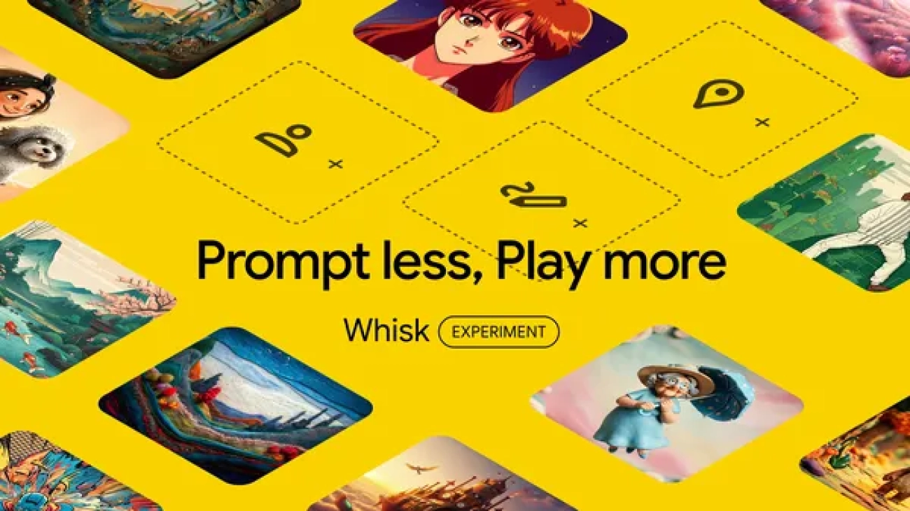
 Whisk is a new Google Labs experiment that lets you prompt using images for a fast and fun creative process.Read More

Whisk is a new Google Labs experiment that lets you prompt using images for a fast and fun creative process.Read More