 Learn more about Google for Startups Accelerator: AI First program for North American startups.Read More
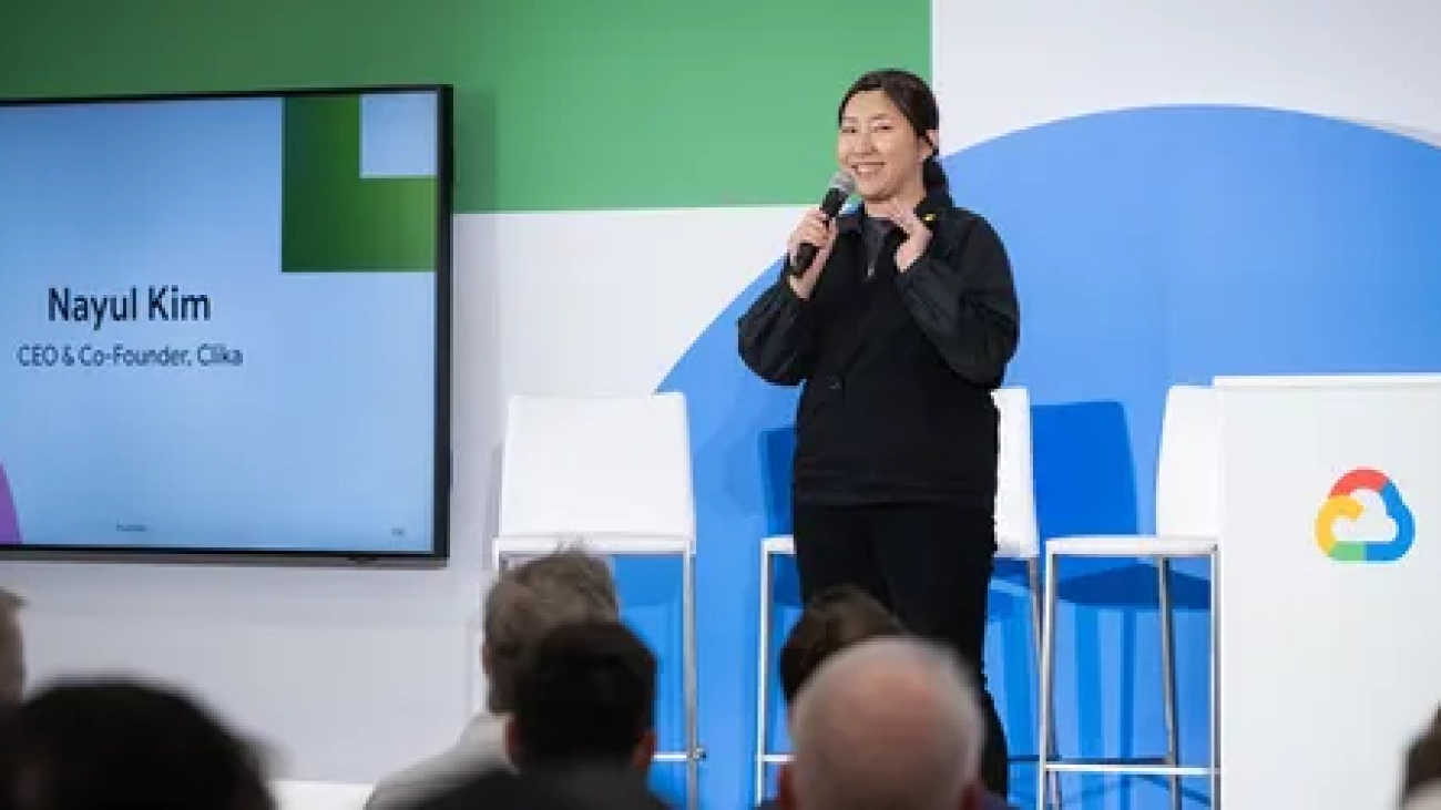
Learn more about Google for Startups Accelerator: AI First program for North American startups.Read More
 Here are Google’s best AI tips and tricks from 2024.Read More

 We commissioned artists Farah Al Qasimi, Charlie Engman and Max Pinckers to envision possible futures with AI for a new exhibition titled “Alternative Images of AI.” Let…Read More
 The Google AI: Release Notes podcast dedicated its most recent episode to the release of Gemini 2.0. Host Logan Kilpatrick chatted with Tulsee Doshi, the head of product…Read More
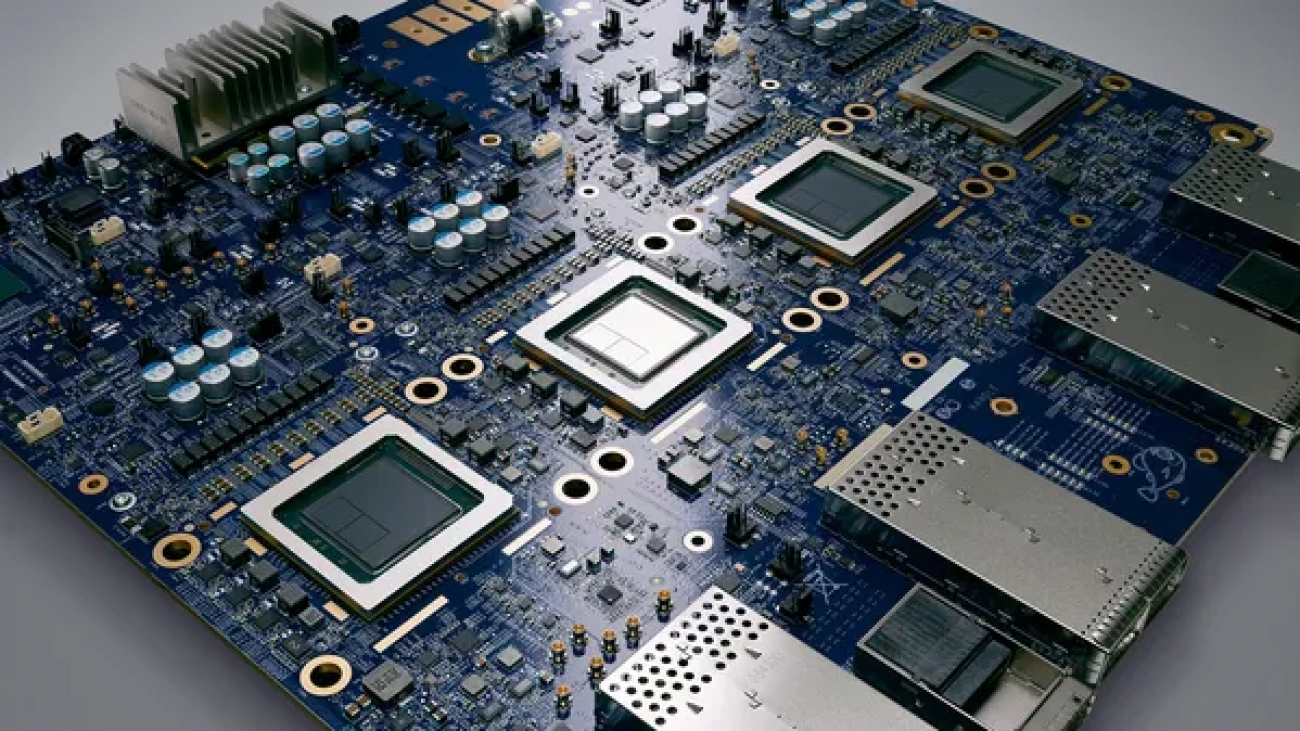
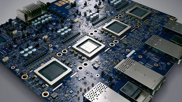 Our sixth-generation Tensor Processing Unit (TPU), called Trillium, is now generally available for Google Cloud customers. The rise of generative AI has created a need f…Read More

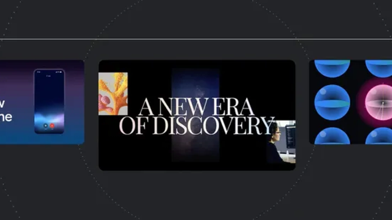
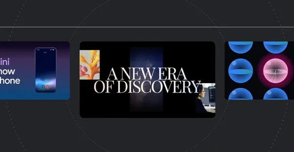
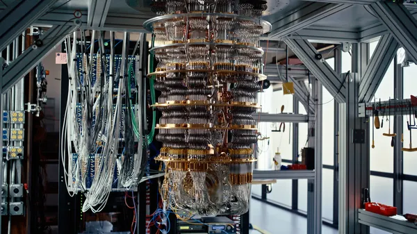 Get a behind-the-scenes look at Google’s Quantum AI lab in Santa Barbara, CA.Read More
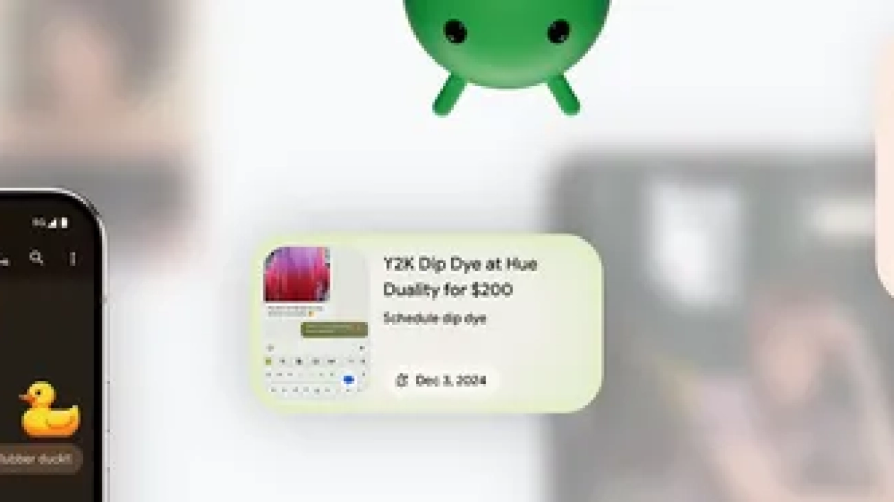
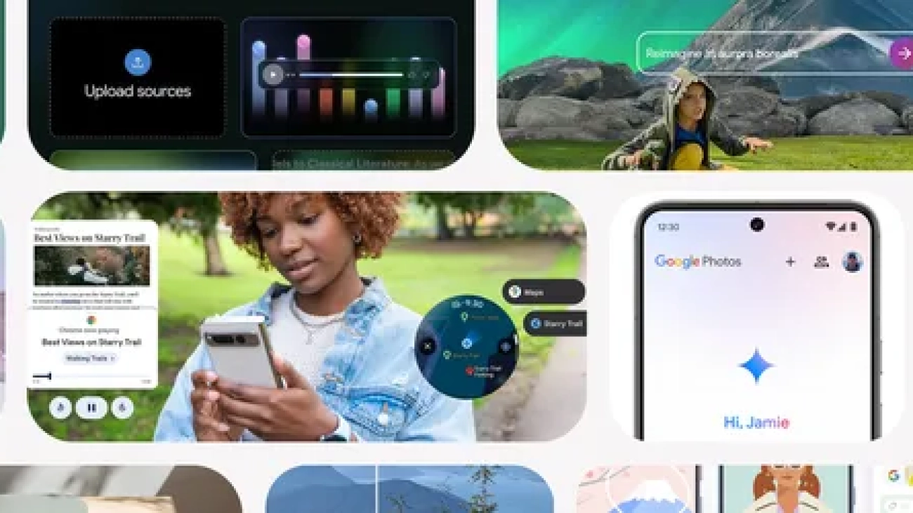
 Learn more about the latest Pixel and Android updates, featuring the latest in Google AI innovation.Read More

 NotebookLM is partnering with Spotify to create a personalized Wrapped AI podcast.Read More
 From a powerful new AI-flood forecasting initiative to help from AI in advancing quantum computers.Read More
 Google and Kaggle recently launched a five-day intensive course about generative AI.Read More