Posts in category: Google AI

Posted by Katherine Heller, Research Scientist, Google Research, on behalf of the CAIR Team

Artificial intelligence (AI) and related machine learning (ML) technologies are increasingly influential in the world around us, making it imperative that we consider the potential impacts on society and individuals in all aspects of the technology that we create. To these ends, the Context in AI Research (CAIR) team develops novel AI methods in the context of the entire AI pipeline: from data to end-user feedback. The pipeline for building an AI system typically starts with data collection, followed by designing a model to run on that data, deployment of the model in the real world, and lastly, compiling and incorporation of human feedback. Originating in the health space, and now expanded to additional areas, the work of the CAIR team impacts every aspect of this pipeline. While specializing in model building, we have a particular focus on building systems with responsibility in mind, including fairness, robustness, transparency, and inclusion.

Data

The CAIR team focuses on understanding the data on which ML systems are built. Improving the standards for the transparency of ML datasets is instrumental in our work. First, we employ documentation frameworks to elucidate dataset and model characteristics as guidance in the development of data and model documentation techniques — Datasheets for Datasets and Model Cards for Model Reporting.

For example, health datasets are highly sensitive and yet can have high impact. For this reason, we developed Healthsheets, a health-contextualized adaptation of a Datasheet. Our motivation for developing a health-specific sheet lies in the limitations of existing regulatory frameworks for AI and health. Recent research suggests that data privacy regulation and standards (e.g., HIPAA, GDPR, California Consumer Privacy Act) do not ensure ethical collection, documentation, and use of data. Healthsheets aim to fill this gap in ethical dataset analysis. The development of Healthsheets was done in collaboration with many stakeholders in relevant job roles, including clinical, legal and regulatory, bioethics, privacy, and product.

Further, we studied how Datasheets and Healthsheets could serve as diagnostic tools that surface the limitations and strengths of datasets. Our aim was to start a conversation in the community and tailor Healthsheets to dynamic healthcare scenarios over time.

To facilitate this effort, we joined the STANDING Together initiative, a consortium that aims to develop international, consensus-based standards for documentation of diversity and representation within health datasets and to provide guidance on how to mitigate risk of bias translating to harm and health inequalities. Being part of this international, interdisciplinary partnership that spans academic, clinical, regulatory, policy, industry, patient, and charitable organizations worldwide enables us to engage in the conversation about responsibility in AI for healthcare internationally. Over 250 stakeholders from across 32 countries have contributed to refining the standards.

Healthsheets and STANDING Together: towards health data documentation and standards.

Model

When ML systems are deployed in the real world, they may fail to behave in expected ways, making poor predictions in new contexts. Such failures can occur for a myriad of reasons and can carry negative consequences, especially within the context of healthcare. Our work aims to identify situations where unexpected model behavior may be discovered, before it becomes a substantial problem, and to mitigate the unexpected and undesired consequences.

Much of the CAIR team’s modeling work focuses on identifying and mitigating when models are underspecified. We show that models that perform well on held-out data drawn from a training domain are not equally robust or fair under distribution shift because the models vary in the extent to which they rely on spurious correlations. This poses a risk to users and practitioners because it can be difficult to anticipate model instability using standard model evaluation practices. We have demonstrated that this concern arises in several domains, including computer vision, natural language processing, medical imaging, and prediction from electronic health records.

We have also shown how to use knowledge of causal mechanisms to diagnose and mitigate fairness and robustness issues in new contexts. Knowledge of causal structure allows practitioners to anticipate the generalizability of fairness properties under distribution shift in real-world medical settings. Further, investigating the capability for specific causal pathways, or “shortcuts”, to introduce bias in ML systems, we demonstrate how to identify cases where shortcut learning leads to predictions in ML systems that are unintentionally dependent on sensitive attributes (e.g., age, sex, race). We have shown how to use causal directed acyclic graphs to adapt ML systems to changing environments under complex forms of distribution shift. Our team is currently investigating how a causal interpretation of different forms of bias, including selection bias, label bias, and measurement error, motivates the design of techniques to mitigate bias during model development and evaluation.

Shortcut Learning: For some models, age may act as a shortcut in classification when using medical images.

The CAIR team focuses on developing methodology to build more inclusive models broadly. For example, we also have work on the design of participatory systems, which allows individuals to choose whether to disclose sensitive attributes, such as race, when an ML system makes predictions. We hope that our methodological research positively impacts the societal understanding of inclusivity in AI method development.

Deployment

The CAIR team aims to build technology that improves the lives of all people through the use of mobile device technology. We aim to reduce suffering from health conditions, address systemic inequality, and enable transparent device-based data collection. As consumer technology, such as fitness trackers and mobile phones, become central in data collection for health, we explored the use of these technologies within the context of chronic disease, in particular, for multiple sclerosis (MS). We developed new data collection mechanisms and predictions that we hope will eventually revolutionize patient’s chronic disease management, clinical trials, medical reversals and drug development.

First, we extended the open-source FDA MyStudies platform, which is used to create clinical study apps, to make it easier for anyone to run their own studies and collect good quality data, in a trusted and safe way. Our improvements include zero-config setups, so that researchers can prototype their study in a day, cross-platform app generation through the use of Flutter and, most importantly, an emphasis on accessibility so that all patient’s voices are heard. We are excited to announce this work has now been open sourced as an extension to the original FDA-Mystudies platform. You can start setting up your own studies today!

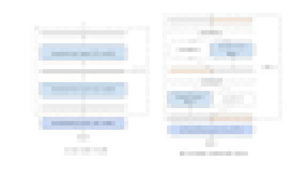
To test this platform, we built a prototype app, which we call MS Signals, that uses surveys to interface with patients in a novel consumer setting. We collaborated with the National MS Society to recruit participants for a user experience study for the app, with the goal of reducing dropout rates and improving the platform further.

MS Signals app screenshots. Left: Study welcome screen. Right: Questionnaire.

Once data is collected, researchers could potentially use it to drive the frontier of ML research in MS. In a separate study, we established a research collaboration with the Duke Department of Neurology and demonstrated that ML models can accurately predict the incidence of high-severity symptoms within three months using continuously collected data from mobile apps. Results suggest that the trained models can be used by clinicians to evaluate the symptom trajectory of MS participants, which may inform decision making for administering interventions.

The CAIR team has been involved in the deployment of many other systems, for both internal and external use. For example, we have also partnered with Learning Ally to build a book recommendation system for children with learning disabilities, such as dyslexia. We hope that our work positively impacts future product development.

Human feedback

As ML models become ubiquitous throughout the developed world, it can be far too easy to leave voices in less developed countries behind. A priority of the CAIR team is to bridge this gap, develop deep relationships with communities, and work together to address ML-related concerns through community-driven approaches.

One of the ways we are doing this is through working with grassroots organizations for ML, such as Sisonkebiotik, an open and inclusive community of researchers, practitioners and enthusiasts at the intersection of ML and healthcare working together to build capacity and drive forward research initiatives in Africa. We worked in collaboration with the Sisonkebiotik community to detail limitations of historical top-down approaches for global health, and suggested complementary health-based methods, specifically those of grassroots participatory communities (GPCs). We jointly created a framework for ML and global health, laying out a practical roadmap towards setting up, growing and maintaining GPCs, based on common values across various GPCs such as Masakhane, Sisonkebiotik and Ro’ya.

We are engaging with open initiatives to better understand the role, perceptions and use cases of AI for health in non-western countries through human feedback, with an initial focus in Africa. Together with Ghana NLP, we have worked to detail the need to better understand algorithmic fairness and bias in health in non-western contexts. We recently launched a study to expand on this work using human feedback.

Biases along the ML pipeline and their associations with African-contextualized axes of disparities.

The CAIR team is committed to creating opportunities to hear more perspectives in AI development. We partnered with Sisonkebiotik to co-organize the Data Science for Health Workshop at Deep Learning Indaba 2023 in Ghana. Everyone’s voice is crucial to developing a better future using AI technology.

Acknowledgements

We would like to thank Negar Rostamzadeh, Stephen Pfohl, Subhrajit Roy, Diana Mincu, Chintan Ghate, Mercy Asiedu, Emily Salkey, Alexander D’Amour, Jessica Schrouff, Chirag Nagpal, Eltayeb Ahmed, Lev Proleev, Natalie Harris, Mohammad Havaei, Ben Hutchinson, Andrew Smart, Awa Dieng, Mahima Pushkarna, Sanmi Koyejo, Kerrie Kauer, Do Hee Park, Lee Hartsell, Jennifer Graves, Berk Ustun, Hailey Joren, Timnit Gebru and Margaret Mitchell for their contributions and influence, as well as our many friends and collaborators at Learning Ally, National MS Society, Duke University Hospital, STANDING Together, Sisonkebiotik, and Masakhane.

Read More

Posted by Kevin Miao and Matt McEwen, Research Scientists, Quantum AI Team

The qubits that make up Google quantum devices are delicate and noisy, so it’s necessary to incorporate error correction procedures that identify and account for qubit errors on the way to building a useful quantum computer. Two of the most prevalent error mechanisms are bit-flip errors (where the energy state of the qubit changes) and phase-flip errors (where the phase of the encoded quantum information changes). Quantum error correction (QEC) promises to address and mitigate these two prominent errors. However, there is an assortment of other error mechanisms that challenges the effectiveness of QEC.

While we want qubits to behave as ideal two-level systems with no loss mechanisms, this is not the case in reality. We use the lowest two energy levels of our qubit (which form the computational basis) to carry out computations. These two levels correspond to the absence (computational ground state) or presence (computational excited state) of an excitation in the qubit, and are labeled |0⟩ (“ket zero”) and |1⟩ (“ket one”), respectively. However, our qubits also host many higher levels called leakage states, which can become occupied. Following the convention of labeling the level by indicating how many excitations are in the qubit, we specify them as |2⟩, |3⟩, |4⟩, and so on.

In “Overcoming leakage in quantum error correction”, published in Nature Physics, we identify when and how our qubits leak energy to higher states, and show that the leaked states can corrupt nearby qubits through our two-qubit gates. We then identify and implement a strategy that can remove leakage and convert it to an error that QEC can efficiently fix. Finally, we show that these operations lead to notably improved performance and stability of the QEC process. This last result is particularly critical, since additional operations take time, usually leading to more errors.

Working with imperfect qubits

Our quantum processors are built from superconducting qubits called transmons. Unlike an ideal qubit, which only has two computational levels — a computational ground state and a computational excited state — transmon qubits have many additional states with higher energy than the computational excited state. These higher leakage states are useful for particular operations that generate entanglement, a necessary resource in quantum algorithms, and also keep transmons from becoming too non-linear and difficult to operate. However, the transmon can also be inadvertently excited into these leakage states through a variety of processes, including imperfections in the control pulses we apply to perform operations or from the small amount of stray heat leftover in our cryogenic refrigerator. These processes are collectively referred to as leakage, which describes the transition of the qubit from computational states to leakage states.

Consider a particular two-qubit operation that is used extensively in our QEC experiments: the CZ gate. This gate operates on two qubits, and when both qubits are in their |1⟩ level, an interaction causes the two individual excitations to briefly “bunch” together in one of the qubits to form |2⟩, while the other qubit becomes |0⟩, before returning to the original configuration where each qubit is in |1⟩. This bunching underlies the entangling power of the CZ gate. However, with a small probability, the gate can encounter an error and the excitations do not return to their original configuration, causing the operation to leave a qubit in |2⟩, a leakage state. When we execute hundreds or more of these CZ gates, this small leakage error probability accumulates.

Transmon qubits support many leakage states (|2⟩, |3⟩, |4⟩, …) beyond the computational basis (|0⟩ and |1⟩). While we typically only use the computational basis to represent quantum information, sometimes the qubit enters these leakage states, and disrupts the normal operation of our qubits.

A single leakage event is especially damaging to normal qubit operation because it induces many individual errors. When one qubit starts in a leaked state, the CZ gate no longer correctly entangles the qubits, preventing the algorithm from executing correctly. Not only that, but CZ gates applied to one qubit in leaked states can cause the other qubit to leak as well, spreading leakage through the device. Our work includes extensive characterization of how leakage is caused and how it interacts with the various operations we use in our quantum processor.

Once the qubit enters a leakage state, it can remain in that state for many operations before relaxing back to the computational states. This means that a single leakage event interferes with many operations on that qubit, creating operational errors that are bunched together in time (time-correlated errors). The ability for leakage to spread between the different qubits in our device through the CZ gates means we also concurrently see bunches of errors on neighboring qubits (space-correlated errors). The fact that leakage induces patterns of space- and time-correlated errors makes it especially hard to diagnose and correct from the perspective of QEC algorithms.

The effect of leakage in QEC

We aim to mitigate qubit errors by implementing surface code QEC, a set of operations applied to a collection of imperfect physical qubits to form a logical qubit, which has properties much closer to an ideal qubit. In a nutshell, we use a set of qubits called data qubits to hold the quantum information, while another set of measure qubits check up on the data qubits, reporting on whether they have suffered any errors, without destroying the delicate quantum state of the data qubits. One of the key underlying assumptions of QEC is that errors occur independently for each operation, but leakage can persist over many operations and cause a correlated pattern of multiple errors. The performance of our QEC strategies is significantly limited when leakage causes this assumption to be violated.

Once leakage manifests in our surface code transmon grid, it persists for a long time relative to a single surface code QEC cycle. To make matters worse, leakage on one qubit can cause its neighbors to leak as well.

Our previous work has shown that we can remove leakage from measure qubits using an operation called multi-level reset (MLR). This is possible because once we perform a measurement on measure qubits, they no longer hold any important quantum information. At this point, we can interact the qubit with a very lossy frequency band, causing whichever state the qubit was in (including leakage states) to decay to the computational ground state |0⟩. If we picture a Jenga tower representing the excitations in the qubit, we tumble the entire stack over. Removing just one brick, however, is much more challenging. Likewise, MLR doesn’t work with data qubits because they always hold important quantum information, so we need a new leakage removal approach that minimally disturbs the computational basis states.

Gently removing leakage

We introduce a new quantum operation called data qubit leakage removal (DQLR), which targets leakage states in a data qubit and converts them into computational states in the data qubit and a neighboring measure qubit. DQLR consists of a two-qubit gate (dubbed Leakage iSWAP — an iSWAP operation with leakage states) inspired by and similar to our CZ gate, followed by a rapid reset of the measure qubit to further remove errors. The Leakage iSWAP gate is very efficient and greatly benefits from our extensive characterization and calibration of CZ gates within the surface code experiment.

Recall that a CZ gate takes two single excitations on two different qubits and briefly brings them to one qubit, before returning them to their respective qubits. A Leakage iSWAP gate operates similarly, but almost in reverse, so that it takes a single qubit with two excitations (otherwise known as |2⟩) and splits them into |1⟩ on two qubits. The Leakage iSWAP gate (and for that matter, the CZ gate) is particularly effective because it does not operate on the qubits if there are fewer than two excitations present. We are precisely removing the |2⟩ Jenga brick without toppling the entire tower.

By carefully measuring the population of leakage states on our transmon grid, we find that DQLR can reduce average leakage state populations over all qubits to about 0.1%, compared to nearly 1% without it. Importantly, we no longer observe a gradual rise in the amount of leakage on the data qubits, which was always present to some extent prior to using DQLR.

This outcome, however, is only half of the puzzle. As mentioned earlier, an operation such as MLR could be used to effectively remove leakage on the data qubits, but it would also completely erase the stored quantum state. We also need to demonstrate that DQLR is compatible with the preservation of a logical quantum state.

The second half of the puzzle comes from executing the QEC experiment with this operation interleaved at the end of each QEC cycle, and observing the logical performance. Here, we use a metric called detection probability to gauge how well we are executing QEC. In the presence of leakage, time- and space-correlated errors will cause a gradual rise in detection probabilities as more and more qubits enter and stay in leakage states. This is most evident when we perform no reset at all, which rapidly leads to a transmon grid plagued by leakage, and it becomes inoperable for the purposes of QEC.

The prior state-of-the-art in our QEC experiments was to use MLR on the measure qubits to remove leakage. While this kept leakage population on the measure qubits (green circles) sufficiently low, data qubit leakage population (green squares) would grow and saturate to a few percent. With DQLR, leakage population on both the measure (blue circles) and data qubits (blue squares) remain acceptably low and stable.

With MLR, the large reduction in leakage population on the measure qubits drastically decreases detection probabilities and mitigates a considerable degree of the gradual rise. This reduction in detection probability happens even though we spend more time dedicated to the MLR gate, when other errors can potentially occur. Put another way, the correlated errors that leakage causes on the grid can be much more damaging than the uncorrelated errors from the qubits waiting idle, and it is well worth it for us to trade the former for the latter.

When only using MLR, we observed a small but persistent residual rise in detection probabilities. We ascribed this residual increase in detection probability to leakage accumulating on the data qubits, and found that it disappeared when we implemented DQLR. And again, the observation that the detection probabilities end up lower compared to only using MLR indicates that our added operation has removed a damaging error mechanism while minimally introducing uncorrelated errors.

Leakage manifests during surface code operation as increased errors (shown as error detection probabilities) over the number of cycles. With DQLR, we no longer see a notable rise in detection probability over more surface code cycles.

Prospects for QEC scale-up

Given these promising results, we are eager to implement DQLR in future QEC experiments, where we expect error mechanisms outside of leakage to be greatly improved, and sensitivity to leakage to be enhanced as we work with larger and larger transmon grids. In particular, our simulations indicate that scale-up of our surface code will almost certainly require a large reduction in leakage generation rates, or an active leakage removal technique over all qubits, such as DQLR.

Having laid the groundwork by understanding where leakage is generated, capturing the dynamics of leakage after it presents itself in a transmon grid, and showing that we have an effective mitigation strategy in DQLR, we believe that leakage and its associated errors no longer pose an existential threat to the prospects of executing a surface code QEC protocol on a large grid of transmon qubits. With one fewer challenge standing in the way of demonstrating working QEC, the pathway to a useful quantum computer has never been more promising.

Acknowledgements

This work would not have been possible without the contributions of the entire Google Quantum AI Team.

Read More

Generative AI in Search, or Search Generative Experience (SGE), is expanding around the world, and adding four new languages.Read More

Today, we’re announcing the Swedish recipients of Google.org Impact Challenge: Tech for Social Good – receiving technical support and 3 million Euros in funding for char…Read More

Posted by Xin Wang, Software Engineer, and Nishanth Dikkala, Research Scientist, Google Research

Contemporary deep learning models have been remarkably successful in many domains, ranging from natural language to computer vision. Transformer neural networks (transformers) are a popular deep learning architecture that today comprise the foundation for most tasks in natural language processing and also are starting to extend to applications in other domains, such as computer vision, robotics, and autonomous driving. Moreover, they form the backbone of all the current state-of-the-art language models.

Increasing scale in Transformer networks has led to improved performance and the emergence of behavior not present in smaller networks. However, this increase in scale often comes with prohibitive increases in compute cost and inference latency. A natural question is whether we can reap the benefits of larger models without incurring the computational burden.

In “Alternating Updates for Efficient Transformers”, accepted as a Spotlight at NeurIPS 2023, we introduce AltUp, a method to take advantage of increased token representation without increasing the computation cost. AltUp is easy to implement, widely applicable to any transformer architecture, and requires minimal hyperparameter tuning. For instance, using a variant of AltUp on a 770M parameter T5-Large model, the addition of ~100 parameters yields a model with a significantly better quality.

Background

To understand how we can achieve this, we dig into how transformers work. First, they partition the input into a sequence of tokens. Each token is then mapped to an embedding vector (via the means of an embedding table) called the token embedding. We call the dimension of this vector the token representation dimension. The Transformer then operates on this sequence of token embeddings by applying a series of computation modules (called layers) using its network parameters. The number of parameters in each transformer layer is a function of the layer’s width, which is determined by the token representation dimension.

To achieve benefits of scale without incurring the compute burden, prior works such as sparse mixture-of-experts (Sparse MoE) models (e.g., Switch Transformer, Expert Choice, V-MoE) have predominantly focused on efficiently scaling up the network parameters (in the self-attention and feedforward layers) by conditionally activating a subset based on the input. This allows us to scale up network size without significantly increasing compute per input. However, there is a research gap on scaling up the token representation dimension itself by conditionally activating parts of the token representation vector.

Recent works (for example, scaling laws and infinite-width networks) have empirically and theoretically established that a wider token representation helps in learning more complicated functions. This phenomenon is also evident in modern architectures of increasing capability. For instance, the representation dimension grows from 512 (small) to 768 (base) and 1024 (corresponding to models with 770M, 3B, and 11B parameters respectively) in T5 models, and from 4096 (8B) to 8192 (64B) and 18432 (540B) in PaLM models. A widened representation dimension also significantly improves performance for dual encoder retrieval models. However, naïvely widening the representation vector requires one to increase the model dimension accordingly, which quadratically¹ increases the amount of computation in the feedforward computation.

Method

AltUp works by partitioning a widened representation vector into equal sized blocks, processing only a single block at each layer, and using an efficient prediction-correction mechanism to infer the outputs of the other blocks (shown below on the right). This allows AltUp to simultaneously keep the model dimension, hence the computation cost, roughly constant and take advantage of using an increased token dimension. The increased token dimension allows the model to pack more information into each token’s embedding. By keeping the width of each transformer layer constant, AltUp avoids incurring the quadratic increase in computation cost that would otherwise be present with a naïve expansion of the representation.

An illustration of widening the token representation without (left) and with AltUp (right). This widening causes a near-quadratic increase in computation in a vanilla transformer due to the increased layer width. In contrast, Alternating Updates keeps the layer width constant and efficiently computes the output by operating on a sub-block of the representation at each layer.

More specifically, the input to each layer is two or more blocks, one of which is passed into the 1x width transformer layer (see figure below). We refer to this block as the “activated” block. This computation results in the exact output for the activated block. In parallel, we invoke a lightweight predictor that computes a weighted combination of all the input blocks. The predicted values, along with the computed value of the activated block, are passed on to a lightweight corrector that updates the predictions based on the observed values. This correction mechanism enables the inactivated blocks to be updated as a function of the activated one. Both the prediction and correction steps only involve a limited number of vector additions and multiplications and hence are much faster than a regular transformer layer. We note that this procedure can be generalized to an arbitrary number of blocks.

The predictor and corrector computations: The predictor mixes sub-blocks with trainable scalar coefficients; the corrector returns a weighted average of the predictor output and the transformer output. The predictor and corrector perform scalar-vector multiplications and incur negligible computation cost compared to the transformer. The predictor outputs a linear mixing of blocks with scalar mixing coefficients pi, j , and the corrector combines predictor output and transformer output with weights gi.

At a higher level, AltUp is similar to sparse MoE in that it is a method to add capacity to a model in the form of conditionally accessed (external) parameters. In sparse MoE, the additional parameters take the form of feed forward network (FFN) experts and the conditionality is with respect to the input. In AltUp, the external parameters come from the widened embedding table and the conditionality takes the form of alternating block-wise activation of the representation vector, as in the figure above. Hence, AltUp has the same underpinning as sparse MoE models.

An advantage of AltUp over sparse MoE is that it does not necessitate sharding since the number of additional parameters introduced is a factor² of the embedding table size, which typically makes up a small fraction of the overall model size. Moreover, since AltUp focuses on conditionally activating parts of a wider token representation, it can be applied synergistically with orthogonal techniques like MoE to obtain complementary performance gains.

Evaluation

AltUp was evaluated on T5 models on various benchmark language tasks. Models augmented with AltUp are uniformly faster than the extrapolated dense models at the same accuracy. For example, we observe that a T5 Large model augmented with AltUp leads to a 27%, 39%, 87%, and 29% speedup on GLUE, SuperGLUE, SQuAD, and Trivia-QA benchmarks, respectively.

Evaluations of AltUp on T5 models of various sizes and popular benchmarks. AltUp consistently leads to sizable speedups relative to baselines at the same accuracy. Latency is measured on TPUv3 with 8 cores. Speedup is defined as the change in latency divided by the AltUp latency (B = T5 Base, L = T5 Large, XL = T5 XL models).

AltUp’s relative performance improves as we apply it to larger models — compare the relative speedup of T5 Base + AltUp to that of T5 Large + AltUp. This demonstrates the scalability of AltUp and its improved performance on even larger models. Overall, AltUp consistently leads to models with better predictive performance than the corresponding baseline models with the same speed on all evaluated model sizes and benchmarks.

Extensions: Recycled AltUp

The AltUp formulation adds an insignificant amount of per-layer computation, however, it does require using a wider embedding table. In certain scenarios where the vocabulary size (i.e., the number of distinct tokens the tokenizer can produce) is very large, this may lead to a non-trivial amount of added computation for the initial embedding lookup and the final linear + softmax operation. A very large vocabulary may also lead to an undesirable amount of added embedding parameters. To address this, Recycled-AltUp is an extension of AltUp that avoids these computational and parameter costs by keeping the embedding table’s width the same.

Illustration of the Architecture for Recycled-AltUp with K = 2.

In Recycled-AltUp, instead of widening the initial token embeddings, we replicate the embeddings K times to form a wider token representation. Hence, Recycled-AltUp adds virtually no additional parameters relative to the baseline transformer, while benefiting from a wider token representation.

Recycled-AltUp on T5-B/L/XL compared to baselines. Recycled-AltUp leads to strict improvements in pre-training performance without incurring any perceptible slowdown.

We also evaluate the lightweight extension of AltUp, Recycled-AltUp, with K = 2 on T5 base, large, and XL models and compare its pre-trained accuracy and speed to those of baselines. Since Recycled-AltUp does not require an expansion in the embedding table dimension, the models augmented with it have virtually the same number of trainable parameters as the baseline models. We again observe consistent improvements compared to the dense baselines.

Why does AltUp work?

AltUp increases a model’s capacity by adding and efficiently leveraging auxiliary parameters to the embedding table, and maintaining the higher dimensional representation across the layers. We believe that a key ingredient in this computation lies in AltUp’s prediction mechanism that performs an ensemble of the different blocks. This weighted combination enables continuous message passing to the entire vector despite activating only sub-blocks of it in each layer. Recycled-AltUp, on the other hand, does not add any additional parameters to the token embeddings. However, it still confers the benefit of simulating computation in a higher dimensional representation space since a higher dimensional representation vector is maintained when moving from one transformer layer to another. We conjecture that this aids the training by augmenting the flow of information through the network. An interesting research direction is to explore whether the benefits of Recycled-AltUp can be explained entirely by more favorable training dynamics.

Acknowledgements

We thank our collaborators Cenk Baykal, Dylan Cutler, and Rina Panigrahy at Google Research, and Nikhil Ghosh at University of California, Berkeley (work done during research internship at Google).

¹This is because the feedforward layers of a Transformer are typically scaled quadratically with the model dimension. <sup>↩

2</sup>This factor depends on the user-specified expansion factor, but is typically 1, i.e., we double the embedding table dimension. ^↩

Read More

Posted by Sara Ahmadian and Mehran Kazemi, Research Scientists, Google Research

Clustering is a fundamental, ubiquitous problem in data mining and unsupervised machine learning, where the goal is to group together similar items. The standard forms of clustering are metric clustering and graph clustering. In metric clustering, a given metric space defines distances between data points, which are grouped together based on their separation. In graph clustering, a given graph connects similar data points through edges, and the clustering process groups data points together based on the connections between them. Both clustering forms are particularly useful for large corpora where class labels can’t be defined. Examples of such corpora are the ever-growing digital text collections of various internet platforms, with applications including organizing and searching documents, identifying patterns in text, and recommending relevant documents to users (see more examples in the following posts: clustering related queries based on user intent and practical differentially private clustering).

The choice of text clustering method often presents a dilemma. One approach is to use embedding models, such as BERT or RoBERTa, to define a metric clustering problem. Another is to utilize cross-attention (CA) models, such as PaLM or GPT, to define a graph clustering problem. CA models can provide highly accurate similarity scores, but constructing the input graph may require a prohibitive quadratic number of inference calls to the model. On the other hand, a metric space can efficiently be defined by distances of embeddings produced by embedding models. However, these similarity distances are typically of substantial lower-quality compared to the similarity signals of CA models, and hence the produced clustering can be of much lower-quality.

Motivated by this, in “KwikBucks: Correlation Clustering with Cheap-Weak and Expensive-Strong Signals”, presented at ICLR 2023, we describe a novel clustering algorithm that effectively combines the scalability benefits from embedding models and the quality from CA models. This graph clustering algorithm has query access to both the CA model and the embedding model, however, we apply a budget on the number of queries made to the CA model. This algorithm uses the CA model to answer edge queries, and benefits from unlimited access to similarity scores from the embedding model. We describe how this proposed setting bridges algorithm design and practical considerations, and can be applied to other clustering problems with similar available scoring functions, such as clustering problems on images and media. We demonstrate how this algorithm yields high-quality clusters with almost a linear number of query calls to the CA model. We have also open-sourced the data used in our experiments.

The clustering algorithm

The KwikBucks algorithm is an extension of the well-known KwikCluster algorithm (Pivot algorithm). The high-level idea is to first select a set of documents (i.e., centers) with no similarity edge between them, and then form clusters around these centers. To obtain the quality from CA models and the runtime efficiency from embedding models, we introduce the novel combo similarity oracle mechanism. In this approach, we utilize the embedding model to guide the selection of queries to be sent to the CA model. When given a set of center documents and a target document, the combo similarity oracle mechanism outputs a center from the set that is similar to the target document, if present. The combo similarity oracle enables us to save on budget by limiting the number of query calls to the CA model when selecting centers and forming clusters. It does this by first ranking centers based on their embedding similarity to the target document, and then querying the CA model for the pair (i.e., target document and ranked center), as shown below.

A combo similarity oracle that for a set of documents and a target document, returns a similar document from the set, if present.

We then perform a post processing step to merge clusters if there is a strong connection between two of them, i.e., when the number of connecting edges is higher than the number of missing edges between two clusters. Additionally, we apply the following steps for further computational savings on queries made to the CA model, and to improve performance at runtime:

1. We leverage query-efficient correlation clustering to form a set of centers from a set of randomly selected documents instead of selecting these centers from all the documents (in the illustration below, the center nodes are red).
2. We apply the combo similarity oracle mechanism to perform the cluster assignment step in parallel for all non-center documents and leave documents with no similar center as singletons. In the illustration below, the assignments are depicted by blue arrows and initially two (non-center) nodes are left as singletons due to no assignment.
3. In the post-processing step, to ensure scalability, we use the embedding similarity scores to filter down the potential mergers (in the illustration below, the green dashed boundaries show these merged clusters).

Illustration of progress of the clustering algorithm on a given graph instance.

Results

We evaluate the novel clustering algorithm on various datasets with different properties using different embedding-based and cross-attention–based models. We compare the clustering algorithm’s performance with the two best performing baselines (see the paper for more details):

• The query-efficient correlation clustering algorithm for budgeted clustering with access to CA only.
• Spectral clustering on the k-nearest neighbor graph (kNN) formed by querying the CA model for the k-nearest neighbors of each vertex from embedding-based similarity.

To evaluate the quality of clustering, we use precision and recall. Precision is used to calculate the percentage of similar pairs out of all co-clustered pairs and recall is the percentage of co-clustered similar pairs out of all similar pairs. To measure the quality of the obtained solutions from our experiments, we use the F1-score, which is the harmonic mean of the precision and recall, where 1.0 is the highest possible value that indicates perfect precision and recall, and 0 is the lowest possible value that indicates if either precision or recall are zero. The table below reports the F1-score for Kwikbucks and various baselines in the case that we allow only a linear number of queries to the CA model. We show that Kwikbucks offers a substantial boost in performance with a 45% relative improvement compared to the best baseline when averaging across all datasets.

Comparing the clustering algorithm to two baseline algorithms using various public datasets: (1) The query-efficient correlation clustering algorithm for budgeted clustering with access to CA only, and (2) spectral clustering on the k-nearest neighbor (kNN) graph formed by querying the CA model for the k-nearest neighbors of each vertex from embedding-based similarity. Pre-processed datasets can be downloaded here.

The figure below compares the clustering algorithm’s performance with baselines using different query budgets. We observe that KwikBucks consistently outperforms other baselines at various budgets.

A comparison of KwikBucks with top-2 baselines when allowed different budgets for querying the cross-attention model.

Conclusion

Text clustering often presents a dilemma in the choice of similarity function: embedding models are scalable but lack quality, while cross-attention models offer quality but substantially hurt scalability. We present a clustering algorithm that offers the best of both worlds: the scalability of embedding models and the quality of cross-attention models. KwikBucks can also be applied to other clustering problems with multiple similarity oracles of varying accuracy levels. This is validated with an exhaustive set of experiments on various datasets with diverse properties. See the paper for more details.

Acknowledgements

This project was initiated during Sandeep Silwal’s summer internship at Google in 2022. We would like to express our gratitude to our co-authors, Andrew McCallum, Andrew Nystrom, Deepak Ramachandran, and Sandeep Silwal, for their valuable contributions to this work. We also thank Ravi Kumar and John Guilyard for assistance with this blog post.

Read More

Posted by Xingchen Wan, Student Researcher, and Ruoxi Sun, Research Scientist, Cloud AI Team

Recent advances in large language models (LLMs) are very promising as reflected in their capability for general problem-solving in few-shot and zero-shot setups, even without explicit training on these tasks. This is impressive because in the few-shot setup, LLMs are presented with only a few question-answer demonstrations prior to being given a test question. Even more challenging is the zero-shot setup, where the LLM is directly prompted with the test question only.

Even though the few-shot setup has dramatically reduced the amount of data required to adapt a model for a specific use-case, there are still cases where generating sample prompts can be challenging. For example, handcrafting even a small number of demos for the broad range of tasks covered by general-purpose models can be difficult or, for unseen tasks, impossible. For example, for tasks like summarization of long articles or those that require domain knowledge (e.g., medical question answering), it can be challenging to generate sample answers. In such situations, models with high zero-shot performance are useful since no manual prompt generation is required. However, zero-shot performance is typically weaker as the LLM is not presented with guidance and thus is prone to spurious output.

In “Better Zero-shot Reasoning with Self-Adaptive Prompting”, published at ACL 2023, we propose Consistency-Based Self-Adaptive Prompting (COSP) to address this dilemma. COSP is a zero-shot automatic prompting method for reasoning problems that carefully selects and constructs pseudo-demonstrations for LLMs using only unlabeled samples (that are typically easy to obtain) and the models’ own predictions. With COSP, we largely close the performance gap between zero-shot and few-shot while retaining the desirable generality of zero-shot prompting. We follow this with “Universal Self-Adaptive Prompting“ (USP), accepted at EMNLP 2023, in which we extend the idea to a wide range of general natural language understanding (NLU) and natural language generation (NLG) tasks and demonstrate its effectiveness.

Prompting LLMs with their own outputs

Knowing that LLMs benefit from demonstrations and have at least some zero-shot abilities, we wondered whether the model’s zero-shot outputs could serve as demonstrations for the model to prompt itself. The challenge is that zero-shot solutions are imperfect, and we risk giving LLMs poor quality demonstrations, which could be worse than no demonstrations at all. Indeed, the figure below shows that adding a correct demonstration to a question can lead to a correct solution of the test question (Demo1 with question), whereas adding an incorrect demonstration (Demo 2 + questions, Demo 3 with questions) leads to incorrect answers. Therefore, we need to select reliable self-generated demonstrations.

Example inputs & outputs for reasoning tasks, which illustrates the need for carefully designed selection procedure for in-context demonstrations (MultiArith dataset & PaLM-62B model): (1) zero-shot chain-of-thought with no demo: correct logic but wrong answer; (2) correct demo (Demo1) and correct answer; (3) correct but repetitive demo (Demo2) leads to repetitive outputs; (4) erroneous demo (Demo3) leads to a wrong answer; but (5) combining Demo3 and Demo1 again leads to a correct answer.

COSP leverages a key observation of LLMs: that confident and consistent predictions are more likely correct. This observation, of course, depends on how good the uncertainty estimate of the LLM is. Luckily, in large models, previous works suggest that the uncertainty estimates are robust. Since measuring confidence requires only model predictions, not labels, we propose to use this as a zero-shot proxy of correctness. The high-confidence outputs and their inputs are then used as pseudo-demonstrations.

With this as our starting premise, we estimate the model’s confidence in its output based on its self-consistency and use this measure to select robust self-generated demonstrations. We ask LLMs the same question multiple times with zero-shot chain-of-thought (CoT) prompting. To guide the model to generate a range of possible rationales and final answers, we include randomness controlled by a “temperature” hyperparameter. In an extreme case, if the model is 100% certain, it should output identical final answers each time. We then compute the entropy of the answers to gauge the uncertainty — the answers that have high self-consistency and for which the LLM is more certain, are likely to be correct and will be selected.

Assuming that we are presented with a collection of unlabeled questions, the COSP method is:

1. Input each unlabeled question into an LLM, obtaining multiple rationales and answers by sampling the model multiple times. The most frequent answers are highlighted, followed by a score that measures consistency of answers across multiple sampled outputs (higher is better). In addition to favoring more consistent answers, we also penalize repetition within a response (i.e., with repeated words or phrases) and encourage diversity of selected demonstrations. We encode the preference towards consistent, un-repetitive and diverse outputs in the form of a scoring function that consists of a weighted sum of the three scores for selection of the self-generated pseudo-demonstrations.
2. We concatenate the pseudo-demonstrations into test questions, feed them to the LLM, and obtain a final predicted answer.

Illustration of COSP: In Stage 1 (left), we run zero-shot CoT multiple times to generate a pool of demonstrations (each consisting of the question, generated rationale and prediction) and assign a score. In Stage 2 (right), we augment the current test question with pseudo-demos (blue boxes) and query the LLM again. A majority vote over outputs from both stages forms the final prediction.

COSP focuses on question-answering tasks with CoT prompting for which it is easy to measure self-consistency since the questions have unique correct answers. But this can be difficult for other tasks, such as open-ended question-answering or generative tasks that don’t have unique answers (e.g., text summarization). To address this limitation, we introduce USP in which we generalize our approach to other general NLP tasks:

• Classification (CLS): Problems where we can compute the probability of each class using the neural network output logits of each class. In this way, we can measure the uncertainty without multiple sampling by computing the entropy of the logit distribution.
• Short-form generation (SFG): Problems like question answering where we can use the same procedure mentioned above for COSP, but, if necessary, without the rationale-generating step.
• Long-form generation (LFG): Problems like summarization and translation, where the questions are often open-ended and the outputs are unlikely to be identical, even if the LLM is certain. In this case, we use an overlap metric in which we compute the average of the pairwise ROUGE score between the different outputs to the same query.

Illustration of USP in exemplary tasks (classification, QA and text summarization). Similar to COSP, the LLM first generates predictions on an unlabeled dataset whose outputs are scored with logit entropy, consistency or alignment, depending on the task type, and pseudo-demonstrations are selected from these input-output pairs. In Stage 2, the test instances are augmented with pseudo-demos for prediction.

We compute the relevant confidence scores depending on the type of task on the aforementioned set of unlabeled test samples. After scoring, similar to COSP, we pick the confident, diverse and less repetitive answers to form a model-generated pseudo-demonstration set. We finally query the LLM again in a few-shot format with these pseudo-demonstrations to obtain the final predictions on the entire test set.

Key Results

For COSP, we focus on a set of six arithmetic and commonsense reasoning problems, and we compare against 0-shot-CoT (i.e., “Let’s think step by step“ only). We use self-consistency in all baselines so that they use roughly the same amount of computational resources as COSP. Compared across three LLMs, we see that zero-shot COSP significantly outperforms the standard zero-shot baseline.

Key results of COSP in six arithmetic (MultiArith, GSM-8K, AddSub, SingleEq) and commonsense (CommonsenseQA, StrategyQA) reasoning tasks using PaLM-62B, PaLM-540B and GPT-3 (code-davinci-001) models.

USP improves significantly on 0-shot performance. “CLS” is an average of 15 classification tasks; “SFG” is the average of five short-form generation tasks; “LFG” is the average of two summarization tasks. “SFG (BBH)” is an average of all BIG-Bench Hard tasks, where each question is in SFG format.

For USP, we expand our analysis to a much wider range of tasks, including more than 25 classifications, short-form generation, and long-form generation tasks. Using the state-of-the-art PaLM 2 models, we also test against the BIG-Bench Hard suite of tasks where LLMs have previously underperformed compared to people. We show that in all cases, USP again outperforms the baselines and is competitive to prompting with golden examples.

Accuracy on BIG-Bench Hard tasks with PaLM 2-M (each line represents a task of the suite). The gain/loss of USP (green stars) over standard 0-shot (green triangles) is shown in percentages. “Human” refers to average human performance; “AutoCoT” and “Random demo” are baselines we compared against in the paper; and “3-shot” is the few-shot performance for three handcrafted demos in CoT format.

We also analyze the working mechanism of USP by validating the key observation above on the relation between confidence and correctness, and we found that in an overwhelming majority of the cases, USP picks confident predictions that are more likely better in all task types considered, as shown in the figure below.

USP picks confident predictions that are more likely better. Ground-truth performance metrics against USP confidence scores in selected tasks in various task types (blue: CLS, orange: SFG, green: LFG) with PaLM-540B.

Conclusion

Zero-shot inference is a highly sought-after capability of modern LLMs, yet the success in which poses unique challenges. We propose COSP and USP, a family of versatile, zero-shot automatic prompting techniques applicable to a wide range of tasks. We show large improvement over the state-of-the-art baselines over numerous task and model combinations.

Acknowledgements

This work was conducted by Xingchen Wan, Ruoxi Sun, Hootan Nakhost, Hanjun Dai, Julian Martin Eisenschlos, Sercan Ö. Arık, and Tomas Pfister. We would like to thank Jinsung Yoon Xuezhi Wang for providing helpful reviews, and other colleagues at Google Cloud AI Research for their discussion and feedback.

Read More

Posted by Samier Merchant, Google Research, and Nal Kalchbrenner, Google DeepMind

Forecasting weather variables such as precipitation, temperature, and wind is key to numerous aspects of society, from daily planning and transportation to energy production. As we continue to see more extreme weather events such as floods, droughts, and heat waves, accurate forecasts can be essential to preparing for and mitigating their effects. The first 24 hours into the future are especially important as they are both highly predictable and actionable, which can help people make informed decisions in a timely manner and stay safe.

Today we present a new weather model called MetNet-3, developed by Google Research and Google DeepMind. Building on the earlier MetNet and MetNet-2 models, MetNet-3 provides high resolution predictions up to 24 hours ahead for a larger set of core variables, including precipitation, surface temperature, wind speed and direction, and dew point. MetNet-3 creates a temporally smooth and highly granular forecast, with lead time intervals of 2 minutes and spatial resolutions of 1 to 4 kilometers. MetNet-3 achieves strong performance compared to traditional methods, outperforming the best single- and multi-member physics-based numerical weather prediction (NWP) models — such as High-Resolution Rapid Refresh (HRRR) and ensemble forecast suite (ENS) — for multiple regions up to 24 hours ahead.

Finally, we’ve integrated MetNet-3’s capabilities across various Google products and technologies where weather is relevant. Currently available in the contiguous United States and parts of Europe with a focus on 12 hour precipitation forecasts, MetNet-3 is helping bring accurate and reliable weather information to people in multiple countries and languages.

Densification of sparse observations

Many recent machine learning weather models use the atmospheric state generated by traditional methods (e.g., data assimilation from NWPs) as the primary starting point to build forecasts. In contrast, a defining feature of the MetNet models has been to use direct observations of the atmosphere for training and evaluation. The advantage of direct observations is that they often have higher fidelity and resolution. However, direct observations come from a large variety of sensors at different altitudes, including weather stations at the surface level and satellites in orbit, and can be of varying degrees of sparsity. For example, precipitation estimates derived from radar such as NOAA’s Multi-Radar/Multi-Sensor System (MRMS) are relatively dense images, whereas weather stations located on the ground that provide measurements for variables such as temperature and wind are mere points spread over a region.

In addition to the data sources used in previous MetNet models, MetNet-3 includes point measurements from weather stations as both inputs and targets with the goal of making a forecast at all locations. To this end, MetNet-3’s key innovation is a technique called densification, which merges the traditional two-step process of data assimilation and simulation found in physics-based models into a single pass through the neural network. The main components of densification are illustrated below. Although the densification technique applies to a specific stream of data individually, the resulting densified forecast benefits from all the other input streams that go into MetNet-3, including topographical, satellite, radar, and NWP analysis features. No NWP forecasts are included in MetNet-3’s default inputs.

A) During training, a fraction of the weather stations are masked out from the input while kept in the target. B) To evaluate generalization to untrained locations, a set of weather stations represented by squares is never used for training and is only used for evaluation. C) Data from these held out weather stations with sparse coverage is included during evaluation to determine prediction quality in these areas. D) The final forecasts use the full set of training weather stations as input and produce fully dense forecasts aided by spatial parameter sharing.

High resolution in space and time

A central advantage of using direct observations is their high spatial and temporal resolution. For example, weather stations and ground radar stations provide measurements every few minutes at specific points and at 1 km resolutions, respectively; this is in stark contrast with the assimilation state from the state-of-the-art model ENS, which is generated every 6 hours at a resolution of 9 km with hour-by-hour forecasts. To handle such a high resolution, MetNet-3 preserves another of the defining features of this series of models, lead time conditioning. The lead time of the forecast in minutes is directly given as input to the neural network. This allows MetNet-3 to efficiently model the high temporal frequency of the observations for intervals as brief as 2 minutes. Densification combined with lead time conditioning and high resolution direct observations produces a fully dense 24 hour forecast with a temporal resolution of 2 minutes, while learning from just 1,000 points from the One Minute Observation (OMO) network of weather stations spread across the United States.

MetNet-3 predicts a marginal multinomial probability distribution for each output variable and each location that provides rich information beyond just the mean. This allows us to compare the probabilistic outputs of MetNet-3 with the outputs of advanced probabilistic ensemble NWP models, including the ensemble forecast ENS from the European Centre for Medium-Range Weather Forecasts and the High Resolution Ensemble Forecast (HREF) from the National Oceanic and Atmospheric Administration of the US. Due to the probabilistic nature of the outputs of both models, we are able to compute scores such as the Continuous Ranked Probability Score (CRPS). The following graphics highlight densification results and illustrate that MetNet’s forecasts are not only of much higher resolution, but are also more accurate when evaluated at the overlapping lead times.

Top: MetNet-3’s forecast of wind speed for each 2 minutes over the future 24 hours with a spatial resolution of 4km. Bottom: ENS’s hourly forecast with a spatial resolution of 18 km. The two distinct regimes in spatial structure are primarily driven by the presence of the Colorado mountain ranges. Darker corresponds to higher wind speed. More samples available here: 1, 2, 3, 4.

Performance comparison between MetNet-3 and NWP baseline for wind speed based on CRPS (lower is better). In the hyperlocal setting, values of the test weather stations are given as input to the network during evaluation; the results improve further especially in the early lead times.

In contrast to weather station variables, precipitation estimates are more dense as they come from ground radar. MetNet-3’s modeling of precipitation is similar to that of MetNet-1 and 2, but extends the high resolution precipitation forecasts with a 1km spatial granularity to the same 24 hours of lead time as the other variables, as shown in the animation below. MetNet-3’s performance on precipitation achieves a better CRPS value than ENS’s throughout the 24 hour range.

Case study for Thu Jan 17 2019 00:00 UTC showing the probability of instantaneous precipitation rate being above 1 mm/h on CONUS. Darker corresponds to a higher probability value. The maps also show the prediction threshold when optimized towards Critical Success Index CSI (dark blue contours). This specific case study shows the formation of a new large precipitation pattern in the central US; it is not just forecasting of existing patterns. Top: ENS’s hourly forecast. Center: Ground truth, source NOAA’s MRMS. Bottom: Probability map as predicted by MetNet-3. Native resolution available here.

Performance comparison between MetNet-3 and NWP baseline for instantaneous precipitation rate on CRPS (lower is better).

Delivering realtime ML forecasts

Training and evaluating a weather forecasting model like MetNet-3 on historical data is only a part of the process of delivering ML-powered forecasts to users. There are many considerations when developing a real-time ML system for weather forecasting, such as ingesting real-time input data from multiple distinct sources, running inference, implementing real-time validation of outputs, building insights from the rich output of the model that lead to an intuitive user experience, and serving the results at Google scale — all on a continuous cycle, refreshed every few minutes.

We developed such a real-time system that is capable of producing a precipitation forecast every few minutes for the entire contiguous United States and for 27 countries in Europe for a lead time of up to 12 hours.

Illustration of the process of generating precipitation forecasts using MetNet-3.

The system’s uniqueness stems from its use of near-continuous inference, which allows the model to constantly create full forecasts based on incoming data streams. This mode of inference is different from traditional inference systems, and is necessary due to the distinct characteristics of the incoming data. The model takes in various data sources as input, such as radar, satellite, and numerical weather prediction assimilations. Each of these inputs has a different refresh frequency and spatial and temporal resolution. Some data sources, such as weather observations and radar, have characteristics similar to a continuous stream of data, while others, such as NWP assimilations, are similar to batches of data. The system is able to align all of these data sources spatially and temporally, allowing the model to create an updated understanding of the next 12 hours of precipitation at a very high cadence.

With the above process, the model is able to predict arbitrary discrete probability distributions. We developed novel techniques to transform this dense output space into user-friendly information that enables rich experiences throughout Google products and technologies.

Weather features in Google products

People around the world rely on Google every day to provide helpful, timely, and accurate information about the weather. This information is used for a variety of purposes, such as planning outdoor activities, packing for trips, and staying safe during severe weather events.

The state-of-the-art accuracy, high temporal and spatial resolution, and probabilistic nature of MetNet-3 makes it possible to create unique hyperlocal weather insights. For the contiguous United States and Europe, MetNet-3 is operational and produces real-time 12 hour precipitation forecasts that are now served across Google products and technologies where weather is relevant, such as Search. The rich output from the model is synthesized into actionable information and instantly served to millions of users.

For example, a user who searches for weather information for a precise location from their mobile device will receive highly localized precipitation forecast data, including timeline graphs with granular minute breakdowns depending on the product.

MetNet-3 precipitation output in weather on the Google app on Android (left) and mobile web Search (right).

Conclusion

MetNet-3 is a new deep learning model for weather forecasting that outperforms state-of-the-art physics-based models for 24-hour forecasts of a core set of weather variables. It has the potential to create new possibilities for weather forecasting and to improve the safety and efficiency of many activities, such as transportation, agriculture, and energy production. MetNet-3 is operational and its forecasts are served across several Google products where weather is relevant.

Acknowledgements

Many people were involved in the development of this effort. We would like to especially thank those from Google DeepMind (Di Li, Jeremiah Harmsen, Lasse Espeholt, Marcin Andrychowicz, Zack Ontiveros), Google Research (Aaron Bell, Akib Uddin, Alex Merose, Carla Bromberg, Fred Zyda, Isalo Montacute, Jared Sisk, Jason Hickey, Luke Barrington, Mark Young, Maya Tohidi, Natalie Williams, Pramod Gupta, Shreya Agrawal, Thomas Turnbull, Tom Small, Tyler Russell), and Google Search (Agustin Pesciallo, Bill Myers, Danny Cheresnick, Lior Cohen, Maca Piombi, Maia Diamant, Max Kamenetsky, Maya Ekron, Mor Schlesinger, Neta Gefen-Doron, Nofar Peled Levi, Ofer Lehr, Or Hillel, Rotem Wertman, Vinay Ruelius Shah, Yechie Labai).

Read More

Posted by Xiaoran “Van” Fan, Experimental Scientist, and Trausti Thormundsson, Director, Google

The market for true wireless stereo (TWS) active noise canceling (ANC) hearables (headphones and earbuds) has been soaring in recent years, and the global shipment volume will nearly double that of smart wristbands and watches in 2023. The on-head time for hearables has extended significantly due to the recent advances in ANC, transparency mode, and artificial intelligence. Users frequently wear hearables not just for music listening, but also for exercising, focusing, or simply mood adjustment. However, hearable health is still mostly uncharted territory for the consumer market.

In “APG: Audioplethysmography for Cardiac Monitoring in Hearables,” presented at MobiCom 2023, we introduce a novel active in-ear health sensing modality. Audioplethysmography (APG) enables ANC hearables to monitor a user’s physiological signals, such as heart rate and heart rate variability, without adding extra sensors or compromising battery life. APG exhibits high resilience to motion artifacts, adheres to safety regulations with an 80 dB margin below the limit, remains unaffected by seal conditions, and is inclusive of all skin tones.

APG sends a low intensity ultrasound transmitting wave (TX wave) using an ANC headphone’s speakers and collects the receiving wave (RX wave) via the on-board feedback microphones. The APG signal is a pulse-like waveform that synchronizes with heartbeat and reveals rich cardiac information, such as dicrotic notches.

Health sensing in the ear canal

The auditory canal receives its blood supply from the arteria auricularis profunda, also known as the deep ear artery. This artery forms an intricate network of smaller vessels that extensively permeate the auditory canal. Slight variations in blood vessel shape caused by the heartbeat (and blood pressure) can lead to subtle changes in the volume and pressure of the ear canals, making the ear canal an ideal location for health sensing.

Recent research has explored using hearables for health sensing by packaging together a plethora of sensors — e.g., photoplethysmograms (PPG) and electrocardiograms (ECG) — with a microcontroller to enable health applications, such as sleep monitoring, heart rate and blood pressure tracking. However, this sensor mounting paradigm inevitably adds cost, weight, power consumption, acoustic design complexity, and form factor challenges to hearables, constituting a strong barrier to its wide adoption.

Existing ANC hearables deploy feedback and feedforward microphones to navigate the ANC function. These microphones create new opportunities for various sensing applications as they can detect or record many bio-signals inside and outside the ear canal. For example, feedback microphones can be used to listen to heartbeats and feedforward microphones can hear respirations. Academic research on this passive sensing paradigm has prompted many mobile applications, including heart rate monitoring, ear disease diagnosis, respiration monitoring, and body activity recognition. However, microphones in consumer-grade ANC headphones come with built-in high-pass filters to prevent saturation from body motions or strong wind noise. The signal quality of passive listening in the ear canal also heavily relies on the earbud seal conditions. As such, it is challenging to embed health features that rely on the passive listening of low frequency signals (≤ 50 Hz) on commercial ANC headphones.

Measuring tiny physiological signals

APG bypasses the aforementioned ANC headphone hardware constraints by sending a low intensity ultrasound probing signal through an ANC headphone’s speakers. This signal triggers echoes, which are received via on-board feedback microphones. We observe that the tiny ear canal skin displacement and heartbeat vibrations modulate these ultrasound echoes.

We build a cylindrical resonance model to understand APG’s underlying physics. This phenomenon happens at an extremely small scale, which makes the raw pulse signal invisible in the raw received ultrasound. We adopt coherent detection to retrieve this micro physiological modulation under the noise floor (we term this retrieved signal as mixed-down signal, see the paper for more details). The final APG waveform looks strikingly similar to a PPG waveform, but provides an improved view of cardiac activities with more pronounced dicrotic notches (i.e., pressure waveforms that provide rich insights about the central artery system, such as blood pressure).

A cylindrical model with cardiac activities ℎ(𝑡) that modulates both the phase and amplitude of the mixed-down signal. Based on the simulation from our analytical model, the amplitude 𝑅(𝑡) and phase Φ(𝑡) of the mixed-down APG signals both reflect the cardiac activities ℎ(𝑡).

APG sensing in practice

During our initial experiments, we observed that APG works robustly with bad earbuds seals and with music playing. However, we noticed the APG signal can sometimes be very noisy and could be heavily disturbed by body motion. At that point, we determined that in order to make APG useful, we had to make it more robust to compete with more than 80 years of PPG development.

While PPGs are widely used and highly advanced, they do have some limitations. For example, PPGs sensors typically use two to four diodes to send and receive light frequencies for sensing. However, due to the ultra high-frequency nature (hundreds of Terahertz) of the light, it’s difficult for a single diode to send multiple colors with different frequencies. On the other hand, we can easily design a low-cost and low-power system that generates and receives more than ten audio tones (frequencies). We leverage channel diversity, a physical phenomenon that describes how wireless signals (e.g., light and audio) at different frequencies have different characters (e.g., different attenuation and reflection coefficients) when the signal propagates in a medium, to enable a higher quality APG signal and motion resilience.

Next, we experimentally demonstrate the effectiveness of using multiple frequencies in the APG signaling. We transmit three probing signals concurrently with their frequencies spanning evenly from 30 KHz to 32 KHz. A participant was asked to shake their head four times during the experiment to introduce interference. The figure below shows that different frequencies can be transmitted simultaneously to gather various information with coherent detection, a unique advantage to APG.

The 30 kHz phase shows the four head movements and the magnitude (amplitude) of 31 kHz shows the pulse wave signal. This observation shows that some ultrasound frequencies might be sensitive to cardiac activities while others might be sensitive to motion. Therefore, we can use the multi-tone APG as a calibration signal to find the best frequency that measures heart rate, and use only the best frequency to get high-quality pulse waveform.

The mixed-down amplitude (upper row) and phase (bottom row) for a customized multi-tone APG signal that spans from 30 kHz to 32 kHz. With channel diversity, the cardiac activities are captured in some frequencies (e.g., magnitude of 31 kHz) and head movements are captured in other frequencies (e.g., magnitude of 30 kHz, 30 kHz, and phase of 31 kHz).

After choosing the best frequency to measure heart rate, the APG pulse waveform becomes more visible with pronounced dicrotic notches , and enables accurate heart rate variability measurement.

The final APG signal used in the measurement phase (left) and chest ECG signal (right).

Multi-tone translates to multiple simultaneous observations, which enable the development of array signal processing techniques. We demonstrate the spectrogram of a running session APG experiment before and after applying blind source separation (see the paper for more details). We also show the ground truth heart rate measurement in the same running experiment using a Polar ECG chest strap. In the raw APG, we see the running cadence (around 3.3 Hz) as well as two dim lines (around 2 Hz and 4 Hz) that indicate the user’s heart rate frequency and its harmonics. The heart rate frequencies are significantly enhanced in signal to noise ratio (SNR) after the blind source separation, which align with the ground truth heart rate frequencies. We also show the calculated heart rate and running cadence from APG and ECG. We can see that APG tracks the growth of heart rate during the running session accurately.

APG tracks the heart rate accurately during the running session and also measures the running cadence.

Field study and closing thoughts

We conducted two rounds of user experience (UX) studies with 153 participants. Our results demonstrate that APG achieves consistently accurate heart rate (3.21% median error across participants in all activity scenarios) and heart rate variability (2.70% median error in inter-beat interval) measurements. Unlike PPG, which exhibits variable performance across skin tones, our study shows that APG is resilient to variation in: skin tone, sub-optimal seal conditions, and ear canal size. More detailed evaluations can be found in the paper.

APG transforms any TWS ANC headphones into smart sensing headphones with a simple software upgrade, and works robustly across various user activities. The sensing carrier signal is completely inaudible and not impacted by music playing. More importantly, APG represents new knowledge in biomedical and mobile research and unlocks new possibilities for low-cost health sensing.

Acknowledgements

APG is the result of collaboration across Google Health, product, UX and legal teams. We would like to thank David Pearl, Jesper Ramsgaard, Cody Wortham, Octavio Ponce, Patrick Amihood, Sam Sheng, Michael Pate, Leonardo Kusumo, Simon Tong, Tim Gladwin, Russ Mirov, Kason Walker, Govind Kannan, Jayvon Timmons, Dennis Rauschmayer, Chiong Lai, Shwetak Patel, Jake Garrison, Anran Wang, Shiva Rajagopal, Shelten Yuen, Seobin Jung, Yun Liu, John Hernandez, Issac Galatzer-Levy, Isaiah Fischer-Brown, Jamie Rogers, Pramod Rudrapatna, Andrew Barakat, Jason Guss, Ethan Grabau, Pol Peiffer, Bill Park, Helen O’Connor, Mia Cheng, Keiichiro Yumiba, Felix Bors, Priyanka Jantre, Luzhou Xu, Jian Wang, Jaime Lien, Gerry Pallipuram, Nicholas Gillian, Michal Matuszak, Jakub Wojciechowski, Bryan Allen, Jane Hilario, and Phil Carmack for their invaluable insights and support. Thanks to external collaborators Longfei Shangguan and Rich Howard, Rutgers University and University of Pittsburgh.

Read More

Posted by Anoop Sinha, Technology and Society, and Marian Croak, Google Research, Responsible AI and Human Centered Technology team

Standard benchmarks are agreed upon ways of measuring important product qualities, and they exist in many fields. Some standard benchmarks measure safety: for example, when a car manufacturer touts a “five-star overall safety rating,” they’re citing a benchmark. Standard benchmarks already exist in machine learning (ML) and AI technologies: for instance, the MLCommons Association operates the MLPerf benchmarks that measure the speed of cutting edge AI hardware such as Google’s TPUs. However, though there has been significant work done on AI safety, there are as yet no similar standard benchmarks for AI safety.

We are excited to support a new effort by the non-profit MLCommons Association to develop standard AI safety benchmarks. Developing benchmarks that are effective and trusted is going to require advancing AI safety testing technology and incorporating a broad range of perspectives. The MLCommons effort aims to bring together expert researchers across academia and industry to develop standard benchmarks for measuring the safety of AI systems into scores that everyone can understand. We encourage the whole community, from AI researchers to policy experts, to join us in contributing to the effort.

Why AI safety benchmarks?

Like most advanced technologies, AI has the potential for tremendous benefits but could also lead to negative outcomes without appropriate care. For example, AI technology can boost human productivity in a wide range of activities (e.g., improve health diagnostics and research into diseases, analyze energy usage, and more). However, without sufficient precautions, AI could also be used to support harmful or malicious activities and respond in biased or offensive ways.

By providing standard measures of safety across categories such as harmful use, out-of-scope responses, AI-control risks, etc., standard AI safety benchmarks could help society reap the benefits of AI while ensuring that sufficient precautions are being taken to mitigate these risks. Initially, nascent safety benchmarks could help drive AI safety research and inform responsible AI development. With time and maturity, they could help inform users and purchasers of AI systems. Eventually, they could be a valuable tool for policy makers.

In computer hardware, benchmarks (e.g., SPEC, TPC) have shown an amazing ability to align research, engineering, and even marketing across an entire industry in pursuit of progress, and we believe standard AI safety benchmarks could help do the same in this vital area.

What are standard AI safety benchmarks?

Academic and corporate research efforts have experimented with a range of AI safety tests (e.g., RealToxicityPrompts, Stanford HELM fairness, bias, toxicity measurements, and Google’s guardrails for generative AI). However, most of these tests focus on providing a prompt to an AI system and algorithmically scoring the output, which is a useful start but limited to the scope of the test prompts. Further, they usually use open datasets for the prompts and responses, which may already have been (often inadvertently) incorporated into training data.

MLCommons proposes a multi-stakeholder process for selecting tests and grouping them into subsets to measure safety for particular AI use-cases, and translating the highly technical results of those tests into scores that everyone can understand. MLCommons is proposing to create a platform that brings these existing tests together in one place and encourages the creation of more rigorous tests that move the state of the art forward. Users will be able to access these tests both through online testing where they can generate and review scores and offline testing with an engine for private testing.

AI safety benchmarks should be a collective effort

Responsible AI developers use a diverse range of safety measures, including automatic testing, manual testing, red teaming (in which human testers attempt to produce adversarial outcomes), software-imposed restrictions, data and model best-practices, and auditing. However, determining that sufficient precautions have been taken can be challenging, especially as the community of companies providing AI systems grows and diversifies. Standard AI benchmarks could provide a powerful tool for helping the community grow responsibly, both by helping vendors and users measure AI safety and by encouraging an ecosystem of resources and specialist providers focused on improving AI safety.

At the same time, development of mature AI safety benchmarks that are both effective and trusted is not possible without the involvement of the community. This effort will need researchers and engineers to come together and provide innovative yet practical improvements to safety testing technology that make testing both more rigorous and more efficient. Similarly, companies will need to come together and provide test data, engineering support, and financial support. Some aspects of AI safety can be subjective, and building trusted benchmarks supported by a broad consensus will require incorporating multiple perspectives, including those of public advocates, policy makers, academics, engineers, data workers, business leaders, and entrepreneurs.

Google’s support for MLCommons

Grounded in our AI Principles that were announced in 2018, Google is committed to specific practices for the safe, secure, and trustworthy development and use of AI (see our 2019, 2020, 2021, 2022 updates). We’ve also made significant progress on key commitments, which will help ensure AI is developed boldly and responsibly, for the benefit of everyone.

Google is supporting the MLCommons Association’s efforts to develop AI safety benchmarks in a number of ways.

1. Testing platform: We are joining with other companies in providing funding to support the development of a testing platform.
2. Technical expertise and resources: We are providing technical expertise and resources, such as the Monk Skin Tone Examples Dataset, to help ensure that the benchmarks are well-designed and effective.
3. Datasets: We are contributing an internal dataset for multilingual representational bias, as well as already externalized tests for stereotyping harms, such as SeeGULL and SPICE. Moreover, we are sharing our datasets that focus on collecting human annotations responsibly and inclusively, like DICES and SRP.

Future direction

We believe that these benchmarks will be very useful for advancing research in AI safety and ensuring that AI systems are developed and deployed in a responsible manner. AI safety is a collective-action problem. Groups like the Frontier Model Forum and Partnership on AI are also leading important standardization initiatives. We’re pleased to have been part of these groups and MLCommons since their beginning. We look forward to additional collective efforts to promote the responsible development of new generative AI tools.

Acknowledgements

Many thanks to the Google team that contributed to this work: Peter Mattson, Lora Aroyo, Chris Welty, Kathy Meier-Hellstern, Parker Barnes, Tulsee Doshi, Manvinder Singh, Brian Goldman, Nitesh Goyal, Alice Friend, Nicole Delange, Kerry Barker, Madeleine Elish, Shruti Sheth, Dawn Bloxwich, William Isaac, Christina Butterfield.

Read More