Recent deep learning advances have enabled a plethora of high-performance, real-time multimedia applications based on machine learning (ML), such as human body segmentation for video and teleconferencing, depth estimation for 3D reconstruction, hand and body tracking for interaction, and audio processing for remote communication.
However, developing and iterating on these ML-based multimedia prototypes can be challenging and costly. It usually involves a cross-functional team of ML practitioners who fine-tune the models, evaluate robustness, characterize strengths and weaknesses, inspect performance in the end-use context, and develop the applications. Moreover, models are frequently updated and require repeated integration efforts before evaluation can occur, which makes the workflow ill-suited to design and experiment.
In “Rapsai: Accelerating Machine Learning Prototyping of Multimedia Applications through Visual Programming”, presented at CHI 2023, we describe a visual programming platform for rapid and iterative development of end-to-end ML-based multimedia applications. Visual Blocks for ML, formerly called Rapsai, provides a no-code graph building experience through its node-graph editor. Users can create and connect different components (nodes) to rapidly build an ML pipeline, and see the results in real-time without writing any code. We demonstrate how this platform enables a better model evaluation experience through interactive characterization and visualization of ML model performance and interactive data augmentation and comparison. Sign up to be notified when Visual Blocks for ML is publicly available.
 |
| Visual Blocks uses a node-graph editor that facilitates rapid prototyping of ML-based multimedia applications. |
Formative study: Design goals for rapid ML prototyping
To better understand the challenges of existing rapid prototyping ML solutions (LIME, VAC-CNN, EnsembleMatrix), we conducted a formative study (i.e., the process of gathering feedback from potential users early in the design process of a technology product or system) using a conceptual mock-up interface. Study participants included seven computer vision researchers, audio ML researchers, and engineers across three ML teams.
 |
| The formative study used a conceptual mock-up interface to gather early insights. |
Through this formative study, we identified six challenges commonly found in existing prototyping solutions:
- The input used to evaluate models typically differs from in-the-wild input with actual users in terms of resolution, aspect ratio, or sampling rate.
- Participants could not quickly and interactively alter the input data or tune the model.
- Researchers optimize the model with quantitative metrics on a fixed set of data, but real-world performance requires human reviewers to evaluate in the application context.
- It is difficult to compare versions of the model, and cumbersome to share the best version with other team members to try it.
- Once the model is selected, it can be time-consuming for a team to make a bespoke prototype that showcases the model.
- Ultimately, the model is just part of a larger real-time pipeline, in which participants desire to examine intermediate results to understand the bottleneck.
These identified challenges informed the development of the Visual Blocks system, which included six design goals: (1) develop a visual programming platform for rapidly building ML prototypes, (2) support real-time multimedia user input in-the-wild, (3) provide interactive data augmentation, (4) compare model outputs with side-by-side results, (5) share visualizations with minimum effort, and (6) provide off-the-shelf models and datasets.
Node-graph editor for visually programming ML pipelines
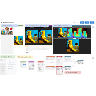
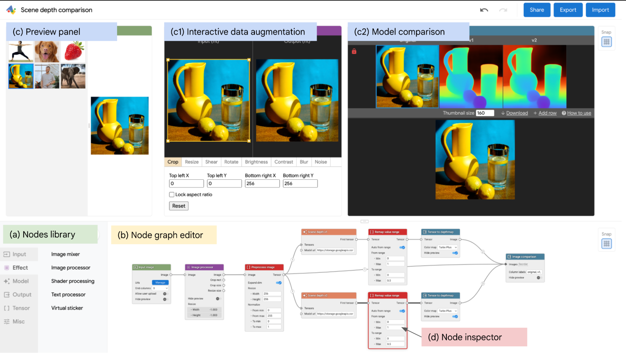
Visual Blocks is mainly written in JavaScript and leverages TensorFlow.js and TensorFlow Lite for ML capabilities and three.js for graphics rendering. The interface enables users to rapidly build and interact with ML models using three coordinated views: (1) a Nodes Library that contains over 30 nodes (e.g., Image Processing, Body Segmentation, Image Comparison) and a search bar for filtering, (2) a Node-graph Editor that allows users to build and adjust a multimedia pipeline by dragging and adding nodes from the Nodes Library, and (3) a Preview Panel that visualizes the pipeline’s input and output, alters the input and intermediate results, and visually compares different models.
 |
| The visual programming interface allows users to quickly develop and evaluate ML models by composing and previewing node-graphs with real-time results. |
Iterative design, development, and evaluation of unique rapid prototyping capabilities
Over the last year, we’ve been iteratively designing and improving the Visual Blocks platform. Weekly feedback sessions with the three ML teams from the formative study showed appreciation for the platform’s unique capabilities and its potential to accelerate ML prototyping through:
- Support for various types of input data (image, video, audio) and output modalities (graphics, sound).
- A library of pre-trained ML models for common tasks (body segmentation, landmark detection, portrait depth estimation) and custom model import options.
- Interactive data augmentation and manipulation with drag-and-drop operations and parameter sliders.
- Side-by-side comparison of multiple models and inspection of their outputs at different stages of the pipeline.
- Quick publishing and sharing of multimedia pipelines directly to the web.
Evaluation: Four case studies
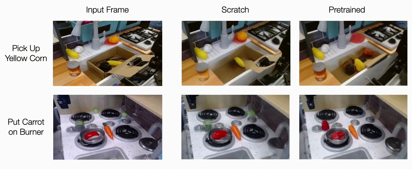
To evaluate the usability and effectiveness of Visual Blocks, we conducted four case studies with 15 ML practitioners. They used the platform to prototype different multimedia applications: portrait depth with relighting effects, scene depth with visual effects, alpha matting for virtual conferences, and audio denoising for communication.
 |
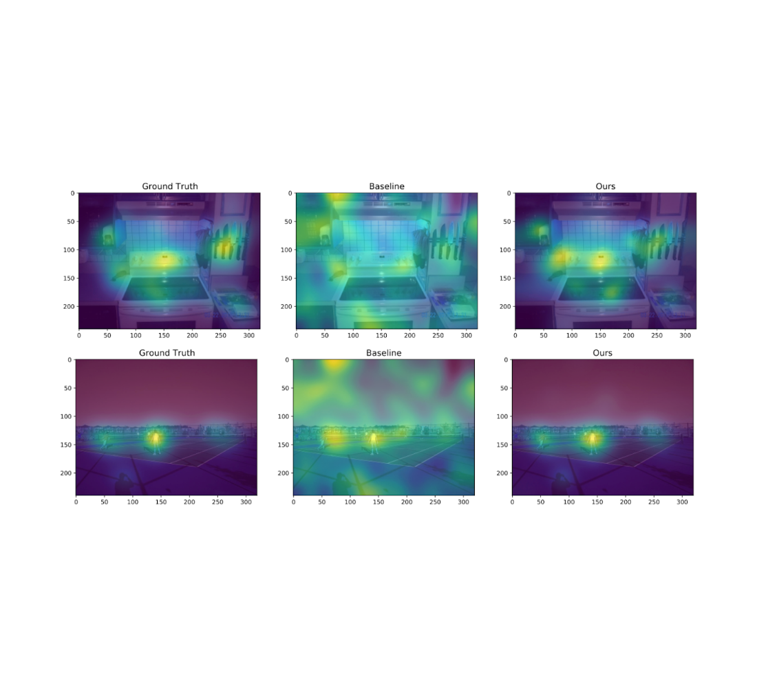
| The system streamlining comparison of two Portrait Depth models, including customized visualization and effects. |
With a short introduction and video tutorial, participants were able to quickly identify differences between the models and select a better model for their use case. We found that Visual Blocks helped facilitate rapid and deeper understanding of model benefits and trade-offs:
“It gives me intuition about which data augmentation operations that my model is more sensitive [to], then I can go back to my training pipeline, maybe increase the amount of data augmentation for those specific steps that are making my model more sensitive.” (Participant 13)
“It’s a fair amount of work to add some background noise, I have a script, but then every time I have to find that script and modify it. I’ve always done this in a one-off way. It’s simple but also very time consuming. This is very convenient.” (Participant 15)
 |
| The system allows researchers to compare multiple Portrait Depth models at different noise levels, helping ML practitioners identify the strengths and weaknesses of each. |
In a post-hoc survey using a seven-point Likert scale, participants reported Visual Blocks to be more transparent about how it arrives at its final results than Colab (Visual Blocks 6.13 ± 0.88 vs. Colab 5.0 ± 0.88, 𝑝 < .005) and more collaborative with users to come up with the outputs (Visual Blocks 5.73 ± 1.23 vs. Colab 4.15 ± 1.43, 𝑝 < .005). Although Colab assisted users in thinking through the task and controlling the pipeline more effectively through programming, Users reported that they were able to complete tasks in Visual Blocks in just a few minutes that could normally take up to an hour or more. For example, after watching a 4-minute tutorial video, all participants were able to build a custom pipeline in Visual Blocks from scratch within 15 minutes (10.72 ± 2.14). Participants usually spent less than five minutes (3.98 ± 1.95) getting the initial results, then were trying out different input and output for the pipeline.
 |
| User ratings between Rapsai (initial prototype of Visual Blocks) and Colab across five dimensions. |
More results in our paper showed that Visual Blocks helped participants accelerate their workflow, make more informed decisions about model selection and tuning, analyze strengths and weaknesses of different models, and holistically evaluate model behavior with real-world input.
Conclusions and future directions
Visual Blocks lowers development barriers for ML-based multimedia applications. It empowers users to experiment without worrying about coding or technical details. It also facilitates collaboration between designers and developers by providing a common language for describing ML pipelines. In the future, we plan to open this framework up for the community to contribute their own nodes and integrate it into many different platforms. We expect visual programming for machine learning to be a common interface across ML tooling going forward.
Acknowledgements
This work is a collaboration across multiple teams at Google. Key contributors to the project include Ruofei Du, Na Li, Jing Jin, Michelle Carney, Xiuxiu Yuan, Kristen Wright, Mark Sherwood, Jason Mayes, Lin Chen, Jun Jiang, Scott Miles, Maria Kleiner, Yinda Zhang, Anuva Kulkarni, Xingyu “Bruce” Liu, Ahmed Sabie, Sergio Escolano, Abhishek Kar, Ping Yu, Ram Iyengar, Adarsh Kowdle, and Alex Olwal.
We would like to extend our thanks to Jun Zhang and Satya Amarapalli for a few early-stage prototypes, and Sarah Heimlich for serving as a 20% program manager, Sean Fanello, Danhang Tang, Stephanie Debats, Walter Korman, Anne Menini, Joe Moran, Eric Turner, and Shahram Izadi for providing initial feedback for the manuscript and the blog post. We would also like to thank our CHI 2023 reviewers for their insightful feedback.

 Bard can now help with programming and software development tasks, across more than 20 programming languages.