This post is the fourth part of a multi-series blog focused on how to accelerate generative AI models with pure, native PyTorch. To skip to the code, check out our github (seamless_communication, fairseq2). We are excited to share a breadth of newly released PyTorch performance features alongside practical examples to see how far we can push PyTorch native performance. In part one, we showed how to accelerate Segment Anything over 8x using only pure, native PyTorch. In part two, we showed how to accelerate Llama-7B by almost 10x using only native PyTorch optimizations. In part three, we showed how to accelerate text-to-image diffusion models up to 3x using only native Pytorch optimizations.
In this blog, we’ll focus on speeding up FAIR’s Seamless M4T-v2 model resulting in 2x speedup for text decoder module and 30x for vocoder module, resulting in 2.7x speedup for end-to-end inference, with no loss of accuracy by using CUDA Graph and native PyTorch optimization:
Introduction
Seamless M4T is an open-source foundational speech/text translation and transcription technology developed by FAIR. Seamless M4T is a massively multilingual and multimodal machine translation model, with the latest version (Seamless M4T-v2) released on November 30th, 2023. The high-level model architecture of Seamless M4T-v2 is illustrated in Figure 1.
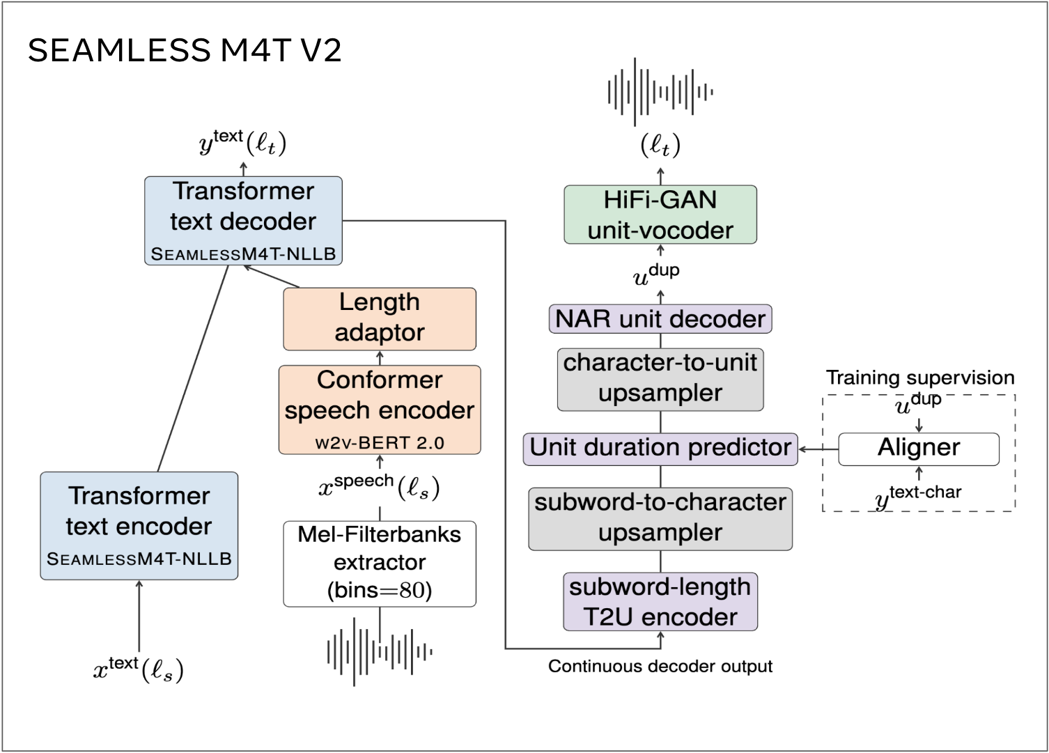
Figure 1. Model Architecture of Seamless M4T-v2.
Accelerating inference latency is crucial for translation models to improve user experience through faster communication across languages. In particular, batch_size=1 is often used for fast translation where latency matters a lot in applications such as chatbots, speech translation, and live subtitling. Therefore, we conducted the performance analysis on inference with batch_size=1, as shown in Figure 2 to understand the Amdahl’s Law bottleneck. Our results indicate that the text decoder and vocoder are the most time-consuming modules, accounting for 61% and 23% of the inference time, respectively.
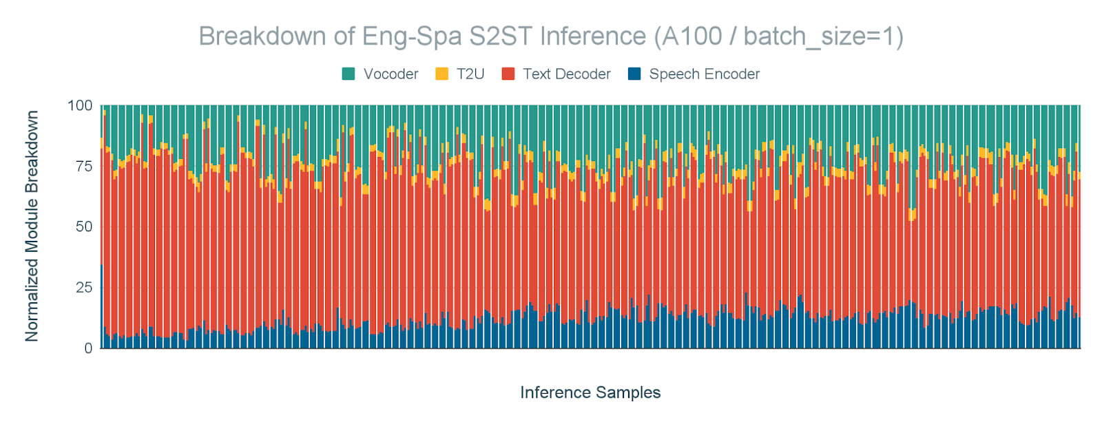
Figure 2. Text decoder and vocoder are the most time consuming module. Breakdown of inference time by modules for English-Spanish S2ST (Speech-to-Speech-Text) task for batch_size=1 on A100 GPU.
To take a closer look at the performance bottleneck of the text decoder and vocoder, we analyzed GPU traces for the text decoder and vocoder for the 8th sample for the English-Spanish translation example of FLEURS dataset as shown in Figure 3. It revealed that the text decoder and vocoder are heavily CPU-bound modules. We observed a significant gap incurred by CPU overhead that delayed the launch of GPU kernels, resulting in a substantial increase in the execution time for both the modules.
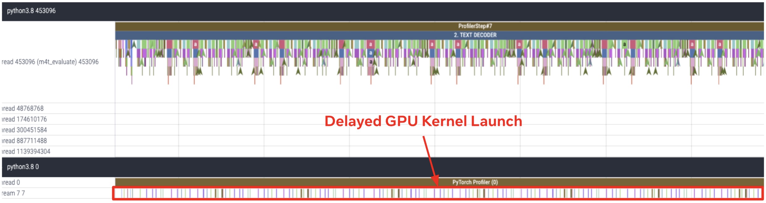
(a) CPU and GPU trace for Text Decoder
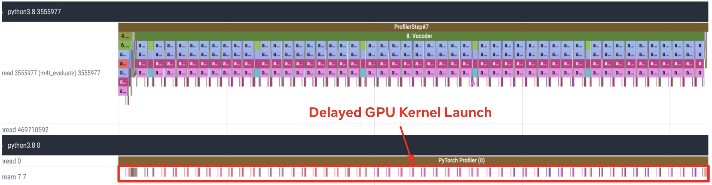
(b) CPU and GPU trace for Vocoder
Figure 3. Text Decoder and Vocoder are heavily CPU-bound modules. CPU and GPU trace for (a) Text Decoder (b) Vocoder for the 8th sample for English-Spanish translation example of FLEURS dataset. The trace is obtained by running inference with batch_size=1 on A100 gpu.
Based on the real-system performance analysis results that text_decoder and vocoder are heavily CPU bound modules in Seamless M4T-v2, we enabled torch.compile + CUDA Graph to those modules. In this post, we share modifications required to enable torch.compile + CUDA Graph on each module for batch_size=1 inference scenario, discussion on CUDA Graph and next step plans.
Torch.compile with CUDA Graph
torch.compile is a PyTorch API that allows users to compile PyTorch models into a standalone executable or script which is generally used for optimizing model performance by removing unnecessary overhead.
CUDA Graph is a feature provided by NVIDIA that allows for the optimization of kernel launches in CUDA applications. It creates an execution graph of CUDA kernels, which can be pre-processed and optimized by the driver before being executed on the GPU. The main advantage of using CUDA Graph is that it reduces the overhead associated with launching individual kernels, as the graph can be launched as a single unit, reducing the number of API calls and data transfers between the host and device. This can lead to significant performance improvements, especially for applications that have a large number of small kernels or repeat the same set of kernels multiple times. If this is something you are interested in learning more about, check out this paper that highlights the important role of data for accelerated computing: Where is the data? Why you cannot debate CPU vs. GPU performance without the answer by our own Kim Hazelwood! This is when NVIDIA was heavily investing in general-purpose GPU (GPGPUs) and before deep learning revolutionized the computing industry!
However, because CUDA Graph operates on 1) fixed memory pointer, 2) fixed shape of tensors, that are recorded at the compile time, we introduced the following improvements for CUDA Graph to be reused across multiple sizes of inputs to prevent CUDA Graph generation for each iteration and let the data inside CUDA Graph be reused across different runs to share KV Cache for multiple decoding steps.
Text Decoder
The Text Decoder in Seamless is a decoder from NLLB [1] that performs T2TT (Text to Text Translation). Also, this module is a CPU-bound model where gpu execution time is not long enough to hide CPU overhead because of the nature of auto-regressive generation that requires sequential processing of tokens, which limits the amount of parallelism that can be achieved on the GPU. Based on this observation, we enabled torch.compile + CUDA Graph for the text decoders to reduce the dominating CPU overhead as shown in Figure 4.
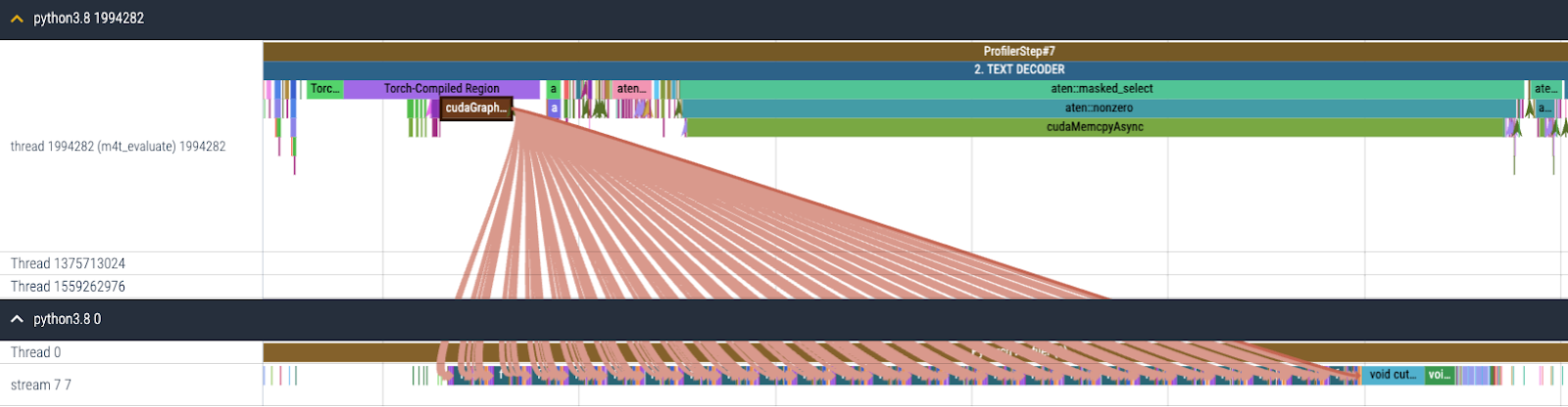
Figure 4. CPU and GPU trace for Text Decoder after torch.compile + CUDA Graph are enabled.
1. Updating and retrieving KV cache
During inference, the text decoder has two computation phases: a prefill phase that consumes the prompt and an incremental generation phase that generates output tokens one by one. Given a high enough batch size or input length, prefill operates on a sufficiently high number of tokens in parallel — GPU performance is the bottleneck and the CPU overheads do not impact performance significantly. On the other hand, incremental token generation is always executed with sequence length 1 and it is often executed with a small batch size (even 1), e.g. for interactive use cases. Thus, incremental generation can be limited by the CPU speed and thus is a good candidate for torch.compile + CUDA Graph.
However, during the incremental token generation phase, the sequence_length dimension of key and value involved in the attention computation increases by one with each step while the sequence length of query always remains 1. Specifically, key/value are generated by appending the newly computed key/value of sequence length 1 to the key/value stored in the KV cache so far. But as mentioned above, CUDA Graph records all the shapes of tensors during compilation and replay with the recorded shapes. Thus, few modifications have been made to address this issue following the great work here.
a) We modify the KV-cache handling to take the indices in which to write new values in a CUDA Tensor (i.e., valid_seq_pos) rather than a Python integer.
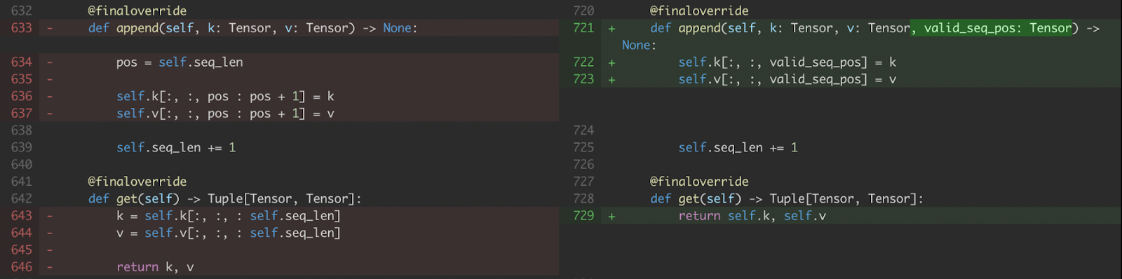
Figure 5. Modification to KV cache append and get
b) We also modify attention to work with the fixed shape of key and value over the max_seq_length. We only compute softmax over the sequence positions up to the current decoding step (i.e., valid_seq_pos) . To mask out sequence positions > current decoding step (i.e., valid_seq_pos), we create a boolean mask tensor (i.e., mask) where sequence positions > valid_seq_pos are set to False.
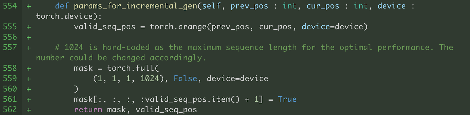
Figure 6. Helper function to generate valid_seq_pos and mask
It’s important to post that these modifications result in an increase in the amount of computation required, as we compute attention over more sequence positions than necessary (up to max_seq_length). However, despite this drawback, our results demonstrate that torch.compile + CUDA Graph still provide significant performance benefits compared to standard PyTorch code.
c) As different inference samples have different sequence length, it also generates different shapes of inputs that are to be projected to key and value for the cross attention layers. Thus, we pad the input to have a static shape and generate a padding mask to mask out padded output.
2. Memory Pointer Management
As CUDA Graph records memory pointers along with the shape of tensors, it is important to make different inference samples to correctly reference the recorded memory pointer (e.g., KV cache) to avoid compiling CUDA Graph for each inference sample. However, some parts of the Seamless codebase made different inference samples to refer to different memory addresses, so we made modifications to improve the memory implications.
e) Seamless adopts beam search as a text decoding strategy. In the beam search process, we need to perform KV cache reordering for all the attention layers for each incremental decoding step to make sure each selected beam performs with corresponding KV cache as shown in the code snippet below.
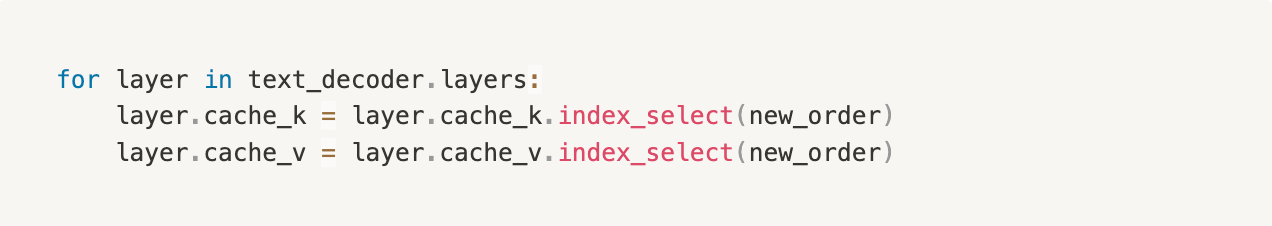
Figure 8. KV cache reordering operation for beam search decoding strategy.
The above code allocates new memory space and overwrites the original memory pointer for cache_k and cache_v. Thus we modified KV cache reordering to keep the memory pointer of each cache as was recorded during compilation by using copy_ operator.
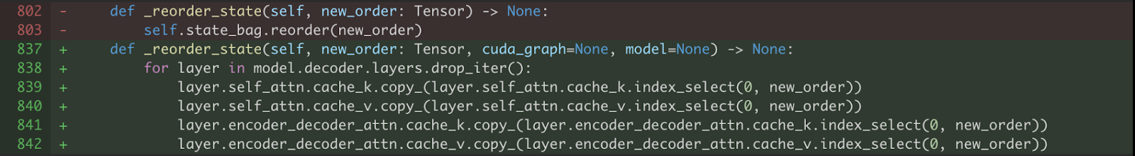
Figure 9. In-place update for KV cache using copy_ operator
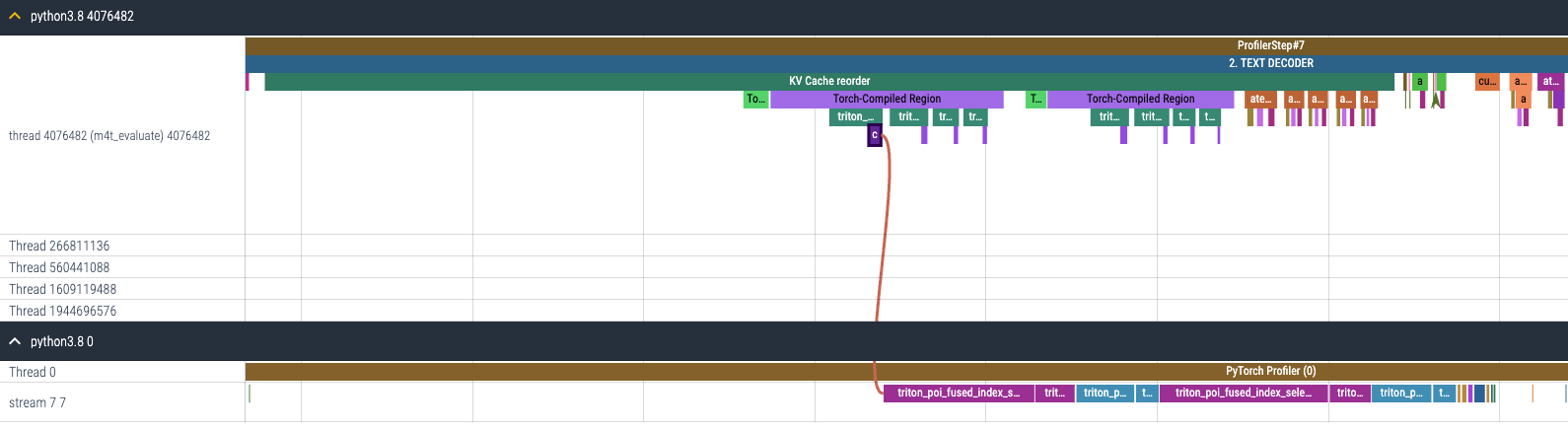
f) After enabling torch.compile + CUDA Graph to text decoder by modifying the code as mentioned above, the overhead of text decoder shifts to KV cache reordering as shown in Figure 10. KV cache reordering repeatedly calls index_select 96 times (assuming 24 decoder layers where each layer consists of two types of attention layers with cache for key and value).
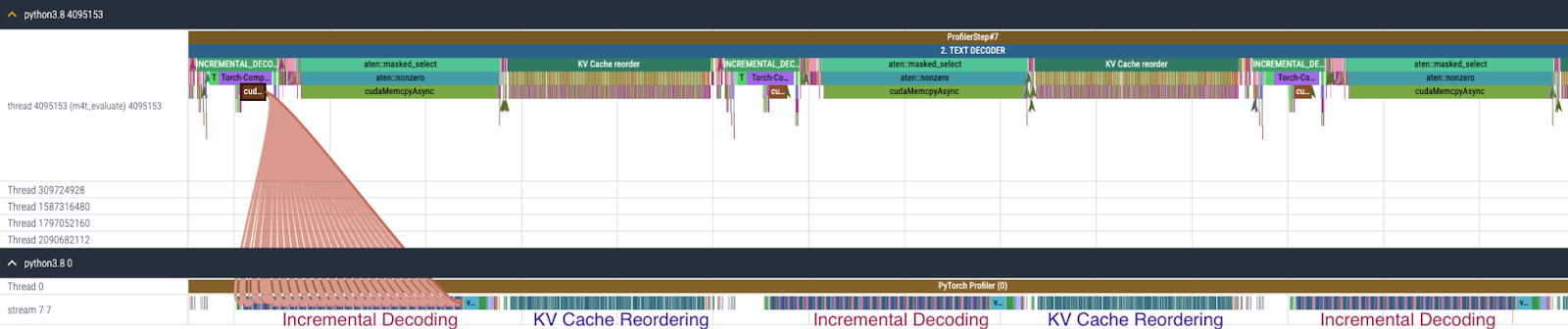
Figure 10. CPU and GPU trace for Text Decoder after enabling torch.compile + CUDA Graph.
As part of accelerating text decoder, we additionally applied torch.compile to KV cache reordering to benefit from fusing kernels as shown in Figure 11. Note that we cannot use CUDA Graph here (mode='max-autotune') here, because copy_ operation modifies the inputs which violates the static input requirement of CUDA graph version in torch.compile.
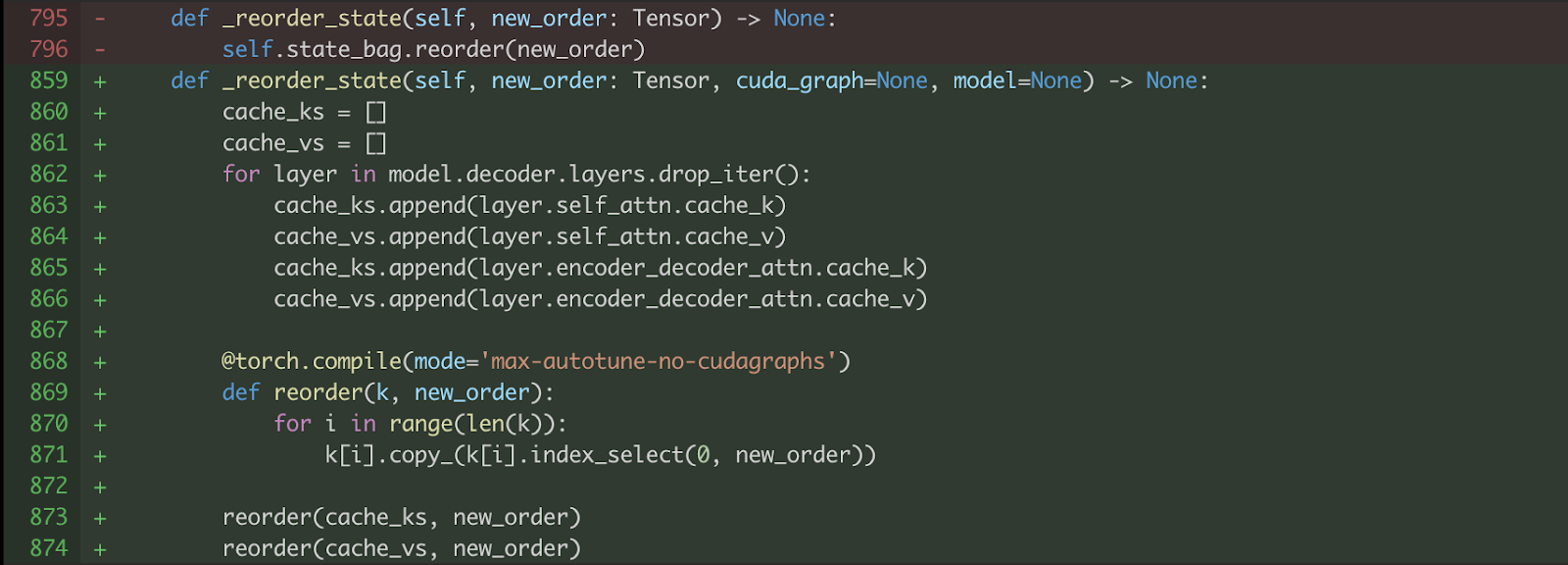
Figure 11. Applying torch.compile to KV Cache reordering.
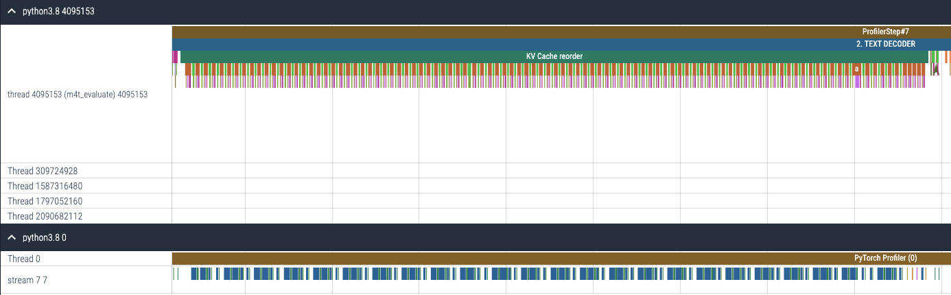
As a result of enabling torch.compile to KV cache reordering, the gpu kernels that were launched separately (Figure 12(a)) are now fused so there are much fewer gpu kernels to launch (Figure 12(b)).
(a) CPU and GPU trace for KV cache reordering before enabling torch.compile
(b) CPU and GPU trace for KV cache reordering after enabling torch.compile
Figure 12. CPU and GPU trace for KV cache reordering (a) before and (b) after enabling torch.compile
Vocoder
Vocoder in Seamless is a HiFi-GAN unit-vocoder that converts generated units to waveform output where an unit is a representation of speech that combines different aspects such as phonemes and syllables, which can be used to generate sounds that are audible to humans. Vocoder is a relatively simple module that consists of Conv1d and ConvTranspose1d layers and is a CPU bound module as shown in FIgure 3. Based on this observation, we decided to enable torch.compile + CUDA Graph for vocoder to reduce the disproportionally large CPU overhead as shown in Figure 10. But there were several fixes to be made.
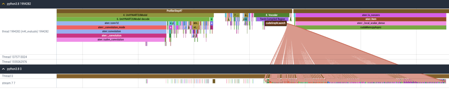
Figure 13. CPU and GPU trace for Vocoder after torch.compile + CUDA Graph are enabled.
a) The input tensor shape of the vocoder is different across different inference samples. But as CUDA Graph records the shape of tensors and replays them, we had to pad the input to the fixed size with zeros. Since vocoder only consists of Conv1d layers, we do not need an additional padding mask, and padding with zeros is sufficient.
b) Vocoder consists of conv1d layers wrapped with torch.nn.utils.weight_norm (see here). However, applying torch.compile directly to Vocoder incurs graph break as below, which leads to suboptimal performance improvement. This graph break happens inside the hook handling part in the PyTorch code of weight_norm.
[1/0_2] torch._dynamo.symbolic_convert.__graph_breaks: [DEBUG] Graph break: setattr(UserDefinedObjectVariable) <function Module.__setattr__ at 0x7fac8f483c10> from user code at:
[1/0_2] torch._dynamo.symbolic_convert.__graph_breaks: [DEBUG]   File "/mnt/fsx-home/yejinlee/yejinlee/seamless_communication/src/seamless_communication/models/vocoder/vocoder.py", line 49, in forward
[1/0_2] torch._dynamo.symbolic_convert.__graph_breaks: [DEBUG]     return self.code_generator(x, dur_prediction)  # type: ignore[no-any-return]1/0_2] torch._dynamo.symbolic_convert.__graph_breaks: [DEBUG]   File "/data/home/yejinlee/mambaforge/envs/fairseq2_12.1/lib/python3.8/site-packages/torch/nn/modules/module.py", line 1520, in _call_impl
[1/0_2] torch._dynamo.symbolic_convert.__graph_breaks: [DEBUG]     return forward_call(*args, **kwargs)
[2023-12-13 04:26:16,822] [1/0_2] torch._dynamo.symbolic_convert.__graph_breaks: [DEBUG]   File "/mnt/fsx-home/yejinlee/yejinlee/seamless_communication/src/seamless_communication/models/vocoder/codehifigan.py", line 101, in forward
[1/0_2] torch._dynamo.symbolic_convert.__graph_breaks: [DEBUG]     return super().forward(x)
[1/0_2] torch._dynamo.symbolic_convert.__graph_breaks: [DEBUG]   File "/mnt/fsx-home/yejinlee/yejinlee/seamless_communication/src/seamless_communication/models/vocoder/hifigan.py", line 185, in forward
[1/0_2] torch._dynamo.symbolic_convert.__graph_breaks: [DEBUG]     x = self.ups[i](x)
[1/0_2] torch._dynamo.symbolic_convert.__graph_breaks: [DEBUG]   File "/data/home/yejinlee/mambaforge/envs/fairseq2_12.1/lib/python3.8/site-packages/torch/nn/modules/module.py", line 1550, in _call_impl
[1/0_2] torch._dynamo.symbolic_convert.__graph_breaks: [DEBUG]     args_result = hook(self, args)
[1/0_2] torch._dynamo.symbolic_convert.__graph_breaks: [DEBUG]   File "/data/home/yejinlee/mambaforge/envs/fairseq2_12.1/lib/python3.8/site-packages/torch/nn/utils/weight_norm.py", line 65, in __call__
[1/0_2] torch._dynamo.symbolic_convert.__graph_breaks: [DEBUG]     setattr(module, self.name, self.compute_weight(module))
[1/0_2] torch._dynamo.symbolic_convert.__graph_breaks: [DEBUG]
Since the weights of layers do not change during the inference, we do not need weight normalization. So we simply removed weight normalization for Vocoder as shown in Figure 14, by utilizing remove_weight_norm function which is already provided at the Seamless codebase (here).
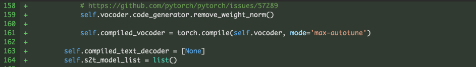
Figure 14. Removing weight_norm for Vocoder
Performance Evaluation + Impact of CUDA Graph
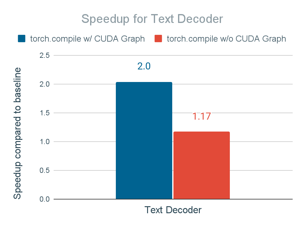
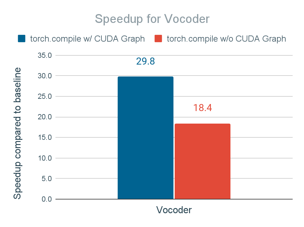
Figure 15 shows the speedup result when enabling torch.compile(mode=”max-autotune”) + CUDA Graph on the text decoder and vocoder. We achieve 2x speedup for the text decoder and 30x speedup for vocoder, leading to 2.7x faster end-to-end inference time.
Figure 15. Inference time speedup of text decoder and vocoder of applying torch.compile and torch.compile + CUDA Graph
We also report the speedups for text decoder and vocoder using torch.compile without CUDA Graph, which is supported by torch.compile’s API (i.e., torch.compile(mode="max-autotune-no-cudagraphs")), to identify the impact of CUDA Graph on the performance. Without CUDA Graph, the speedup for text decoder and vocoder reduces to 1.17x and 18.4x. While still quite significant, it indicates the important role of CUDA Graph. We conclude that Seamless M4T-v2 is exposed to a lot of time launching CUDA kernels, especially when we use small batch size (e.g., 1) where the GPU kernel execution time is not long enough to amortize the GPU kernel launch time.
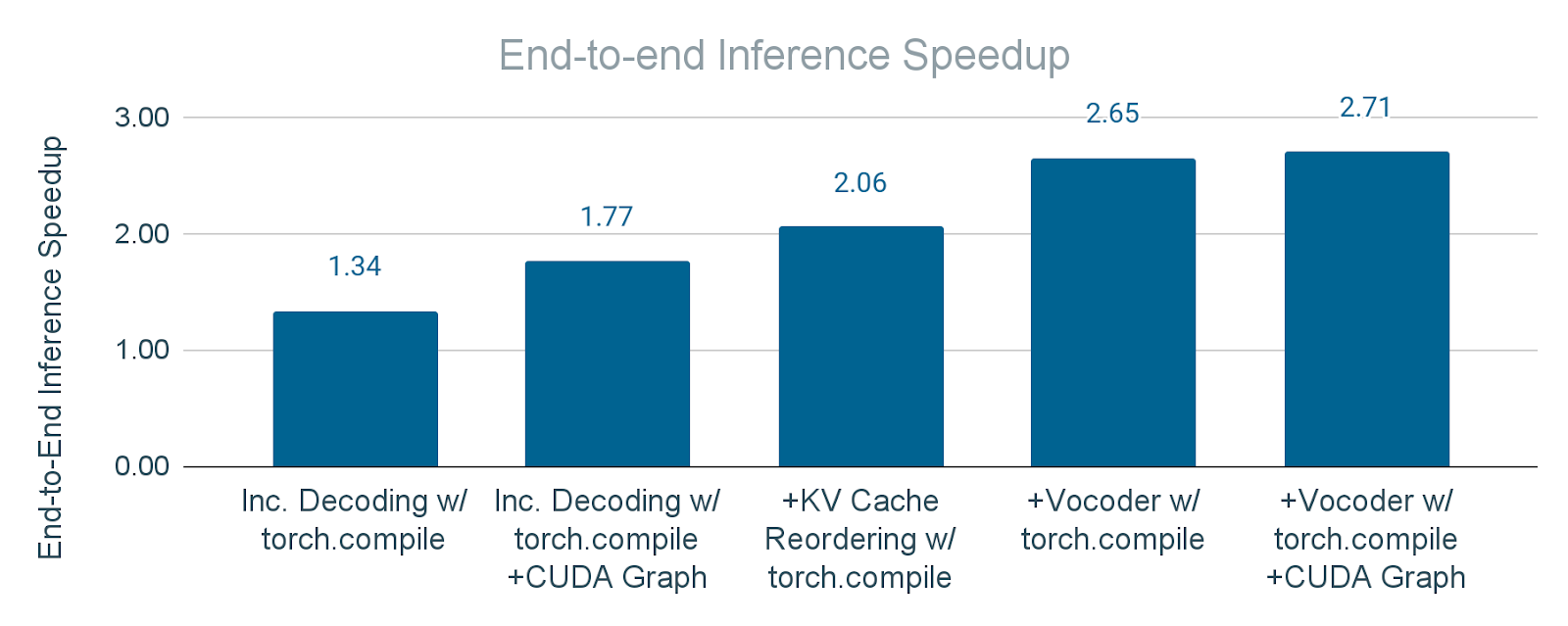
Figure 16. End-to-end inference speedup of applying torch.compile and CUDA graph incrementally. a) “Inc. Decoding”: Apply torch.compile only to the text decoder b) “Inc. Decoding w/ CUDA Graph”: Apply torch.compile + CUDA Graph to the text decoder c) “+KV Cache Reordering”: Additionally apply torch.compile to KV cache reordering operation upon b) d) “+Vocoder”: Additionally apply torch.compile to the vocoder upon c) e) “+Vocoder w/ CUDA Graph”: Additionally apply torch.compile + CUDA Graph to the vocoder upon d).
Figure 16 represents the cumulative effect of applying torch.compile with and without CUDA Graph to the modules. The results indicate a significant improvement in the end-to-end inference speedup, demonstrating the effectiveness of these techniques in optimizing the overall latency. As a result, we gain 2.7x end-to-end inference speedup for Seamless M4T-v2 with batch_size=1.
Acknowledgements
We thank the PyTorch team and Seamless team for their tremendous support with this work.
Read More