TorchGeo is a PyTorch domain library providing datasets, samplers, transforms, and pre-trained models specific to geospatial data.

https://github.com/microsoft/torchgeo

For decades, Earth observation satellites, aircraft, and more recently UAV platforms have been collecting increasing amounts of imagery of the Earth’s surface. With information about seasonal and long-term trends, remotely sensed imagery can be invaluable for solving some of the greatest challenges to humanity, including climate change adaptation, natural disaster monitoring, water resource management, and food security for a growing global population. From a computer vision perspective, this includes applications like land cover mapping (semantic segmentation), deforestation and flood monitoring (change detection), glacial flow (pixel tracking), hurricane tracking and intensity estimation (regression), and building and road detection (object detection, instance segmentation). By leveraging recent advancements in deep learning architectures, cheaper and more powerful GPUs, and petabytes of freely available satellite imagery datasets, we can come closer to solving these important problems.

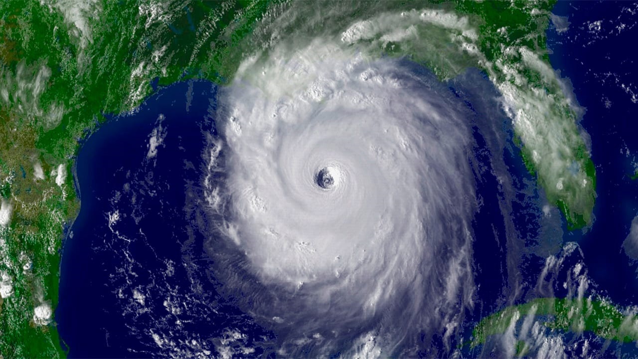
National Oceanic and Atmospheric Administration satellite image of Hurricane Katrina, taken on August 28, 2005 (source). Geospatial machine learning libraries like TorchGeo can be used to detect, track, and predict future trajectories of hurricanes and other natural disasters.

The challenges

In traditional computer vision datasets, such as ImageNet, the image files themselves tend to be rather simple and easy to work with. Most images have 3 spectral bands (RGB), are stored in common file formats like PNG or JPEG, and can be easily loaded with popular software libraries like PIL or OpenCV. Each image in these datasets is usually small enough to pass directly into a neural network. Furthermore, most of these datasets contain a finite number of well-curated images that are assumed to be independent and identically distributed, making train-val-test splits straightforward. As a result of this relative homogeneity, the same pre-trained models (e.g., CNNs pretrained on ImageNet) have shown to be effective across a wide range of vision tasks using transfer learning methods. Existing libraries, such as torchvision, handle these simple cases well, and have been used to make large advances in vision tasks over the past decade.

Remote sensing imagery is not so uniform. Instead of simple RGB images, satellites tend to capture images that are multispectral (Landsat 8 has 11 spectral bands) or even hyperspectral (Hyperion has 242 spectral bands). These images capture information at a wider range of wavelengths (400 nm–15 µm), far outside of the visible spectrum. Different satellites also have very different spatial resolutions—GOES has a resolution of 4 km/px, Maxar imagery is 30 cm/px, and drone imagery resolution can be as high as 7 mm/px. These datasets almost always have a temporal component, with satellite revisists that are daily, weekly, or biweekly. Images often have overlap with other images in the dataset, and need to be stitched together based on geographic metadata. These images tend to be very large (e.g., 10K x 10K pixels), so it isn’t possible to pass an entire image through a neural network. This data is distributed in hundreds of different raster and vector file formats like GeoTIFF and ESRI Shapefile, requiring specialty libraries like GDAL to load.

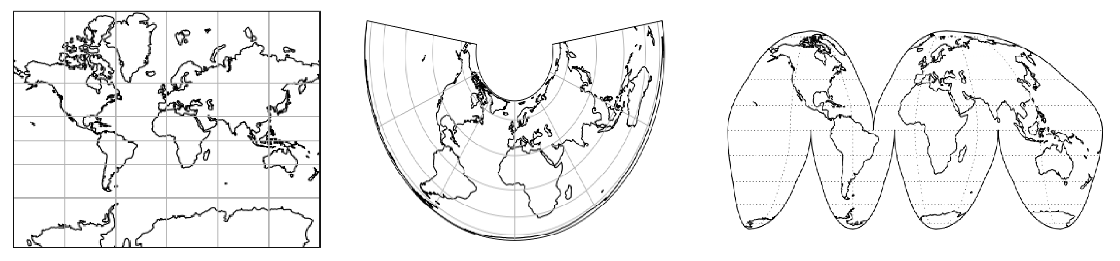
From left to right: Mercator, Albers Equal Area, and Interrupted Goode Homolosine projections (source). Geospatial data is associated with one of many different types of reference systems that project the 3D Earth onto a 2D representation. Combining data from different sources often involves re-projecting to a common reference system in order to ensure that all layers are aligned.

Although each image is 2D, the Earth itself is 3D. In order to stitch together images, they first need to be projected onto a 2D representation of the Earth, called a coordinate reference system (CRS). Most people are familiar with equal angle representations like Mercator that distort the size of regions (Greenland looks larger than Africa even though Africa is 15x larger), but there are many other CRSs that are commonly used. Each dataset may use a different CRS, and each image within a single dataset may also be in a unique CRS. In order to use data from multiple layers, they must all share a common CRS, otherwise the data won’t be properly aligned. For those who aren’t familiar with remote sensing data, this can be a daunting task.

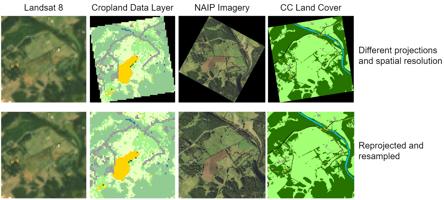
Even if you correctly georeference images during indexing, if you don’t project them to a common CRS, you’ll end up with rotated images with nodata values around them, and the images won’t be pixel-aligned.

The solution

At the moment, it can be quite challenging to work with both deep learning models and geospatial data without having expertise in both of these very different fields. To address these challenges, we’ve built TorchGeo, a PyTorch domain library for working with geospatial data. TorchGeo is designed to make it simple:

1. for machine learning experts to work with geospatial data, and
2. for remote sensing experts to explore machine learning solutions.

TorchGeo is not just a research project, but a production-quality library that uses continuous integration to test every commit with a range of Python versions on a range of platforms (Linux, macOS, Windows). It can be easily installed with any of your favorite package managers, including pip, conda, and spack:

$ pip install torchgeo

TorchGeo is designed to have the same API as other PyTorch domain libraries like torchvision, torchtext, and torchaudio. If you already use torchvision in your workflow for computer vision datasets, you can switch to TorchGeo by changing only a few lines of code. All TorchGeo datasets and samplers are compatible with the PyTorch DataLoader class, meaning that you can take advantage of wrapper libraries like PyTorch Lightning for distributed training. In the following sections, we’ll explore possible use cases for TorchGeo to show how simple it is to use.

Geospatial datasets and samplers

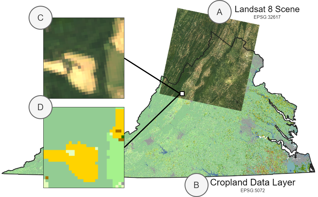
Example application in which we combine A) a scene from Landsat 8 and B) Cropland Data Layer labels, even though these files are in different EPSG projections. We want to sample patches C) and D) from these datasets using a geospatial bounding box as an index.

Many remote sensing applications involve working with geospatial datasets —datasets with geographic metadata. In TorchGeo, we define a GeoDataset class to represent these kinds of datasets. Instead of being indexed by an integer, each GeoDataset is indexed by a spatiotemporal bounding box, meaning that two or more datasets covering a different geographic extent can be intelligently combined.

In this example, we show how easy it is to work with geospatial data and to sample small image patches from a combination of Landsat and Cropland Data Layer (CDL) data using TorchGeo. First, we assume that the user has Landsat 7 and 8 imagery downloaded. Since Landsat 8 has more spectral bands than Landsat 7, we’ll only use the bands that both satellites have in common. We’ll create a single dataset including all images from both Landsat 7 and 8 data by taking the union between these two datasets.

from torch.utils.data import DataLoader
from torchgeo.datasets import CDL, Landsat7, Landsat8, stack_samples
from torchgeo.samplers import RandomGeoSampler

landsat7 = Landsat7(root="...")
landsat8 = Landsat8(root="...", bands=Landsat8.all_bands[1:-2])
landsat = landsat7 | landsat8

Next, we take the intersection between this dataset and the CDL dataset. We want to take the intersection instead of the union to ensure that we only sample from regions where we have both Landsat and CDL data. Note that we can automatically download and checksum CDL data. Also note that each of these datasets may contain files in different CRSs or resolutions, but TorchGeo automatically ensures that a matching CRS and resolution is used.

cdl = CDL(root="...", download=True, checksum=True)
dataset = landsat & cdl

This dataset can now be used with a PyTorch data loader. Unlike benchmark datasets, geospatial datasets often include very large images. For example, the CDL dataset consists of a single image covering the entire contiguous United States. In order to sample from these datasets using geospatial coordinates, TorchGeo defines a number of samplers. In this example, we’ll use a random sampler that returns 256 x 256 pixel images and 10,000 samples per epoch. We’ll also use a custom collation function to combine each sample dictionary into a mini-batch of samples.

sampler = RandomGeoSampler(dataset, size=256, length=10000)
dataloader = DataLoader(dataset, batch_size=128, sampler=sampler, collate_fn=stack_samples)

This data loader can now be used in your normal training/evaluation pipeline.

for batch in dataloader:
    image = batch["image"]
    mask = batch["mask"]

    # train a model, or make predictions using a pre-trained model

Many applications involve intelligently composing datasets based on geospatial metadata like this. For example, users may want to:

• Combine datasets for multiple image sources and treat them as equivalent (e.g., Landsat 7 and 8)
• Combine datasets for disparate geospatial locations (e.g., Chesapeake NY and PA)

These combinations require that all queries are present in at least one dataset, and can be created using a UnionDataset. Similarly, users may want to:

• Combine image and target labels and sample from both simultaneously (e.g., Landsat and CDL)
• Combine datasets for multiple image sources for multimodal learning or data fusion (e.g., Landsat and Sentinel)

These combinations require that all queries are present in both datasets, and can be created using an IntersectionDataset. TorchGeo automatically composes these datasets for you when you use the intersection (&) and union (|) operators.

Multispectral and geospatial transforms

In deep learning, it’s common to augment and transform the data so that models are robust to variations in the input space. Geospatial data can have variations such as seasonal changes and warping effects, as well as image processing and capture issues like cloud cover and atmospheric distortion. TorchGeo utilizes augmentations and transforms from the Kornia library, which supports GPU acceleration and supports multispectral imagery with more than 3 channels.

Traditional geospatial analyses compute and visualize spectral indices which are combinations of multispectral bands. Spectral indices are designed to highlight areas of interest in a multispectral image relevant to some application, such as vegetation health, areas of man-made change or increasing urbanization, or snow cover. TorchGeo supports numerous transforms, which can compute common spectral indices and append them as additional bands to a multispectral image tensor.

Below, we show a simple example where we compute the Normalized Difference Vegetation Index (NDVI) on a Sentinel-2 image. NDVI measures the presence of vegetation and vegetation health and is computed as the normalized difference between the red and near-infrared (NIR) spectral bands. Spectral index transforms operate on sample dictionaries returned from TorchGeo datasets and append the resulting spectral index to the image channel dimension.

First, we instantiate a Sentinel-2 dataset and load a sample image. Then, we plot the true color (RGB) representation of this data to see the region we are looking at.

import matplotlib.pyplot as plt
from torchgeo.datasets import Sentinel2
from torchgeo.transforms import AppendNDVI

dataset = Sentinel2(root="...")
sample = dataset[...]
fig = dataset.plot(sample)
plt.show()

Next, we instantiate and compute an NDVI transform, appending this new channel to the end of the image. Sentinel-2 imagery uses index 0 for its red band and index 3 for its NIR band. In order to visualize the data, we also normalize the image. NDVI values can range from -1 to 1, but we want to use the range 0 to 1 for plotting.

transform = AppendNDVI(index_red=0, index_nir=3)
sample = transform(sample)
sample["image"][-1] = (sample["image"][-1] + 1) / 2
plt.imshow(sample["image"][-1], cmap="RdYlGn_r")
plt.show()

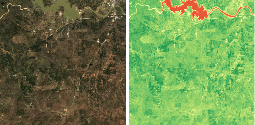
True color (left) and NDVI (right) of the Texas Hill Region, taken on November 16, 2018 by the Sentinel-2 satellite. In the NDVI image, red indicates water bodies, yellow indicates barren soil, light green indicates unhealthy vegetation, and dark green indicates healthy vegetation.

Benchmark datasets

One of the driving factors behind progress in computer vision is the existence of standardized benchmark datasets like ImageNet and MNIST. Using these datasets, researchers can directly compare the performance of different models and training procedures to determine which perform the best. In the remote sensing domain, there are many such datasets, but due to the aforementioned difficulties of working with this data and the lack of existing libraries for loading these datasets, many researchers opt to use their own custom datasets.

One of the goals of TorchGeo is to provide easy-to-use data loaders for these existing datasets. TorchGeo includes a number of benchmark datasets —datasets that include both input images and target labels. This includes datasets for tasks like image classification, regression, semantic segmentation, object detection, instance segmentation, change detection, and more.

If you’ve used torchvision before, these types of datasets should be familiar. In this example, we’ll create a dataset for the Northwestern Polytechnical University (NWPU) very-high-resolution ten-class (VHR-10) geospatial object detection dataset. This dataset can be automatically downloaded, checksummed, and extracted, just like with torchvision.

from torch.utils.data import DataLoader
from torchgeo.datasets import VHR10

dataset = VHR10(root="...", download=True, checksum=True)
dataloader = DataLoader(dataset, batch_size=128, shuffle=True, num_workers=4)

for batch in dataloader:
    image = batch["image"]
    label = batch["label"]

    # train a model, or make predictions using a pre-trained model

All TorchGeo datasets are compatible with PyTorch data loaders, making them easy to integrate into existing training workflows. The only difference between a benchmark dataset in TorchGeo and a similar dataset in torchvision is that each dataset returns a dictionary with keys for each PyTorch Tensor.

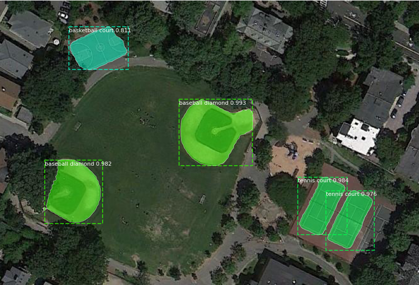
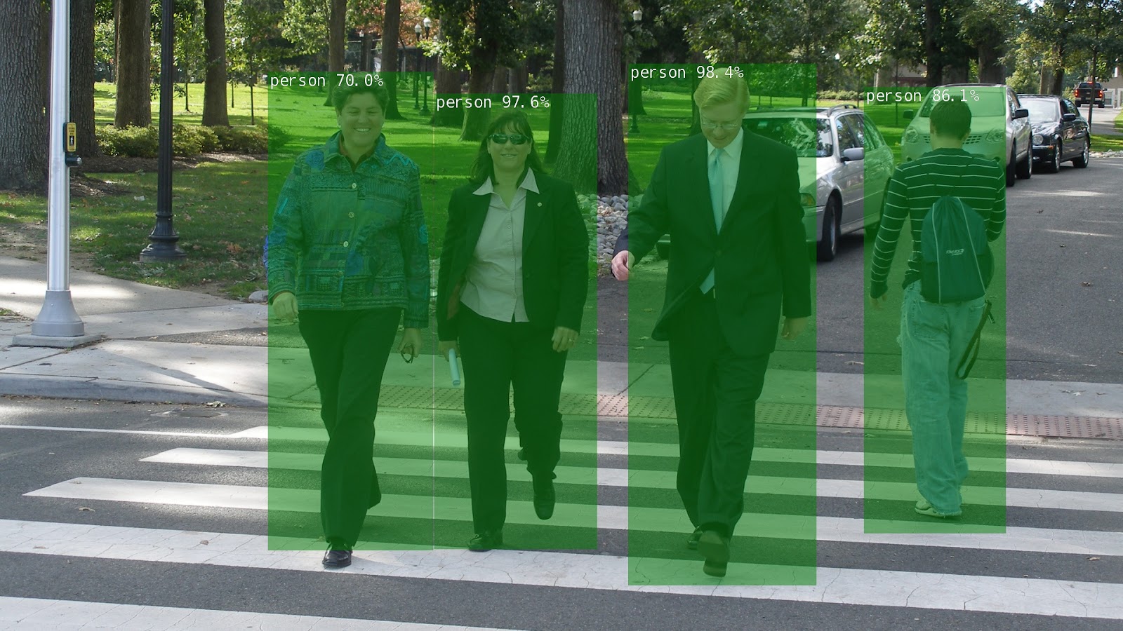
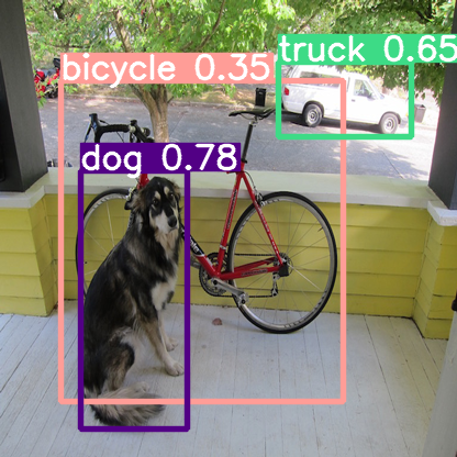
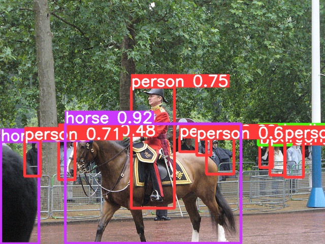
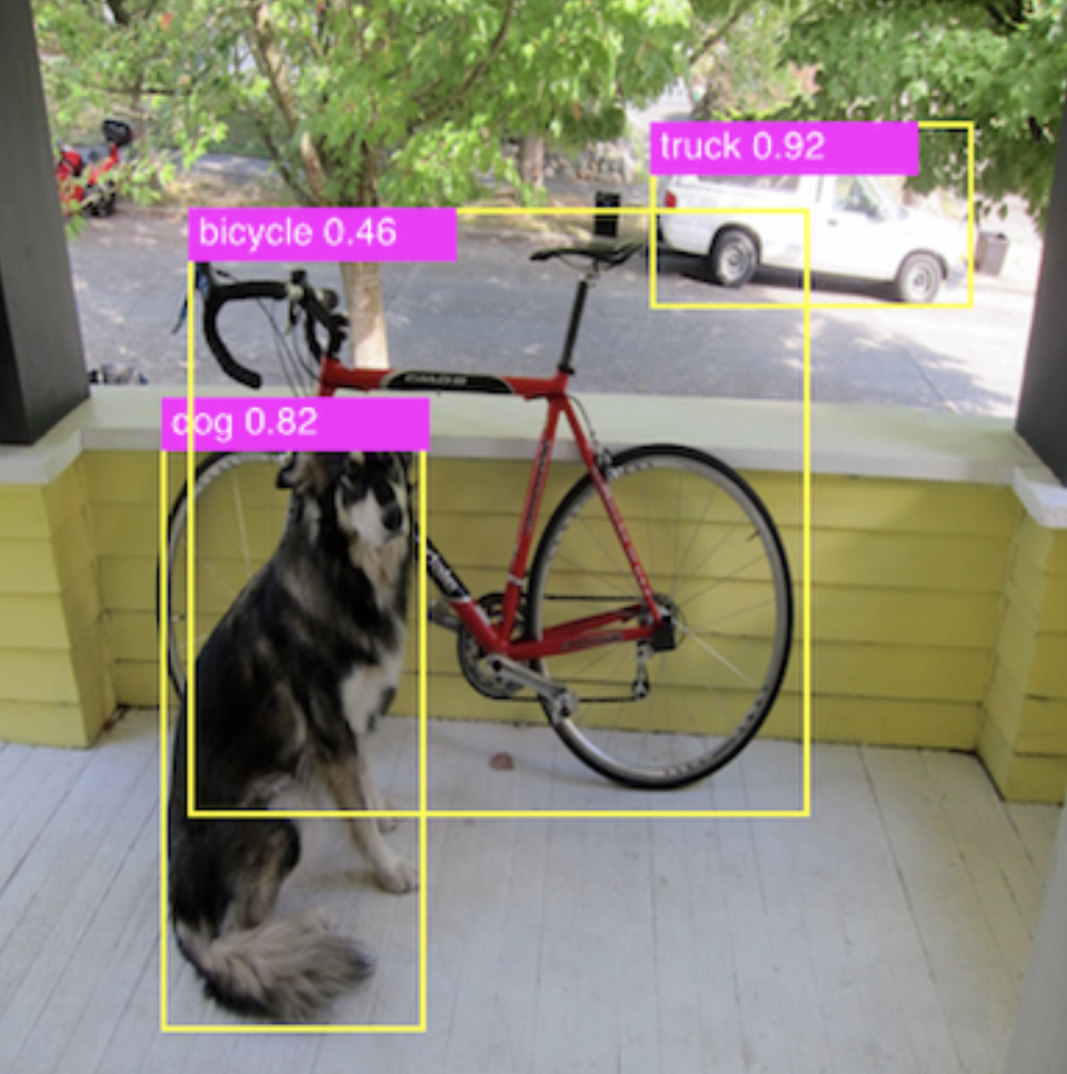
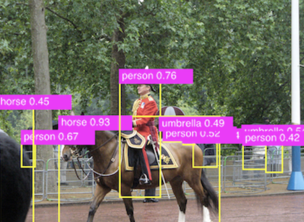
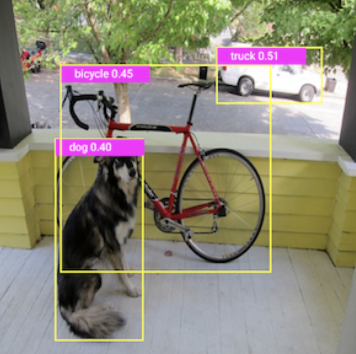
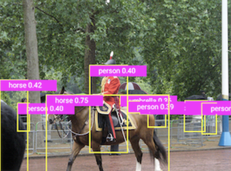
Example predictions from a Mask R-CNN model trained on the NWPU VHR-10 dataset. The model predicts sharp bounding boxes and masks for all objects with high confidence scores.

Reproducibility with PyTorch Lightning

Another key goal of TorchGeo is reproducibility. For many of these benchmark datasets, there is no predefined train-val-test split, or the predefined split has issues with class imbalance or geographic distribution. As a result, the performance metrics reported in the literature either can’t be reproduced, or aren’t indicative of how well a pre-trained model would work in a different geographic location.

In order to facilitate direct comparisons between results published in the literature and further reduce the boilerplate code needed to run experiments with datasets in TorchGeo, we have created PyTorch Lightning datamodules with well-defined train-val-test splits and trainers for various tasks like classification, regression, and semantic segmentation. These datamodules show how to incorporate augmentations from the kornia library, include preprocessing transforms (with pre-calculated channel statistics), and let users easily experiment with hyperparameters related to the data itself (as opposed to the modeling process). Training a regression model on the Inria Aerial Image Labeling dataset is as easy as a few imports and four lines of code.

from pytorch_lightning import Trainer
from torchgeo.datamodules import InriaAerialImageLabelingDataModule
from torchgeo.trainers import SemanticSegmentationTask

datamodule = InriaAerialImageLabelingDataModule(root_dir="...", batch_size=64, num_workers=6)
task = SemanticSegmentationTask(model="resnet18", pretrained=True, learning_rate=0.1)
trainer = Trainer(gpus=1, default_root_dir="...")

trainer.fit(model=task, datamodule=datamodule)

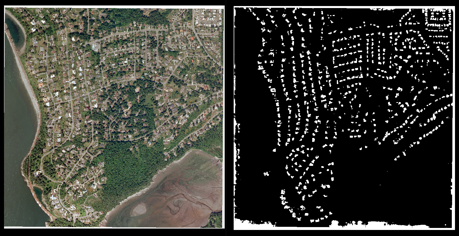
Building segmentations produced by a U-Net model trained on the Inria Aerial Image Labeling dataset. Reproducing these results is as simple as a few imports and four lines of code, making comparison of different models and training techniques simple and easy.

In our preprint we show a set of results that use the aforementioned datamodules and trainers to benchmark simple modeling approaches for several of the datasets in TorchGeo. For example, we find that a simple ResNet-50 can achieve state-of-the-art performance on the So2Sat dataset. These types of baseline results are important for evaluating the contribution of different modeling choices when tackling problems with remotely sensed data.

Future work and contributing

There is still a lot of remaining work to be done in order to make TorchGeo as easy to use as possible, especially for users without prior deep learning experience. One of the ways in which we plan to achieve this is by expanding our tutorials to include subjects like “writing a custom dataset” and “transfer learning”, or tasks like “land cover mapping” and “object detection”.

Another important project we are working on is pre-training models. Most remote sensing researchers work with very small labeled datasets, and could benefit from pre-trained models and transfer learning approaches. TorchGeo is the first deep learning library to provide models pre-trained on multispectral imagery. Our goal is to provide models for different image modalities (optical, SAR, multispectral) and specific platforms (Landsat, Sentinel, MODIS) as well as benchmark results showing their performance with different amounts of training data. Self-supervised learning is a promising method for training such models. Satellite imagery datasets often contain petabytes of imagery, but accurately labeled datasets are much harder to come by. Self-supervised learning methods will allow us to train directly on the raw imagery without needing large labeled datasets.

Aside from these larger projects, we’re always looking to add new datasets, data augmentation transforms, and sampling strategies. If you’re Python savvy and interested in contributing to TorchGeo, we would love to see contributions! TorchGeo is open source under an MIT license, so you can use it in almost any project.

External links:

• Homepage: https://github.com/microsoft/torchgeo
• Documentation: https://torchgeo.readthedocs.io/
• PyPI: https://pypi.org/project/torchgeo/
• Paper: https://arxiv.org/abs/2111.08872

If you like TorchGeo, give us a star on GitHub! And if you use TorchGeo in your work, please cite our paper.

Acknowledgments

We would like to thank all TorchGeo contributors for their efforts in creating the library, the Microsoft AI for Good program for support, and the PyTorch Team for their guidance. This research is part of the Blue Waters sustained-petascale computing project, which is supported by the National Science Foundation (awards OCI-0725070 and ACI-1238993), the State of Illinois, and as of December, 2019, the National Geospatial-Intelligence Agency. Blue Waters is a joint effort of the University of Illinois at Urbana-Champaign and its National Center for Supercomputing Applications. The research was supported in part by NSF grants IIS-1908104, OAC-1934634, and DBI-2021898.

Read More

Introduction

Among the many things Disney Media & Entertainment Distribution (DMED) is responsible for, is the management and distribution of a huge array of media assets including news, sports, entertainment and features, episodic programs, marketing and advertising and more.

Our team focuses on media annotation as part of DMED Technology’s content platforms group. In our day-to-day work, we automatically analyze a variety of content that constantly challenges the efficiency of our machine learning workflow and the accuracy of our models.

Several of our colleagues recently discussed the workflow efficiencies that we achieved by switching to an end-to-end video analysis pipeline using PyTorch, as well as how we approach animated character recognition. We invite you to read more about both in this previous post.

While the conversion to an end-to-end PyTorch pipeline is a solution that any company might benefit from, animated character recognition was a uniquely-Disney concept and solution.

In this article we will focus on activity recognition, which is a general challenge across industries — but with some specific opportunities when leveraged in the media production field, because we can combine audio, video, and subtitles to provide a solution.

Experimenting with Multimodality

Working on a multimodal problem adds more complexity to the usual training pipelines. Having multiple information modes for each example means that the multimodal pipeline has to have specific implementations to process each mode in the dataset. Usually after this processing step, the pipeline has to merge or fuse the outputs.

Our initial experiments in multimodality were completed using the MMF framework. MMF is a modular framework for vision and language multimodal research. MMF contains reference implementations of state-of-the-art vision and language models and has also powered multiple research projects at Meta AI Research (as seen in this poster presented in PyTorch Ecosystem Day 2020). Along with the recent release of TorchMultimodal, a PyTorch library for training state-of-the-art multimodal models at scale, MMF highlights the growing interest in Multimodal understanding.

MMF tackles this complexity with modular management of all the elements of the pipeline through a wide set of different implementations for specific modules, ranging from the processing of the modalities to the fusion of the processed information.

In our scenario, MMF was a great entry point to experiment with multimodality. It allowed us to iterate quickly by combining audio, video and closed captioning and experiment at different levels of scale with certain multimodal models, shifting from a single GPU to TPU Pods.

Multimodal Transformers

With a workbench based on MMF, our initial model was based on a concatenation of features from each modality evolving to a pipeline that included a Transformer-based fusion module to combine the different input modes.

Specifically, we made use of the fusion module called MMFTransformer, developed in collaboration with the Meta AI Research team. This is an implementation based on VisualBERT for which the necessary modifications were added to be able to work with text, audio and video.

Despite having decent results with the out-of-box implementation MMFTransformer, we were still far from our goal, and the Transformers-based models required more data than we had available.

Searching for less data-hungry solutions

Searching for less data-hungry solutions, our team started studying MLP-Mixer. This new architecture has been proposed by the Google Brain team and it provides an alternative to well established de facto architectures like convolutions or self-attention for computer vision tasks.

MLP-Mixer

The core idea behind mixed variations consists of replacing the convolutions or self-attention mechanisms used in transformers with Multilayer Perceptrons. This change in architecture favors the performance of the model in high data regimes (especially with respect to the Transformers), while also opening some questions regarding the inductive biases hidden in the convolutions and the self-attention layers.

Those proposals perform great in solving image classification tasks by splitting the image in chunks, flattening those chunks into 1D vectors and passing them through a sequence of Mixer Layers.

Inspired by the advantages of Mixer based architectures, our team searched for parallelisms with the type of problems we try to solve in video classification: specifically, instead of a single image, we have a set of frames that need to be classified, along with audio and closed captioning in the shape of new modalities.

Activity Recognition reinterpreting the MLP-Mixer

Our proposal takes the core idea of the MLP-Mixer — using multiple multi-layer perceptrons on a sequence and transposed sequence and extends it into a Multi Modal framework that allows us to process video, audio & text with the same architecture.

For each of the modalities, we use different extractors that will provide embeddings describing the content. Given the embeddings of each modality, the MLP-Mixer architecture solves the problem of deciding which of the modalities might be the most important, while also weighing how much each modality contributes to the final labeling.

For example, when it comes to detecting laughs, sometimes the key information is in audio or in the frames, and in some of the cases we have a strong signal in the closed caption.

We tried processing each frame separately with a ResNet34 and getting a sequence of embeddings and by using a video-specific model called R3D, both pre-trained on ImageNet and Kinetics400 respectively.

To process the audio, we use the pretrained ResNet34, and we remove the final layers to be able to extract 2D embeddings from the audio spectrograms (for 224×224 images we end up with 7×7 embeddings).

For closed captioning, we are using a pre-trained BERT-large, with all layers frozen, except for the Embeddings & LayerNorms.

Once we have extracted the embedding from each modality, we concatenate them into a single sequence and pass it through a set of MLP-Mixer blocks; next we use average pooling & a classification head to get predictions.

Our experiments have been performed on a custom, manually labeled dataset for activity recognition with 15 classes, which we know from experiments are hard and cannot all be predicted accurately using a single modality.

These experiments have shown a significant increase in performance using our approach, especially in a low/mid-data regime (75K training samples).

When it comes to using only Text and Audio, our experiments showed a 15 percent improvement in accuracy over using a classifier on top of the features extracted by state-of-the-art backbones.

Using Text, Audio and Video we have seen a 17 percent improvement in accuracy over using Meta AIFacebook’s MMF Framework, which uses a VisualBERT-like model to combine modalities using more powerful state of the art backbones.

Currently, we extended the initial model to cover up to 55 activity classes and 45 event classes. One of the challenges we expect to improve upon in the future is to include all activities and events, even those that are less frequent.

Interpreting the MLP-Mixer mode combinations

An MLP-Mixer is a concatenation of MultiLayer Perceptrons. This can be, very roughly, approximated to a linear operation, in the sense that, once trained, the weights are fixed and the input will directly affect the output.

Once we assume that approximation, we also assume that for an input consisting of NxM numbers, we could find a NxM matrix that (when multiplied elementwise) could approximate the predictions of the MLP-Mixer for a class.

We will call this matrix a stencil, and if we have access to it, we can find what parts of the input embeddings are responsible for a specific prediction.

You can think of it as a punch card with holes in specific positions. Only information in those positions will pass and contribute to a specific prediction. So we can measure the intensity of the input at those positions.

Of course, this is an oversimplification, and there won’t exist a unique stencil that perfectly represents all of the contributions of the input to a class (otherwise that would mean that the problem could be solved linearly). So this should be used for visualization purposes only, not as an accurate predictor.

Once we have a set of stencils for each class, we can effortlessly measure input contribution without relying on any external visualization techniques.

To find a stencil, we can start from a “random noise” stencil and optimize it to maximize the activations for a specific class by just back-propagating through the MLP-Mixer.

By doing this we can end up with many valid stencils, and we can reduce them to a few by using K-means to cluster them into similar stencils and averaging each cluster.

Using the Mixer to get the best of each world

MLP-Mixer, used as an image classification model without convolutional layers, requires a lot of data, since the lack of inductive bias – one of the model’s good points overall – is a weakness when it comes to working in low data domains.

When used as a way to combine information previously extracted by large pretrained backbones (as opposed to being used as a full end-to-end solution), they shine. The Mixer’s strength lies in finding temporal or structural coherence between different inputs. For example, in video-related tasks we could extract embeddings from the frames using a powerful, pretrained model that understands what is going on at frame level and use the mixer to make sense of it in a sequential manner.

This way of using the Mixer allows us to work with limited amounts of data and still get better results than what was achieved with Transformers. This is because Mixers seem to be more stable during training and seem to pay attention to all the inputs, while Transformers tend to collapse and pay attention only to some modalities/parts of the sequence.

Acknowledgements: We would like to thank the Meta AI Research and Partner Engineering teams for this collaboration.

Read More

In collaboration with the Metal engineering team at Apple, we are excited to announce support for GPU-accelerated PyTorch training on Mac. Until now, PyTorch training on Mac only leveraged the CPU, but with the upcoming PyTorch v1.12 release, developers and researchers can take advantage of Apple silicon GPUs for significantly faster model training. This unlocks the ability to perform machine learning workflows like prototyping and fine-tuning locally, right on Mac.

Metal Acceleration

Accelerated GPU training is enabled using Apple’s Metal Performance Shaders (MPS) as a backend for PyTorch. The MPS backend extends the PyTorch framework, providing scripts and capabilities to set up and run operations on Mac. MPS optimizes compute performance with kernels that are fine-tuned for the unique characteristics of each Metal GPU family. The new device maps machine learning computational graphs and primitives on the MPS Graph framework and tuned kernels provided by MPS.

Training Benefits on Apple Silicon

Every Apple silicon Mac has a unified memory architecture, providing the GPU with direct access to the full memory store. This makes Mac a great platform for machine learning, enabling users to train larger networks or batch sizes locally. This reduces costs associated with cloud-based development or the need for additional local GPUs. The Unified Memory architecture also reduces data retrieval latency, improving end-to-end performance.

In the graphs below, you can see the performance speedup from accelerated GPU training and evaluation compared to the CPU baseline:

Testing conducted by Apple in April 2022 using production Mac Studio systems with Apple M1 Ultra, 20-core CPU, 64-core GPU 128GB of RAM, and 2TB SSD. Tested with macOS Monterey 12.3, prerelease PyTorch 1.12, ResNet50 (batch size=128), HuggingFace BERT (batch size=64), and VGG16 (batch size=64). Performance tests are conducted using specific computer systems and reflect the approximate performance of Mac Studio.

Getting Started

To get started, just install the latest Preview (Nightly) build on your Apple silicon Mac running macOS 12.3 or later with a native version (arm64) of Python.

You can also learn more about Metal and MPS on Apple’s Metal page.

Read More

Introduction

Complete and accurate clinical documentation is an essential tool for tracking patient care. It allows for treatment plans to be shared among care teams to aid in continuity of care and ensures a transparent and effective process for reimbursement.

Physicians are responsible for documenting patient care. Traditional clinical documentation methods have resulted in a sub-par patient-provider experience, less time interacting with patients, and decreased work-life balance. A significant amount of physicians’ time is spent in front of the computer doing administrative tasks. As a result, patients are less satisfied with the overall experience, and physicians, who prepare for years studying medicine, cannot practice at the top of their license and are burned out. Every hour physicians provide direct clinical face time to patients results in nearly two additional hours spent on EHR and desk work within the clinic day. Outside office hours, physicians spend another 1 to 2 hours of personal time each night doing additional computer and other clerical work.

• 42% of all physicians reported having burnout. – Medscape
• The problem has grown worse due to the pandemic with 64% of U.S. physicians now reporting burnout. – AAFP
• “Too many bureaucratic tasks e.g., charting and paperwork” is the leading contribution to burnout, increased computerization ranks 4th. – Medscape
• 75% of U.S. Consumers Wish Their Healthcare Experiences Were More Personalized,– Business Wire
• 61% of patients would visit their healthcare provider more often if the communication experience felt more personalized. – Business Wire

Physician burnout is one of the primary causes for increased medical errors, malpractice suits, turnover, and decreased access to care. Burnout leads to an increase in healthcare costs and a decrease in overall patient satisfaction. Burnout costs the United States $4.6 billion a year.

What can we do to bring back trust, joy, and humanity to the delivery of healthcare? A significant portion of the administrative work consists of entering patient data into Electronic Health Records (EHRs) and creating clinical documentation. Clinical documentation is created from information already in the EHR as well as from the patient-provider encounter conversation.

This article will showcase how the Nuance Dragon Ambient eXperience (DAX), an AI-powered, voice-enabled, ambient clinical intelligence solution, automatically documents patient encounters accurately and efficiently at the point of care and the technologies that enable it.

Nuance DAX enhances the quality of care and patient experience, increases provider efficiency and satisfaction, and improves financial outcomes. It can be used in office and telehealth settings in all ambulatory specialties, including primary and urgent care.

Natural Language Processing

Natural Language Processing (NLP) is one of the most challenging fields in Artificial Intelligence (AI). It comprehends a set of algorithms that allow computers to understand or generate the language used by humans. These algorithms can process and analyze vast amounts of natural language data from different sources (either sound or text) to build models that can understand, classify, or even generate natural language as humans would. Like other fields in AI, NLP has significantly progressed thanks to the advent of Deep Learning (DL), which has resulted in models that can obtain results on par with humans in some tasks.

These advanced NLP techniques are being applied in healthcare. During a typical patient-provider encounter, a conversation ensues where the doctor constructs, through questions and answers, a chronological description of the development of the patient’s presenting illness or symptoms. A physician examines the patient and makes clinical decisions to establish a diagnosis and determine a treatment plan. This conversation, and data in the EHR, provide the required information for physicians to generate the clinical documentation, referred to as medical reports.

Two main NLP components play a role in automating the creation of clinical documentation. The first component, Automatic Speech Recognition (ASR), is used to translate speech into text. It takes the audio recording of the encounter and generates a conversation transcription (cf. Figure 2). The second component, Automatic Text Summarization, helps generate summaries from large text documents. This component is responsible for understanding and capturing the nuances and most essential aspects from the transcribed conversation into a final report in narrative form (cf. Figure 3), structured form, or a combination of both.

We will focus on this second component, Automatic Text Summarization, which is a difficult task with many challenges:

• Its performance is tied to the ASR quality from multiple speakers (noisy input).
• The input is conversational in nature and contains layman’s terms.
• Protected Health Information (PHI) regulations limit medical data access.
• The information for one output sentence is potentially spread across multiple conversation turns.
• There is no explicit sentence alignment between input and output.
• Various medical specialties, encounter types, and EHR systems constitute a broad and complex output space.
• Physicians have different styles of conducting encounters and have their preferences for medical reports; there is no standard.
• Standard summarization metrics might differ from human judgment of quality.

Figure 2: Transcript of a patient-doctor conversation

Figure 3: Excerpt of an AI-generated medical report. HPI stands for History of present illness.

Text Summarization with PyTorch and Fairseq

PyTorch is an open-source machine learning framework developed by Facebook that helps researchers prototype Deep Learning models. The Fairseq toolkit is built on top of PyTorch and focuses on sequence generation tasks, such as Neural Machine Translation (NMT) or Text Summarization. Fairseq features an active community that is continuously providing reference implementations of state-of-the-art models. It contains many built-in components (model architectures, modules, loss functions, and optimizers) and is easily extendable with plugins.

Text summarization constitutes a significant challenge in NLP. We need models capable of generating a short version of a document while retaining the key points and avoiding uninformative content. These challenges can be addressed with different approaches. 1). Abstractive text summarization aimed at training models that can generate a summary in narrative form. 2). Extractive methods where the models are trained to select the most important parts from the input text. 3). A combination of the two, where the essential parts from the input are selected and then summarized in an abstractive fashion. Hence, summarization can be accomplished via a single end-to-end network or as a pipeline of extractive and abstractive components. To that end, Fairseq provides all the necessary tools to be successful in our endeavor. It features either end-to-end models such as the classical Transformer, different types of Language Models and pre-trained versions that enable researchers to focus on what matters most—to build state-of-the-art models that generate valuable reports.

However, we are not just summarizing the transcribed conversation; we generate high-quality medical reports, which have many considerations.

• Every section of a medical report is different in terms of content, structure, fluency, etc.
• All medical facts mentioned in the conversation should be present in the report, for example, a particular treatment or dosage.
• In the healthcare domain, the vocabulary is extensive, and models need to deal with medical terminology.
• Patient-doctor conversations are usually much longer than the final report.

All these challenges require our researchers to run a battery of extensive experiments. Thanks to the flexibility of PyTorch and Fairseq, their productivity has greatly increased. Further, the ecosystem offers an easy path from ideation, implementation, experimentation, and final roll-out to production. Using multiple GPUs or CPUs is as simple as providing an additional argument to the tools, and because of the tight Python integration, PyTorch code can be easily debugged.

In our continuous effort to contribute to the open-source community, features have been developed at Nuance and pushed to the Fairseq GitHub repository. These try to overcome some of the challenges mentioned such as, facilitating copying of, especially rare or unseen, words from the input to summary, training speedups by improving Tensor Core utilization, and ensuring TorchScript compatibility of different Transformer configurations. Following, we will show an example of how to train a Transformer model with a Pointer Generator mechanism (Transformer-PG), which can copy words from the input.

How to build a Transformer model with a Pointer Generator mechanism

In this step-by-step guide, it is assumed the user has already installed PyTorch and Fairseq.

1. Create a vocabulary and extend it with source position markers:

These markers will allow the model to point to any word in the input sequence.

vocab_size=<vocab_size>
position_markers=512
export LC_ALL=C
cat train.src train.tgt |
  tr -s '[:space:]' 'n' |
  sort |
  uniq -c |
  sort -k1,1bnr -k2 |
  head -n "$((vocab_size - 4))" |
  awk '{ print $2 " " $1 }' > dict.pg.txt
python3 -c "[print('<unk-{}> 0'.format(n)) for n in range($position_markers)]" >> dict.pg.txt

This will create a file “dict.pg.txt” that contains the <vocab_size> most frequent words followed by 512 position markers named from “<unk-0>” to “<unk-511>”.

In case we have an input like

src = "Hello, I'm The Dogtor"

it could happen that our model has been trained without the word “Dogtor” in its vocabulary. Therefore, when we feed this sequence into the model, it should be converted to:

src = "Hello, I'm The <unk-3>"

Now, “<unk-3>” is part of our vocabulary and could be predicted by the model (this is where the pointer-generator comes in). In such a case, we will only need to post-process the output to replace “<unk-3>” by the word at input position 3.

2. Preprocess the text data to replace unknown words by its positional markers:

We can use the scripts from https://github.com/pytorch/fairseq/tree/master/examples/pointer_generator.

# Considering we have our data in:
# train_src = /path/to/train.src
# train_tgt = /path/to/train.tgt
# valid_src = /path/to/valid.src
# valid_tgt = /path/to/valid.tgt
./preprocess.py --source /path/to/train.src 
                --target /path/to/train.tgt 
                --vocab <(cut -d' ' -f1 dict.pg.txt) 
                --source-out /path/to/train.pg.src 
                --target-out /path/to/train.pg.tgt

./preprocess.py --source /path/to/valid.src 
                --target /path/to/valid.tgt 
                --vocab <(cut -d' ' -f1 dict.pg.txt) 
                --source-out /path/to/valid.pg.src 
                --target-out /path/to/valid.pg.tgt

./preprocess.py --source /path/to/test.src 
                --vocab <(cut -d' ' -f1 dict.pg.txt) 
                --source-out /path/to/test.pg.src

3. Now let’s binarize the data, so that it can be processed faster:

fairseq-preprocess --task "translation" 
                   --source-lang "pg.src" 
                   --target-lang "pg.tgt" 
                   --trainpref /path/to/train 
                   --validpref /path/to/valid 
                   --srcdict dict.pg.txt 
                   --cpu 
                   --joined-dictionary 
                   --destdir <data_dir>

You might notice the type of task is “translation”. This is because there is no “summarization” task available; we could understand it as a kind of NMT task where the input and output languages are shared and the output (summary) is shorter than the input.

4. Now we can train the model:

fairseq-train <data_dir> 
              --save-dir <model_dir> 
              --task "translation" 
              --source-lang "src" 
              --target-lang "tgt" 
              --arch "transformer_pointer_generator" 
              --max-source-positions 512 
              --max-target-positions 128 
              --truncate-source 
              --max-tokens 2048 
              --required-batch-size-multiple 1 
              --required-seq-len-multiple 8 
              --share-all-embeddings 
              --dropout 0.1 
              --criterion "cross_entropy" 
              --optimizer adam 
              --adam-betas '(0.9, 0.98)' 
              --adam-eps 1e-9 
              --update-freq 4 
              --lr 0.004 
              # Pointer Generator
              --alignment-layer -1 
              --alignment-heads 1 
              --source-position-markers 512

This configuration makes use of features Nuance has contributed back to Fairseq:

• Transformer with a Pointer Generator mechanism to facilitate copying of words from the input.
• Sequence length padded to a multiple of 8 to better use tensor cores and reduce training time.

5. Now let’s take a look at how to generate a summary with our new medical report generation system:

import torch
from examples.pointer_generator.pointer_generator_src.transformer_pg import TransformerPointerGeneratorModel

# Patient-Doctor conversation
input = "[doctor] Lisa Simpson, thirty six year old female, presents to the clinic today because " 
        "she has severe right wrist pain"

# Load the model
model = TransformerPointerGeneratorModel.from_pretrained(data_name_or_path=<data_dir>,
                                                         model_name_or_path=<model_dir>,
                                                         checkpoint_file="checkpoint_best.pt")

result = model.translate([input], beam=2)

print(result[0])
Ms. <unk-2> is a 36-year-old female who presents to the clinic today for evaluation of her right wrist.

6. Alternatively, we can use fairseq-interactive and a postprocessing tool to substitute positional unknown tokens by its words from the input:

fairseq-interactive <data_dir> 
              --batch-size <batch_size> 
              --task translation 
              --source-lang src 
              --target-lang tgt 
              --path <model_dir>/checkpoint_last.pt 
              --input /path/to/test.pg.src 
              --buffer-size 20 
              --max-len-a 0 
              --max-len-b 128 
              --beam 2 
              --skip-invalid-size-inputs-valid-test | tee generate.out

grep "^H-" generate.out | cut -f 3- > generate.hyp

./postprocess.py 
	--source <(awk 'NF<512' /path/to/test.pg.src) 
	--target generate.hyp 
	--target-out generate.hyp.processed

Now we have the final set of reports in “generate.hyp.processed”, with “<unk-N>” replaced by the original word from the input sequence.

Model Deployment

PyTorch offers great flexibility in modeling and a rich surrounding ecosystem. However, while several recent articles have suggested that the use of PyTorch in research and academia may be close to surpassing TensorFlow, there seems to be an overall sense of TensorFlow being the preferred platform for deployment to production. Is this still the case in 2021? Teams looking to serve their PyTorch models in production have a few options.

Before describing our journey, let’s take a brief detour and define the term model.

Models as computation graphs

A few years back, it was still common for machine learning toolkits to support only particular classes of models of a rather fixed and rigid structure, with only a few degrees of freedom (like the kernel of a support vector machine or the number of hidden layers of a neural network). Inspired by foundational work in Theano, toolkits like Microsoft’s CNTK or Google’s TensorFlow were among the first to popularize a more flexible view on models, as computation graphs with associated parameters that can be estimated from data. This view blurred the boundaries between popular types of models (such as DNNs or SVMs), as it became easy to blend the characteristics of each into your type of graph. Still, such a graph had to be defined upfront before estimating its parameters, and it was pretty static. This made it easy to save models to a self-contained bundle, like a TensorFlow SavedModel (such a bundle simply contains the structure of the graph, as well as the concrete values of the estimated parameters). However, debugging such models can be difficult because the statements in the Python code that build the graph are logically separate from the lines that execute it. Researchers also long for easier ways of expressing dynamic behavior, such as the computation steps of the forward pass of a model being conditionally dependent on its input data (or its previous output).

Most recently, the above limitations have led to a second revolution spearheaded by PyTorch and TensorFlow 2. The computation graph is no longer defined explicitly. Instead, it will be populated implicitly as the Python code executes operations on tensor arguments. An essential technique that powers this development is automatic differentiation. As the computation graph is being built implicitly while executing the steps of the forward pass, all the necessary data will be tracked for later computation of the gradient concerning the model parameters. This allows for great flexibility in training a model, but it raises an important question. If the computation happening inside a model is only implicitly defined through our Python code’s steps as it executes concrete data, what is it that we want to save as a model? The answer – at least initially – was the Python code with all its dependencies, along with the estimated parameters. This is undesirable for practical reasons. For instance, there is a danger that the team working on model deployment does not exactly reproduce the Python code dependencies used during training, leading to subtly divergent behavior. The solution typically consists of combining two techniques, scripting and tracing, that is, extra annotations in your Python code and execution of your code on exemplary input data, allowing PyTorch to define and save the graph that should be executed during later inference on new, unseen data. This requires some discipline by whoever creates the model code (arguably voiding some of the original flexibility of eager execution), but it results in a self-contained model bundle in TorchScript format. The solution in TensorFlow 2 is remarkably similar.

Serving our report generation models

Our journey in deploying the report generation models reflects the above discussion. We started out serving our models by deploying the model code and its dependencies along with the parameter checkpoints in a custom Docker image exposing a gRPC service interface. However, we soon noticed that it became error-prone to replicate the exact code and environment used by the modeling team while estimating the parameters. Moreover, this approach prevented us from leveraging high-performance model serving frameworks like NVIDIA’s Triton, which is written in C++ and requires self-contained models that can be used without a Python interpreter. At this stage, we were facing a choice between attempting to export our PyTorch models to ONNX or TorchScript format. ONNX is an open specification for representing machine learning models that increasingly finds adoption. It is powered by a high-performance runtime developed by Microsoft (ONNX Runtime). Working closely with the ONNX team at Microsoft, we discovered that some operations that our models require were not yet supported in ONNX. Consequently, we turned our attention to TorchScript, the mechanism more native to PyTorch. Through a combination of tracing and scripting, annotating our code where needed, we succeeded and obtained self-contained TorchScript models that Triton could serve. This improved our deployment path considerably. We no longer had to worry about the code dependencies and now had the option of using Triton for high-performance model serving on NVIDIA GPUs.

A maturing ecosystem

Is it all roses? No, it has been a rockier journey than we expected. We encountered what seems to be a memory leak in the MKL libraries used by PyTorch while serving the PyTorch code directly. We encountered deadlocks in trying to load multiple models from multiple threads. We had difficulties exporting our models to ONNX and TorchScript formats. Models would not work out-of-the-box on hardware with multiple GPUs, they always accessed the particular GPU device on which they were exported. We encountered excessive memory usage in the Triton inference server while serving TorchScript models, which we found out was due to automatic differentiation accidentally being enabled during the forward pass. However, the ecosystem keeps improving, and there is a helpful and vibrant open-source community eager to work with us to mitigate such issues. Finally, for those of us that require enterprise-level support, Microsoft now offers Premier Support for use of PyTorch on Azure.

Where to go from here? For those that require the flexibility of serving PyTorch code directly, without going through the extra step of exporting self-contained models, it is worth pointing out that the TorchServe project now provides a way of bundling the code together with parameter checkpoints into a single servable archive, greatly reducing the risk of code and parameters running apart. To us, however, exporting models to TorchScript has proven beneficial. It provides a clear interface between modeling and deployment teams, and TorchScript further reduces the latency when serving models on GPU via its just-in-time compilation engine.

Scaling at large and the future

Finally, efficient deployment to the cloud is about more than just computing the response of a single model instance efficiently. Flexibility is needed in managing, versioning and updating models. High-level scalability must be achieved via techniques such as load-balancing, horizontal scaling and vertical scaling. If many models are involved, scale-to-zero quickly becomes a topic as it is unacceptable to pay for serving models that do not answer any requests. Providing such extra functionality on top of a low-level inference server like Triton is the job of an orchestration framework. After gaining some first experience with KubeFlow, to that end, we decided to turn our attention to Azure ML, which provides similar functionality but integrates more deeply with the Azure platform, on which we crucially rely for large parts of our technology stack already. This part of our journey has just begun.

Conclusion

Academia has long recognized that we are “standing on the shoulders of giants.” As Artificial Intelligence is maturing from a scientific discipline into technology, the same spirit of collaboration that originally fueled its scientific foundation has carried over into the world of software engineering. Open-source enthusiasts join technology companies worldwide to build open software ecosystems that allow for new angles at solving some of the most pressing challenges of modern society. In this article, we’ve taken a look at Nuance’s Dragon Ambient eXperience, an AI-powered, voice-enabled solution that automatically documents patient care, reducing healthcare providers’ administrative burdens. Nuance DAX improves the patient-provider experience, reduces physician burnout, and improves financial outcomes. It brings back trust, joy, and humanity to the delivery of healthcare. Fairseq and PyTorch have proven to be an incredible platform for powering this AI technology, and in turn, Nuance has contributed back some of its innovations in this space. For further reading, we invite you to take a look at our recent ACL publication and the Nuance “What’s Next” blog.

Read More

Overview

Nvidia Jetson Nano, part of the Jetson family of products or Jetson modules, is a small yet powerful Linux (Ubuntu) based embedded computer with 2/4GB GPU. With it, you can run many PyTorch models efficiently. This document summarizes our experience of running different deep learning models using 3 different mechanisms on Jetson Nano:

1. Jetson Inference the higher-level Nvidia API that has built-in support for running most common computer vision models which can be transfer-learned with PyTorch on the Jetson platform.

2. TensorRT a high-performance inference framework from Nvidia that requires the conversion of a PyTorch model to ONNX, and then to the TensorRT engine file that the TensorRT runtime can run.

3. PyTorch with the direct PyTorch API torch.nn for inference.

Setting up Jetson Nano

After purchasing a Jetson Nano here, simply follow the clear step-by-step instructions to download and write the Jetson Nano Developer Kit SD Card Image to a microSD card, and complete the setup. After the setup is done and the Nano is booted, you’ll see the standard Linux prompt along with the username and the Nano name used in the setup.

To check the GPU status on Nano, run the following commands:

sudo pip3 install jetson-stats
sudo jtop

You’ll see information, including:

You can also see the installed CUDA version:

$ ls -lt /usr/local
lrwxrwxrwx  1 root root   22 Aug  2 01:47 cuda -> /etc/alternatives/cuda
lrwxrwxrwx  1 root root   25 Aug  2 01:47 cuda-10 -> /etc/alternatives/cuda-10
drwxr-xr-x 12 root root 4096 Aug  2 01:47 cuda-10.2

To use a camera on Jetson Nano, for example, Arducam 8MP IMX219, follow the instructions here or run the commands below after installing a camera module:

cd ~
wget https://github.com/ArduCAM/MIPI_Camera/releases/download/v0.0.3/install_full.sh
chmod +x install_full.sh
./install_full.sh -m arducam

Another way to do this is to use the original Jetson Nano camera driver:

sudo dpkg -r arducam-nvidia-l4t-kernel
sudo shutdown -r now

Then, use ls /dev/video0 to confirm the camera is found:

$ ls /dev/video0
/dev/video0

And finally, the following command to see the camera in action:

nvgstcapture-1.0 --orientation=2

Using Jetson Inference

Nvidia Jetson Inference API offers the easiest way to run image recognition, object detection, semantic segmentation, and pose estimation models on Jetson Nano. Jetson Inference has TensorRT built-in, so it’s very fast.

To test run Jetson Inference, first clone the repo and download the models:

git clone --recursive https://github.com/dusty-nv/jetson-inference
cd jetson-inference

Then use the pre-built Docker Container that already has PyTorch installed to test run the models:

docker/run.sh --volume ~/jetson_inference:/jetson_inference

To run image recognition, object detection, semantic segmentation, and pose estimation models on test images, use the following:

cd build/aarch64/bin
./imagenet.py images/jellyfish.jpg /jetson_inference/jellyfish.jpg
./segnet.py images/dog.jpg /jetson_inference/dog.jpeg
./detectnet.py images/peds_0.jpg /jetson_inference/peds_0.jpg
./posenet.py images/humans_0.jpg /jetson_inference/pose_humans_0.jpg

Four result images from running the four different models will be generated. Exit the docker image to see them:

$ ls -lt ~/jetson_inference/
-rw-r--r-- 1 root root  68834 Oct 15 21:30 pose_humans_0.jpg
-rw-r--r-- 1 root root 914058 Oct 15 21:30 peds_0.jpg
-rw-r--r-- 1 root root 666239 Oct 15 21:30 dog.jpeg
-rw-r--r-- 1 root root 179760 Oct 15 21:29 jellyfish.jpg

You can also use the docker image to run PyTorch models because the image has PyTorch, torchvision and torchaudio installed:

# pip list|grep torch
torch (1.9.0)
torchaudio (0.9.0a0+33b2469)
torchvision (0.10.0a0+300a8a4)

Although Jetson Inference includes models already converted to the TensorRT engine file format, you can fine-tune the models by following the steps in Transfer Learning with PyTorch (for Jetson Inference) here.

Using TensorRT

TensorRT is a high-performance inference framework from Nvidia. Jetson Nano supports TensorRT via the Jetpack SDK, included in the SD Card image used to set up Jetson Nano. To confirm that TensorRT is already installed in Nano, run dpkg -l|grep -i tensorrt:

Theoretically, TensorRT can be used to “take a trained PyTorch model and optimize it to run more efficiently during inference on an NVIDIA GPU.” Follow the instructions and code in the notebook to see how to use PyTorch with TensorRT through ONNX on a torchvision Resnet50 model:

1. How to convert the model from PyTorch to ONNX;

2. How to convert the ONNX model to a TensorRT engine file;

3. How to run the engine file with the TensorRT runtime for performance improvement: inference time improved from the original 31.5ms/19.4ms (FP32/FP16 precision) to 6.28ms (TensorRT).

You can replace the Resnet50 model in the notebook code with another PyTorch model, go through the conversion process above, and run the finally converted model TensorRT engine file with the TensorRT runtime to see the optimized performance. But be aware that due to the Nano GPU memory size, models larger than 100MB are likely to fail to run, with the following error information:

Error Code 1: Cuda Runtime (all CUDA-capable devices are busy or unavailable)

You may also see an error when converting a PyTorch model to ONNX model, which may be fixed by replacing:

torch.onnx.export(resnet50, dummy_input, "resnet50_pytorch.onnx", verbose=False)

with:

torch.onnx.export(model, dummy_input, "deeplabv3_pytorch.onnx", opset_version=11, verbose=False)

Using PyTorch

First, to download and install PyTorch 1.9 on Nano, run the following commands (see here for more information):

wget https://nvidia.box.com/shared/static/p57jwntv436lfrd78inwl7iml6p13fzh.whl -O torch-1.8.0-cp36-cp36m-linux_aarch64.whl -O torch-1.9.0-cp36-cp36m-linux_aarch64.whl
sudo apt-get install python3-pip libopenblas-base libopenmpi-dev 
pip3 install Cython
pip3 install numpy torch-1.9.0-cp36-cp36m-linux_aarch64.whl

To download and install torchvision 0.10 on Nano, run the commands below:

https://drive.google.com/uc?id=1tU6YlPjrP605j4z8PMnqwCSoP6sSC91Z
pip3 install torchvision-0.10.0a0+300a8a4-cp36-cp36m-linux_aarch64.whl

After the steps above, run this to confirm:

$ pip3 list|grep torch
torch (1.9.0)
torchvision (0.10.0)

You can also use the docker image described in the section Using Jetson Inference (which also has PyTorch and torchvision installed), to skip the manual steps above.

The official YOLOv5 repo is used to run the PyTorch YOLOv5 model on Jetson Nano. After logging in to Jetson Nano, follow the steps below:

• Get the repo and install what’s required:

git clone https://github.com/ultralytics/yolov5
cd yolov5
pip install -r requirements.txt

• Run python3 detect.py, which by default uses the PyTorch yolov5s.pt model. You should see something like:

detect: weights=yolov5s.pt, source=data/images, imgsz=[640, 640], conf_thres=0.25, iou_thres=0.45, max_det=1000, device=, view_img=False, save_txt=False, save_conf=False, save_crop=False, nosave=False, classes=None, agnostic_nms=False, augment=False, visualize=False, update=False, project=runs/detect, name=exp, exist_ok=False, line_thickness=3, hide_labels=False, hide_conf=False, half=False
YOLOv5 🚀 v5.0-499-g48b00db torch 1.9.0 CUDA:0 (NVIDIA Tegra X1, 3956.1015625MB)

Fusing layers... 
Model Summary: 224 layers, 7266973 parameters, 0 gradients
image 1/5 /home/jeff/repos/yolov5-new/yolov5/data/images/bus.jpg: 640x480 4 persons, 1 bus, 1 fire hydrant, Done. (0.142s)
...

The inference time on Jetson Nano GPU is about 140ms, more than twice as fast as the inference time on iOS or Android (about 330ms).

If you get an error “ImportError: The _imagingft C module is not installed.” then you need to reinstall pillow:

sudo apt-get install libpng-dev
sudo apt-get install libfreetype6-dev
pip3 uninstall pillow
pip3 install --no-cache-dir pillow

After successfully completing the python3 detect.py run, the object detection results of the test images located in data/images will be in the runs/detect/exp directory. To test the detection with a live webcam instead of local images, use the --source 0 parameter when running python3 detect.py):

~/repos/yolov5$ ls -lt runs/detect/exp10
total 1456
-rw-rw-r-- 1 jeff jeff 254895 Oct 15 16:12 zidane.jpg
-rw-rw-r-- 1 jeff jeff 202674 Oct 15 16:12 test3.png
-rw-rw-r-- 1 jeff jeff 217117 Oct 15 16:12 test2.jpg
-rw-rw-r-- 1 jeff jeff 305826 Oct 15 16:12 test1.png
-rw-rw-r-- 1 jeff jeff 495760 Oct 15 16:12 bus.jpg

Using the same test files used in the PyTorch iOS YOLOv5 demo app or Android YOLOv5 demo app, you can compare the results generated with running the YOLOv5 PyTorch model on mobile devices and Jetson Nano:

Figure 1. PyTorch YOLOv5 on Jetson Nano.

Figure 2. PyTorch YOLOv5 on iOS.

Figure 3. PyTorch YOLOv5 on Android.

Summary

Based on our experience of running different PyTorch models for potential demo apps on Jetson Nano, we see that even Jetson Nano, a lower-end of the Jetson family of products, provides a powerful GPU and embedded system that can directly run some of the latest PyTorch models, pre-trained or transfer learned, efficiently.

Building PyTorch demo apps on Jetson Nano can be similar to building PyTorch apps on Linux, but you can also choose to use TensorRT after converting the PyTorch models to the TensorRT engine file format.

But if you just need to run some common computer vision models on Jetson Nano using Nvidia’s Jetson Inference which supports image recognition, object detection, semantic segmentation, and pose estimation models, then this is the easiest way.

References

Torch-TensorRT, a compiler for PyTorch via TensorRT:
https://github.com/NVIDIA/Torch-TensorRT/

Jetson Inference docker image details:
https://github.com/dusty-nv/jetson-inference/blob/master/docs/aux-docker.md

A guide to using TensorRT on the Nvidia Jetson Nano:
https://docs.donkeycar.com/guide/robot_sbc/tensorrt_jetson_nano/
including:

1. Use Jetson as a portable GPU device to run an NN chess engine model:
   https://medium.com/@ezchess/jetson-lc0-running-leela-chess-zero-on-nvidia-jetson-a-portable-gpu-device-a213afc9c018

2. A MaskEraser app using PyTorch and torchvision, installed directly with pip:
   https://github.com/INTEC-ATI/MaskEraser#install-pytorch

A PyTorch to TensorRT converter:
https://github.com/NVIDIA-AI-IOT/torch2trt

Read More

Recent studies have shown that large model training will be beneficial for improving model quality. During the last 3 years, model size grew 10,000 times from BERT with 110M parameters to Megatron-2 with one trillion. However, training large AI models is not easy—aside from the need for large amounts of computing resources, software engineering complexity is also challenging. PyTorch has been working on building tools and infrastructure to make it easier.

PyTorch Distributed data parallelism is a staple of scalable deep learning because of its robustness and simplicity. It however requires the model to fit on one GPU. Recent approaches like DeepSpeed ZeRO and FairScale’s Fully Sharded Data Parallel allow us to break this barrier by sharding a model’s parameters, gradients and optimizer states across data parallel workers while still maintaining the simplicity of data parallelism.

With PyTorch 1.11 we’re adding native support for Fully Sharded Data Parallel (FSDP), currently available as a prototype feature. Its implementation heavily borrows from FairScale’s version while bringing more streamlined APIs and additional performance improvements.

Scaling tests of PyTorch FSDP on AWS show it can scale up to train dense models with 1T parameters. Realized performance in our experiments reached 84 TFLOPS per A100 GPU for GPT 1T model and 159 TFLOPS per A100 GPU for GPT 175B model on AWS cluster. Native FSDP implementation also dramatically improved model initialization time compared to FairScale’s original when CPU offloading was enabled.

In future PyTorch versions, we’re going to enable users to seamlessly switch between DDP, ZeRO-1, ZeRO-2 and FSDP flavors of data parallelism, so that users can train different scales of models with simple configurations in the unified API.

How FSDP Works

FSDP is a type of data-parallel training, but unlike traditional data-parallel, which maintains a per-GPU copy of a model’s parameters, gradients and optimizer states, it shards all of these states across data-parallel workers and can optionally offload the sharded model parameters to CPUs.

The figure below shows how FSDP works for 2 data-parallel processes:

Figure 1. FSDP workflow

Usually, model layers are wrapped with FSDP in a nested way, so that only layers in a single FSDP instance need to gather the full parameters to a single device during forward or backward computations. The gathered full parameters will be freed immediately after computation, and the freed memory can be used for the next layer’s computation. In this way, peak GPU memory could be saved and thus training can be scaled to use a larger model size or larger batch size. To further maximize memory efficiency, FSDP can offload the parameters, gradients and optimizer states to CPUs when the instance is not active in the computation.

Using FSDP in PyTorch

There are two ways to wrap a model with PyTorch FSDP. Auto wrapping is a drop-in replacement for DDP; manual wrapping needs minimal changes of model definition code with the ability to explore complex sharding strategies.

Auto Wrapping

Model layers should be wrapped in FSDP in a nested way to save peak memory and enable communication and computation overlapping. The simplest way to do it is auto wrapping, which can serve as a drop-in replacement for DDP without changing the rest of the code.

fsdp_auto_wrap_policy argument allows specifying a callable function to recursively wrap layers with FSDP. default_auto_wrap_policy function provided by the PyTorch FSDP recursively wraps layers with the number of parameters larger than 100M. You can supply your own wrapping policy as needed. The example of writing a customized wrapping policy is shown in the FSDP API doc.

In addition, cpu_offload could be configured optionally to offload wrapped parameters to CPUs when these parameters are not used in computation. This can further improve memory efficiency at the cost of data transfer overhead between host and device.

The example below shows how FSDP is wrapped using auto wrapping.

from torch.distributed.fsdp import (
   FullyShardedDataParallel,
   CPUOffload,
)
from torch.distributed.fsdp.wrap import (
   default_auto_wrap_policy,
)
import torch.nn as nn
 
class model(nn.Module):
   def __init__(self):
       super().__init__()
       self.layer1 = nn.Linear(8, 4)
       self.layer2 = nn.Linear(4, 16)
       self.layer3 = nn.Linear(16, 4)
 
model = DistributedDataParallel(model())
fsdp_model = FullyShardedDataParallel(
   model(),
   fsdp_auto_wrap_policy=default_auto_wrap_policy,
   cpu_offload=CPUOffload(offload_params=True),
)

Manual Wrapping

Manual wrapping can be useful to explore complex sharding strategies by applying wrap selectively to some parts of the model. Overall settings can be passed to the enable_wrap() context manager.

from torch.distributed.fsdp import (
   FullyShardedDataParallel,
   CPUOffload,
)
from torch.distributed.fsdp.wrap import (
   enable_wrap,
   wrap,
)
import torch.nn as nn
from typing import Dict
 
 
class model(nn.Module):
   def __init__(self):
       super().__init__()
       self.layer1 = wrap(nn.Linear(8, 4))
       self.layer2 = nn.Linear(4, 16)
       self.layer3 = wrap(nn.Linear(16, 4))
 
wrapper_kwargs = Dict(cpu_offload=CPUOffload(offload_params=True))
with enable_wrap(wrapper_cls=FullyShardedDataParallel, **wrapper_kwargs):
   fsdp_model = wrap(model())

After wrapping the model with FSDP using one of the two above approaches, the model can be trained in a similar way as local training, like this:

optim = torch.optim.Adam(fsdp_model.parameters(), lr=0.0001)
for sample, label in next_batch():
  out = fsdp_model(input)
  loss = criterion(out, label)
  loss.backward()
  optim.step()

Benchmark Results

We ran extensive scaling tests for 175B and 1T GPT models on AWS clusters using PyTorch FSDP. Each cluster node is an instance with 8 NVIDIA A100-SXM4-40GB GPUs, and inter-nodes are connected via AWS Elastic Fabric Adapter (EFA) with 400 Gbps network bandwidth.

GPT models are implemented using minGPT. A randomly generated input dataset is used for benchmarking purposes. All experiments ran with 50K vocabulary size, fp16 precision and SGD optimizer.

In addition to using FSDP with parameters CPU offloading in the experiments, the activation checkpointing feature in PyTorch is also applied in the tests.

The maximum per-GPU throughput of 159 teraFLOP/s (51% of NVIDIA A100 peak theoretical performance 312 teraFLOP/s/GPU) is achieved with batch size 20 and sequence length 512 on 128 GPUs for the GPT 175B model; further increase of the number of GPUs leads to per-GPU throughput degradation because of growing communication between the nodes.

For the GPT 1T model, the maximum per-GPU throughput of 84 teraFLOP/s (27% of the peak teraFLOP/s) is achieved with batch size 4 and sequence length 2048 on 128 GPUs. However, further increase of the number of GPUs doesn’t affect the per-GPU throughput too much because we observed that the largest bottleneck in the 1T model training is not from communication but from the slow CUDA cache allocator when peak GPU memory is reaching the limit. The use of A100 80G GPUs with larger memory capacity will mostly resolve this issue and also help scale the batch size to achieve much larger throughput.

Future Work

In the next beta release, we are planning to add efficient distributed model/states checkpointing APIs, meta device support for large model materialization, and mixed-precision support inside FSDP computation and communication. We’re also going to make it easier to switch between DDP, ZeRO1, ZeRO2 and FSDP flavors of data parallelism in the new API. To further improve FSDP performance, memory fragmentation reduction and communication efficiency improvements are also planned.

A Bit of History of 2 Versions of FSDP

FairScale FSDP was released in early 2021 as part of the FairScale library. And then we started the effort to upstream FairScale FSDP to PyTorch in PT 1.11, making it production-ready. We have selectively upstreamed and refactored key features from FairScale FSDP, redesigned user interfaces and made performance improvements.

In the near future, FairScale FSDP will stay in the FairScale repository for research projects, while generic and widely adopted features will be upstreamed to PyTorch incrementally and hardened accordingly.

Meanwhile, PyTorch FSDP will focus more on production readiness and long-term support. This includes better integration with ecosystems and improvements on performance, usability, reliability, debuggability and composability.

Acknowledgments

We would like to thank the authors of FairScale FSDP: Myle Ott, Sam Shleifer, Min Xu, Priya Goyal, Quentin Duval, Vittorio Caggiano, Tingting Markstrum, Anjali Sridhar. Thanks to the Microsoft DeepSpeed ZeRO team for developing and popularizing sharded data parallel techniques. Thanks to Pavel Belevich, Jessica Choi, Sisil Mehta for running experiments using PyTorch FSDP on different clusters. Thanks to Geeta Chauhan, Mahesh Yadav, Pritam Damania, Dmytro Dzhulgakov for supporting this effort and insightful discussions.

Read More

We are introducing the beta release of TorchRec and a number of improvements to the current PyTorch domain libraries, alongside the PyTorch 1.11 release. These updates demonstrate our focus on developing common and extensible APIs across all domains to make it easier for our community to build ecosystem projects on PyTorch. Highlights include:

• TorchRec, a PyTorch domain library for Recommendation Systems, is available in beta. View it on GitHub.
• TorchAudio – Added Enformer- and RNN-T-based models and recipes to support the full development lifecycle of a streaming ASR model. See the release notes here.
• TorchText – Added beta support for RoBERTa and XLM-R models, byte-level BPE tokenizer, and text datasets backed by TorchData. See the release notes here.
• TorchVision – Added 4 new model families and 14 new classification datasets such as CLEVR, GTSRB, FER2013. See the release notes here.

TorchRec 0.1

We announced TorchRec a few weeks ago and we are excited to release the beta version today. To recap, TorchRec is a PyTorch domain library for Recommendation Systems. This new library provides common sparsity and parallelism primitives, enabling researchers to build state-of-the-art personalization models and deploy them in production. TorchRec was used to train a 1.25 trillion parameter model, pushed to production in January 2022.

In particular, the library includes:

• Modeling primitives, such as embedding bags and jagged tensors, that enable easy authoring of large, performant multi-device/multi-node models using hybrid data-parallelism and model-parallelism.
• Optimized RecSys kernels powered by FBGEMM, including support for sparse and quantized operations.
• A sharder which can partition embedding tables with a variety of different strategies including data-parallel, table-wise, row-wise, table-wise-row-wise, and column-wise sharding.
• A planner which can automatically generate optimized sharding plans for models.
• Pipelining to overlap dataloading device transfer (copy to GPU), inter-device communications (input_dist), and computation (forward, backward) for increased performance.
• GPU inference support.
• Common modules for RecSys, such as models and public datasets (Criteo & Movielens).

Please check the TorchRec announcement post here, video tutorial, install instructions here, test drive the feature through this tutorial here, and refer to the reference document here.

TorchAudio 0.11

TorchAudio: Building Blocks for Audio and Speech Processing

We published a paper, TorchAudio: Building Blocks for Audio and Speech Processing, describing the overview of the TorchAudio library. If you find TorchAudio useful for your research, please help us share with the community by citing our paper.

(Beta) RNN-T & (Prototype) Emformer Models and Recipes

Emformer is an efficient memory-transformer-based streaming acoustic model that has demonstrated state-of-the-art streaming automatic speech recognition (ASR) performance in low-latency, resource-constrained scenarios, such as on-device applications (citation: https://arxiv.org/abs/2010.10759).

The TorchAudio v0.11 release includes the following beta features:

• Implementation of Emformer (docs)
• Recurrent neural network transducer (RNN-T) streaming ASR model that uses Emformer for its transcription network (docs)
• RNN-T beam search decoder with TorchScript support (docs)
• LibriSpeech Emformer RNN-T training recipe (GitHub) and corresponding pre-trained streaming ASR inference pipeline (docs)

Also there are prototype features that are available from nightly builds or the main branch.

• Training recipes trained on MuST-C and TED-LIUM3 datasets. (GitHub)
• Pre-trained pipelines corresponding to the recipes. (docs)
• Tutorial that steps through performing online speech recognition with RNN-T Emformer model. (docs)

Collectively, these features cover the full development lifecycle of a streaming ASR model, from definition through training and inference, and enable users to easily develop their own Emformer- and RNN-T-based models.

Special thanks to Yangyang Shi, Jay Mahadeokar, and Gil Keren for their code contributions and guidance.

(Beta) HuBERT Pretrain Model

The masked prediction training of HuBERT model requires the masked logits, unmasked logits, and feature norm as the outputs. The logits are for cross-entropy losses and the feature norm is for penalty loss. The release adds HuBERTPretrainModel and corresponding factory functions (hubert_pretrain_base, hubert_pretrain_large, and hubert_pretrain_xlarge) to enable training from scratch.

(Prototype) CTC Beam Search Decoder

In recent releases, TorchAudio has added support for ASR models fine-tuned on CTC loss. The addition of an inference time CTC beam search decoder enables running end-to-end ASR evaluation using TorchAudio utils.

The CTC decoder in TorchAudio supports customizable beam search decoding with lexicon constraint. It also has optional KenLM language model support.

For more details, please check out the API tutorial and documentation. This prototype feature is available through nightly builds.

(Prototype) Streaming API

TorchAudio started as simple audio I/O APIs that supplement PyTorch. With the recent addition of ASR models and training recipes, the project has received requests to support high-level application development.

Streaming API makes it easy to develop and test the model in online inference. It utilizes ffmpeg under the hood, and enables reading media from online services and hardware devices, decoding media in an incremental manner, and applying filters and preprocessing.

Please checkout the API tutorial and the documentation. There are also the streaming ASR tutorial and the device streaming ASR tutorial. This feature is available from nightly releases. Please refer to pytorch.org for how to install nightly builds.

TorchText 0.12

(Beta) RoBERTa and XLM-R Models

TorchText has added support for pre-trained RoBERTa and XLM-R models. It would allow users to train end-2-end Transformer Encoder based models on standard NLP tasks using TorchText.

More specifically:

• The models are torchscriptable and hence can be employed for production use-cases.
• The model APIs let users to easily attach custom task-specific heads with pre-trained encoders.
• The API also comes equipped with data pre-processing transforms to match the pre-trained weights and model configuration.

We have added a tutorial to demonstrate SST-2 binary text classification task with pre-trained XLM-R base architecture.

For additional details on model APIs and usage examples, please refer to the documentation.

(Beta) byte-level BPE tokenizer

TorchText has added support for a Byte-Level BPE tokenizer, as used in GPT-2. This tokenizer is also used for tokenizing inputs to the pre-trained RoBERTa models described previously. In addition to the RoBERTa vocab, users can also load their own custom BPE vocab to use the tokenizer. Furthermore, the tokenizer is fully torchscriptable and hence can be employed for production use-cases. For additional details on model APIs and usage examples, please refer to the documentation.

(Beta) Text datasets backed by TorchData

TorchText has modernized its datasets by migrating from older-style Iterable Datasets to TorchData’s DataPipes. TorchData is a library that provides modular/composable primitives, allowing users to load and transform data in performant data pipelines.

These DataPipes work out-of-the-box with PyTorch DataLoader and would enable new functionalities like auto-sharding. Users can now easily do data manipulation and pre-processing using user-defined functions and transformations in a functional style programming. Datasets backed by DataPipes also enable standard flow-control like batching, collation, shuffling and bucketizing.

Collectively, DataPipes provides a comprehensive experience for data preprocessing and tensorization needs in a pythonic and flexible way for model training. We have added a tutorial to demonstrate data-processing pipelining using the modernized dataset for binary text-classification.

You can learn more about TorchData DataPipe APIs in its official documentation.

TorchVision 0.12

New Models

Four new model families have been released in the latest version along with pre-trained weights for their variants.

#1 Object Detection

FCOS is a popular, fully convolutional, anchor-free model for object detection. In this release we include a community-contributed model implementation as well as pre-trained weights. The model was trained on COCO train2017 and can be used as follows:

import torch
from torchvision import models

x = [torch.rand(3, 224, 224)]
fcos = models.detection.fcos_resnet50_fpn(pretrained=True).eval()
predictions =  fcos(x)

The box AP of the pre-trained model on COCO val2017 is 39.2 (see #4961 for more details).

We would like to thank Hu Ye and Zhiqiang Wang for contributing to the model implementation and initial training. This was the first community-contributed model in a long while, and given its success, we decided to use the learnings from this process and create a new model contribution guidelines.

#2 Optical Flow support and RAFT model

TorchVision now supports optical flow! Optical Flow models try to predict movement in a video: given two consecutive frames, the model predicts where each pixel of the first frame ends up in the second frame. Check out our new tutorial on Optical Flow!

We implemented a torchscript-compatible RAFT model with pre-trained weights (both normal and “small” versions), and added support for training and evaluating optical flow models. Our training scripts support distributed training across processes and nodes, leading to much faster training time than the original implementation. We also added 5 new optical flow datasets: Flying Chairs, Flying Things, Sintel, Kitti, and HD1K.

#3. Image Classification

Vision Transformer (ViT) and ConvNeXt are two popular architectures which can be used as image classifiers or as backbones for downstream vision tasks. In this release we include 8 pre-trained weights for their classification variants. The models were trained on ImageNet and can be used as follows:

import torch
from torchvision import models

x = torch.rand(1, 3, 224, 224)
vit = models.detection.vit_b_16(pretrained=True).eval()
convnext = models.detection.convnext_tiny(pretrained=True).eval()
predictions1 = vit(x)
predictions2 = convnext(x)

The accuracies of the pre-trained models obtained on ImageNet val are seen below:

The above models have been trained using an adjusted version of our new training recipe and this allows us to offer models with accuracies significantly higher than the ones on the original papers.

#4. GPU Video Decoding

In this release, we add support for GPU video decoding in the video reading API. To use hardware-accelerated decoding, we just need to pass a cuda device to the video reading API as shown below:

import torchvision

reader = torchvision.io.VideoReader(file_name, device="cuda:0")
for frame in reader:
    print(frame)

We also support seeking to anyframe or a keyframe in the video before reading, as shown below:

reader.seek(seek_time)

New Datasets

We have implemented 14 new classification datasets: CLEVR, GTSRB, FER2013, SUN397, Country211, Flowers102, fvgc_aircraft, OxfordIIITPet, DTD, Food 101, Rendered SST2, Stanford cars, PCAM, and EuroSAT.

As part of our work on Optical Flow support (see above for more details), we also added 5 new optical flow datasets: Flying Chairs, Flying Things, Sintel, Kitti, and HD1K.

Other Updates

• New documentation layout: Each function / class is now documented in a separate page, clearing up some space in the per-module pages, and easing the discovery of the proposed APIs. Compare e.g. our previous docs vs the new ones. Please let us know if you have any feedback!
• New model contribution guidelines have been published following the success of the FCOS model which was contributed by the community. These guidelines aim to be an overview of the model contribution process for anyone who would like to suggest, implement and train a new model.
• Upcoming Prototype API – We are currently working on a prototype API which adds Multi-weight support on all of our model builder methods. This will enable us to offer multiple pre-trained weights, associated with their meta-data and inference transforms. The API is still under review and thus was not included in the release but you can read more about it on our blogpost and provide your feedback on the dedicated Github issue.
• Changes in our deprecation policy – Up until now, torchvision would almost never remove deprecated APIs. In order to be more aligned and consistent with pytorch core, we are updating our deprecation policy. We are now following a 2-release deprecation cycle: deprecated APIs will raise a warning for 2 versions, and will be removed after that. To reflect these changes and to smooth the transition, we have decided to:
  • Remove all APIs that had been deprecated before or on v0.8, released 1.5 years ago.
  • Update the removal timeline of all other deprecated APIs to v0.14, to reflect the new 2-cycle policy starting now in v0.12.

Captum 0.5

Captum is a PyTorch library for model interpretability. For this release, we expanded Captum with influential instances and added support for both similarity based influences and novel algorithms, TracIn and its variants. TracIn variants offer faster approximation of influence scores based on random projections for fully connected layers.

More specifically the new, influence, subsection of Captum includes:

• SimilarityInfluence computes similarity scores between test and training examples using default (cosine or euclidean) or custom user definite metrics w.r.t. given input model layers.
• TracInCP approximates the influential score of each training example on a given test example based on the dot-product similarity between loss gradients w.r.t. model parameters for test and training examples. Note that if we use training examples as test examples then we compute self influence. This method and its variants described below also return top-k proponents and opponents which are the top-k largest positive and negative influential examples respectively.
• TracInCPFast is an approximation of TracInCP that avoids computing the gradients w.r.t. large parameter matrices. It approximates influence score based on the dot products between last fully connected layer activations and loss gradients w.r.t. that layer for training and test examples.
• TracInCPFastRandProj uses a nearest neighbor approximation library such as annoy to compute the dot product between the training and test quantities. In order to reduce the dimensionality of layer activations and corresponding gradients this method, in addition, allows to project those vectors into a lower dimensional space using random projection matrices.

More about the implementation of influential instances can be found on our GitHub page and tutorials.

Thanks for reading, If you’re interested in these updates and want to join the PyTorch community, we encourage you to join the discussion forums and open GitHub issues. To get the latest news from PyTorch, follow us on Twitter, Medium, YouTube, and LinkedIn.

Cheers!

Team PyTorch

Read More

Introduction

Ease of use, expressivity, and debuggability are among the core principles of PyTorch. One of the key drivers for the ease of use is that PyTorch execution is by default “eager, i.e. op by op execution preserves the imperative nature of the program. However, eager execution does not offer the compiler based optimization, for example, the optimizations when the computation can be expressed as a graph.

LazyTensor [1], first introduced with PyTorch/XLA, helps combine these seemingly disparate approaches. While PyTorch eager execution is widely used, intuitive, and well understood, lazy execution is not as prevalent yet.

In this post we will explore some of the basic concepts of the LazyTensor System with the goal of applying these concepts to understand and debug performance of LazyTensor based implementations in PyTorch. Although we will use PyTorch/XLA on Cloud TPU as the vehicle for exploring these concepts, we hope that these ideas will be useful to understand other system(s) built on LazyTensors.

LazyTensor

Any operation performed on a PyTorch tensor is by default dispatched as a kernel or a composition of kernels to the underlying hardware. These kernels are executed asynchronously on the underlying hardware. The program execution is not blocked until the value of a tensor is fetched. This approach scales extremely well with massively parallel programmed hardware such as GPUs.

The starting point of a LazyTensor system is a custom tensor type. In PyTorch/XLA, this type is called XLA tensor. In contrast to PyTorch’s native tensor type, operations performed on XLA tensors are recorded into an IR graph. Let’s examine an example that sums the product of two tensors:

import torch
import torch_xla
import torch_xla.core.xla_model as xm

dev = xm.xla_device()

x1 = torch.rand((3, 3)).to(dev)
x2 = torch.rand((3, 8)).to(dev)

y1 = torch.einsum('bs,st->bt', x1, x2)
print(torch_xla._XLAC._get_xla_tensors_text([y1]))

You can execute this colab notebook to examine the resulting graph for y1. Notice that no computation has been performed yet.

y1 = y1 + x2
print(torch_xla._XLAC._get_xla_tensors_text([y1]))

The operations will continue until PyTorch/XLA encounters a barrier. This barrier can either be a mark step() api call or any other event which forces the execution of the graph recorded so far.

xm.mark_step()
print(torch_xla._XLAC._get_xla_tensors_text([y1]))

Once the mark_step() is called, the graph is compiled and then executed on TPU, i.e. the tensors have been materialized. Therefore, the graph is now reduced to a single line y1 tensor which holds the result of the computation.

Compile Once, Execute Often

XLA compilation passes offer optimizations (e.g. op-fusion, which reduces HBM pressure by using scratch-pad memory for multiple ops, ref ) and leverages lower level XLA infrastructure to optimally use the underlying hardware. However, there is one caveat, compilation passes are expensive, i.e. can add to the training step time. Therefore, this approach scales well if and only if we can compile once and execute often (compilation cache helps, such that the same graph is not compiled more than once).

In the following example, we create a small computation graph and time the execution:

y1 = torch.rand((3, 8)).to(dev)
def dummy_step() :
  y1 = torch.einsum('bs,st->bt', y1, x)
  xm.mark_step()
  return y1

%timeit dummy_step

The slowest run took 29.74 times longer than the fastest. This could mean that an intermediate result is being cached.
10000000 loops, best of 5: 34.2 ns per loop

You notice that the slowest step is quite longer than the fastest. This is because of the graph compilation overhead which is incurred only once for a given shape of graph, input shape, and output shape. Subsequent steps are faster because no graph compilation is necessary.

This also implies that we expect to see performance cliffs when the “compile once and execute often” assumption breaks. Understanding when this assumption breaks is the key to understanding and optimizing the performance of a LazyTensor system. Let’s examine what triggers the compilation.

Graph Compilation and Execution and LazyTensor Barrier

We saw that the computation graph is compiled and executed when a LazyTensor barrier is encountered. There are three scenarios when the LazyTensor barrier is automatically or manually introduced. The first is the explicit call of mark_step() api as shown in the preceding example. mark_step() is also called implicitly at every step when you wrap your dataloader with MpDeviceLoader (highly recommended to overlap compute and data upload to TPU device). The Optimizer step method of xla_model also allows to implicitly call mark_step (when you set barrier=True).

The second scenario where a barrier is introduced is when PyTorch/XLA finds an op with no mapping (lowering) to equivalent XLA HLO ops. PyTorch has 2000+ operations. Although most of these operations are composite (i.e. can be expressed in terms of other fundamental operations), some of these operations do not have corresponding lowering in XLA.

What happens when an op with no XLA lowering is used? PyTorch XLA stops the operation recording and cuts the graph(s) leading to the input(s) of the unlowered op. This cut graph is then compiled and dispatched for execution. The results (materialized tensor) of execution are sent back from device to host, the unlowered op is then executed on the host (cpu), and then downstream LazyTensor operations creating a new graph(s) until a barrier is encountered again.

The third and final scenario which results in a LazyTensor barrier is when there is a control structure/statement or another method which requires the value of a tensor. This statement would at the minimum cause the execution of the computation graph leading to the tensor (if the graph has already been seen) or cause compilation and execution of both.

Other examples of such methods include .item(), isEqual(). In general, any operation that maps Tensor -> Scalar will cause this behavior.

Dynamic Graph

As illustrated in the preceding section, graph compilation cost is amortized if the same shape of the graph is executed many times. It’s because the compiled graph is cached with a hash derived from the graph shape, input shape, and the output shape. If these shapes change it will trigger compilation, and too frequent compilation will result in training time degradation.

Let’s consider the following example:

def dummy_step(x, y, loss, acc=False):
  z = torch.einsum('bs,st->bt', y, x)
  step_loss = z.sum().view(1,)
  if acc:
    loss = torch.cat((loss, step_loss))
  else:
    loss = step_loss
  xm.mark_step()
  return loss


import time
def measure_time(acc=False):
  exec_times = []
  iter_count = 100
  x = torch.rand((512, 8)).to(dev)
  y = torch.rand((512, 512)).to(dev)
  loss = torch.zeros(1).to(dev)
  for i in range(iter_count):
    tic = time.time()
    loss = dummy_step(x, y, loss, acc=acc)
    toc = time.time()
    exec_times.append(toc - tic)
  return exec_times

dyn = measure_time(acc=True) # acc= True Results in dynamic graph
st = measure_time(acc=False) # Static graph, computation shape, inputs and output shapes don't change

import matplotlib.pyplot as plt
plt.plot(st, label = 'static graph')
plt.plot(dyn, label = 'dynamic graph')
plt.legend()
plt.title('Execution time in seconds')

Note that static and dynamic cases have the same computation but dynamic graph compiles every time, leading to the higher overall run-time. In practice, the training step with recompilation can sometimes be an order of magnitude or slower. In the next section we discuss some of the PyTorch/XLA tools to debug training degradation.

Profiling Training Performance with PyTorch/XLA

PyTorch/XLA profiling consists of two major components. First is the client side profiling. This feature is turned on by simply setting the environment variable PT_XLA_DEBUG to 1. Client side profiling points to unlowered ops or device-to-host transfer in your source code. Client side profiling also reports if there are too frequent compilations happening during the training. You can explore some metrics and counters provided by PyTorch/XLA in conjunction with the profiler in this notebook.

The second component offered by PyTorch/XLA profiler is the inline trace annotation. For example:

import torch_xla.debug.profiler as xp

def train_imagenet():
  print('==> Preparing data..')
  img_dim = get_model_property('img_dim')
  ....
  server = xp.start_server(3294)
  def train_loop_fn(loader, epoch):
    ....
    model.train()
    for step, (data, target) in enumerate(loader):
      with xp.StepTrace('Train_Step', step_num=step):
        ....
        if FLAGS.amp:
        ....
        else:
          with xp.Trace('build_graph'):
            output = model(data)
            loss = loss_fn(output, target)
            loss.backward()
          xm.optimizer_step(optimizer)

Notice the start_server api call. The port number that you have used here is the same port number you will use with the tensorboard profiler in order to view the op trace similar to:

Op trace along with the client-side debugging function is a powerful set of tools to debug and optimize your training performance with PyTorch/XLA. For more detailed instructions on the profiler usage, the reader is encouraged to explore blogs part-1, part-2, and part-3 of the blog series on PyTorch/XLA performance debugging.

Summary

In this article we have reviewed the fundamentals of the LazyTensor system. We built on those fundamentals with PyTorch/XLA to understand the potential causes of training performance degradation. We discussed why “compile once and execute often” helps to get the best performance on LazyTensor systems, and why training slows down when this assumption breaks.

We hope that PyTorch users will find these insights helpful for their novel works with LazyTensor systems.

Acknowledgements

A big thank you to my outstanding colleagues Jack Cao, Milad Mohammedi, Karl Weinmeister, Rajesh Thallam, Jordan Tottan (Google) and Geeta Chauhan (Meta) for their meticulous reviews and feedback. And thanks to the extended PyTorch/XLA development team from Google, Meta, and the open source community to make PyTorch possible on TPUs. And finally, thanks to the authors of the LazyTensor paper not only for developing LazyTensor but also for writing such an accessible paper.

Refrences

Read More

Amazon Ads uses PyTorch, TorchServe, and AWS Inferentia to reduce inference costs by 71% and drive scale out.

Amazon Ads helps companies build their brand and connect with shoppers through ads shown both within and beyond Amazon’s store, including websites, apps, and streaming TV content in more than 15 countries. Businesses and brands of all sizes, including registered sellers, vendors, book vendors, Kindle Direct Publishing (KDP) authors, app developers, and agencies can upload their own ad creatives, which can include images, video, audio, and, of course, products sold on Amazon.

To promote an accurate, safe, and pleasant shopping experience, these ads must comply with content guidelines. For example, ads cannot flash on and off, products must be featured in an appropriate context, and images and text should be appropriate for a general audience. To help ensure that ads meet the required policies and standards, we needed to develop scalable mechanisms and tools.

As a solution, we used machine learning (ML) models to surface ads that might need revision. As deep neural networks flourished over the past decade, our data science team began exploring more versatile deep learning (DL) methods capable of processing text, images, audio, or video with minimal human intervention. To that end, we’ve used PyTorch to build computer vision (CV) and natural language processing (NLP) models that automatically flag potentially non-compliant ads. PyTorch is intuitive, flexible, and user-friendly, and has made our transition to using DL models seamless. Deploying these new models on AWS Inferentia-based Amazon EC2 Inf1 instances, rather than on GPU-based instances, reduced our inference latency by 30 percent and our inference costs by 71 percent for the same workloads.

Transition to deep learning

Our ML systems paired classical models with word embeddings to evaluate ad text. But our requirements evolved, and as the volume of submissions continued to expand, we needed a method nimble enough to scale along with our business. In addition, our models must be fast and serve ads within milliseconds to provide an optimal customer experience.

Over the last decade, DL has become very popular in numerous domains, including natural language, vision, and audio. Because deep neural networks channel data sets through many layers — extracting progressively higher-level features — they can make more nuanced inferences than classical ML models. Rather than simply detecting prohibited language, for example, a DL model can reject an ad for making false claims.

In addition, DL techniques are transferable– a model trained for one task can be adapted to carry out a related task. For instance, a pre-trained neural network can be optimized to detect objects in images and then fine-tuned to identify specific objects that are not allowed to be displayed in an ad.

Deep neural networks can automate two of classical ML’s most time-consuming steps: feature engineering and data labeling. Unlike traditional supervised learning approaches, which require exploratory data analysis and hand-engineered features, deep neural networks learn the relevant features directly from the data. DL models can also analyze unstructured data, like text and images, without the preprocessing necessary in ML. Deep neural networks scale effectively with more data and perform especially well in applications involving large data sets.

We chose PyTorch to develop our models because it helped us maximize the performance of our systems. With PyTorch, we can serve our customers better while taking advantage of Python’s most intuitive concepts. The programming in PyTorch is object-oriented: it groups processing functions with the data they modify. As a result, our codebase is modular, and we can reuse pieces of code in different applications. In addition, PyTorch’s eager mode allows loops and control structures and, therefore, more complex operations in the model. Eager mode makes it easy to prototype and iterate upon our models, and we can work with various data structures. This flexibility helps us update our models quickly to meet changing business requirements.

“Before this, we experimented with other frameworks that were “Pythonic,” but PyTorch was the clear winner for us here.” said Yashal Kanungo, Applied Scientist. “Using PyTorch was easy because the structure felt native to Python programming, which the data scientists were very familiar with”.

Training pipeline

Today, we build our text models entirely in PyTorch. To save time and money, we often skip the early stages of training by fine-tuning a pre-trained NLP model for language analysis. If we need a new model to evaluate images or video, we start by browsing PyTorch’s torchvision library, which offers pretrained options for image and video classification, object detection, instance segmentation, and pose estimation. For specialized tasks, we build a custom model from the ground up. PyTorch is perfect for this, because eager mode and the user-friendly front end make it easy to experiment with different architectures.

To learn how to finetune neural networks in PyTorch, head to this tutorial.

Before we begin training, we optimize our model’s hyperparameters, the variables that define the network architecture (for example, the number of hidden layers) and training mechanics (such as learning rate and batch size). Choosing appropriate hyperparameter values is essential, because they will shape the training behavior of the model. We rely on the Bayesian search feature in SageMaker, AWS’s ML platform, for this step. Bayesian search treats hyperparameter tuning as a regression problem: It proposes the hyperparameter combinations that are likely to produce the best results and runs training jobs to test those values. After each trial, a regression algorithm determines the next set of hyperparameter values to test, and performance improves incrementally.

We prototype and iterate upon our models using SageMaker Notebooks. Eager mode lets us prototype models quickly by building a new computational graph for each training batch; the sequence of operations can change from iteration to iteration to accommodate different data structures or to jibe with intermediate results. That frees us to adjust the network during training without starting over from scratch. These dynamic graphs are particularly valuable for recursive computations based on variable sequence lengths, such as the words, sentences, and paragraphs in an ad that are analyzed with NLP.

When we’ve finalized the model architecture, we deploy training jobs on SageMaker. PyTorch helps us develop large models faster by running numerous training jobs at the same time. PyTorch’s Distributed Data Parallel (DDP) module replicates a single model across multiple interconnected machines within SageMaker, and all the processes run forward passes simultaneously on their own unique portion of the data set. During the backward pass, the module averages the gradients of all the processes, so each local model is updated with the same parameter values.

Model deployment pipeline

When we deploy the model in production, we want to ensure lower inference costs without impacting prediction accuracy. Several PyTorch features and AWS services have helped us address the challenge.

The flexibility of a dynamic graph enriches training, but in deployment we want to maximize performance and portability. An advantage of developing NLP models in PyTorch is that out of the box, they can be traced into a static sequence of operations by TorchScript, a subset of Python specialized for ML applications. Torchscript converts PyTorch models to a more efficient, production-friendly intermediate representation (IR) graph that is easily compiled. We run a sample input through the model, and TorchScript records the operations executed during the forward pass. The resulting IR graph can run in high-performance environments, including C++ and other multithreaded Python-free contexts, and optimizations such as operator fusion can speed up the runtime.

Neuron SDK and AWS Inferentia powered compute

We deploy our models on Amazon EC2 Inf1 instances powered by AWS Inferentia, Amazon’s first ML silicon designed to accelerate deep learning inference workloads. Inferentia has shown to reduce inference costs by up to 70% compared to Amazon EC2 GPU-based instances.
We used the AWS Neuron SDK — a set of software tools used with Inferentia — to compile and optimize our models for deployment on EC2 Inf1 instances.

The code snippet below shows how to compile a Hugging Face BERT model with Neuron. Like torch.jit.trace(), neuron.trace() records the model’s operations on an example input during the forward pass to build a static IR graph.

import torch
from transformers import BertModel, BertTokenizer
import torch.neuron
tokenizer = BertTokenizer.from_pretrained("path to saved vocab")
model = BertModel.from_pretrained("path to the saved model", returned_dict=False)
inputs = tokenizer ("sample input", return_tensor="pt")
neuron_model = torch.neuron.trace(model,
                                  example_inputs = (inputs['input_ids'], inputs['attention_mask']),
                                  verbose = 1)
output = neuron_model(*(inputs['input_ids'], inputs['attention_mask']))

Autocasting and recalibration

Under the hood, Neuron optimizes our models for performance by autocasting them to a smaller data type. As a default, most applications represent neural network values in the 32-bit single-precision floating point (FP32) number format. Autocasting the model to a 16-bit format — half-precision floating point (FP16) or Brain Floating Point (BF16) — reduces a model’s memory footprint and execution time. In our case, we decided to use FP16 to optimize for performance while maintaining high accuracy.

Autocasting to a smaller data type can, in some cases, trigger slight differences in the model’s predictions. To ensure that the model’s accuracy is not affected, Neuron compares the performance metrics and predictions of the FP16 and FP32 models. When autocasting diminishes the model’s accuracy, we can tell the Neuron compiler to convert only the weights and certain data inputs to FP16, keeping the rest of the intermediate results in FP32. In addition, we often run a few iterations with the training data to recalibrate our autocasted models. This process is much less intensive than the original training.

Deployment

To analyze multimedia ads, we run an ensemble of DL models. All ads uploaded to Amazon are run through specialized models that assess every type of content they include: images, video and audio, headlines, texts, backgrounds, and even syntax, grammar, and potentially inappropriate language. The signals we receive from these models indicate whether or not an advertisement complies with our criteria.

Deploying and monitoring multiple models is significantly complex, so we depend on TorchServe, SageMaker’s default PyTorch model serving library. Jointly developed by Facebook’s PyTorch team and AWS to streamline the transition from prototyping to production, TorchServe helps us deploy trained PyTorch models at scale without having to write custom code. It provides a secure set of REST APIs for inference, management, metrics, and explanations. With features such as multi-model serving, model versioning, ensemble support, and automatic batching, TorchServe is ideal for supporting our immense workload. You can read more about deploying your Pytorch models on SageMaker with native TorchServe integration in this blog post.

In some use cases, we take advantage of PyTorch’s object-oriented programming paradigm to wrap multiple DL models into one parent object — a PyTorch nn.Module — and serve them as a single ensemble. In other cases, we use TorchServe to serve individual models on separate SageMaker endpoints, running on AWS Inf1 instances.

Custom handlers

We particularly appreciate that TorchServe allows us to embed our model initialization, preprocessing, inferencing, and post processing code in a single Python script, handler.py, which lives on the server. This script — the handler —preprocesses the un-labeled data from an ad, runs that data through our models, and delivers the resulting inferences to downstream systems. TorchServe provides several default handlers that load weights and architecture and prepare the model to run on a particular device. We can bundle all the additional required artifacts, such as vocabulary files or label maps, with the model in a single archive file.

When we need to deploy models that have complex initialization processes or that originated in third-party libraries, we design custom handlers in TorchServe. These let us load any model, from any library, with any required process. The following snippet shows a simple handler that can serve Hugging Face BERT models on any SageMaker hosting endpoint instance.

import torch
import torch.neuron
from ts.torch_handler.base_handler import BaseHandler
import transformers
from transformers import AutoModelForSequenceClassification,AutoTokenizer

class MyModelHandler(BaseHandler):
    def initialize(self, context):
        self.manifest = ctx.manifest
        properties = ctx.system_properties
        model_dir = properties.get("model_dir")
        serialized_file = self.manifest["model"]["serializedFile"]
        model_pt_path = os.path.join(model_dir, serialized_file)


        self.tokenizer = AutoTokenizer.from_pretrained(
                model_dir, do_lower_case=True
            )
        self.model = AutoModelForSequenceClassification.from_pretrained(
                    model_dir
                )

    def preprocess(self, data):

        input_text = data.get("data")
        if input_text is None:
            input_text = data.get("body")
            inputs = self.tokenizer.encode_plus(input_text, max_length=int(max_length), pad_to_max_length=True, add_special_tokens=True, return_tensors='pt')
        return inputs

    def inference(self,inputs):
        predictions = self.model(**inputs)
        return predictions

    def postprocess(self, output):
        return output

Batching

Hardware accelerators are optimized for parallelism, and batching — feeding a model multiple inputs in a single step — helps saturate all available capacity, typically resulting in higher throughputs. Excessively high batch sizes, however, can increase latency with minimal improvement in throughputs. Experimenting with different batch sizes helps us identify the sweet spot for our models and hardware accelerator. We run experiments to determine the best batch size for our model size, payload size, and request traffic patterns.

The Neuron compiler now supports variable batch sizes. Previously, tracing a model hardcoded the predefined batch size, so we had to pad our data, which can waste compute, slow throughputs, and exacerbate latency. Inferentia is optimized to maximize throughput for small batches, reducing latency by easing the load on the system.

Parallelism

Model parallelism on multi-cores also improves throughput and latency, which is crucial for our heavy workloads. Each Inferentia chip contains four NeuronCores that can either run separate models simultaneously or form a pipeline to stream a single model. In our use case, the data parallel configuration offers the highest throughput at the lowest cost, because it scales out concurrent processing requests.

Data Parallel:

Model Parallel:

Monitoring

It is critical that we monitor the accuracy of our inferences in production. Models that initially make good predictions can eventually degrade in deployment as they are exposed to a wider variety of data. This phenomenon, called model drift, usually occurs when the input data distributions or the prediction targets change.

We use SageMaker Model Monitor to track parity between the training and production data. Model Monitor notifies us when predictions in production begin to deviate from the training and validation results. Thanks to this early warning, we can restore accuracy — by retraining the model if necessary — before our advertisers are affected. To track performance in real time, Model Monitor also sends us metrics about the quality of predictions, such as accuracy, F-scores, and the distribution of the predicted classes.

To determine if our application needs to scale, TorchServe logs resource utilization metrics for the CPU, Memory, and Disk at regular intervals; it also records the number of requests received versus the number served. For custom metrics, TorchServe offers a Metrics API.

A rewarding result

Our DL models, developed in PyTorch and deployed on Inferentia, sped up our ads analysis while cutting costs. Starting with our first explorations in DL, programming in PyTorch felt natural. Its user-friendly features helped smooth the course from our early experiments to the deployment of our multimodal ensembles. PyTorch lets us prototype and build models quickly, which is vital as our advertising service evolves and expands. For an added benefit, PyTorch works seamlessly with Inferentia and our AWS ML stack. We look forward to building more use cases with PyTorch, so we can continue to serve our clients accurate, real-time results.

Read More