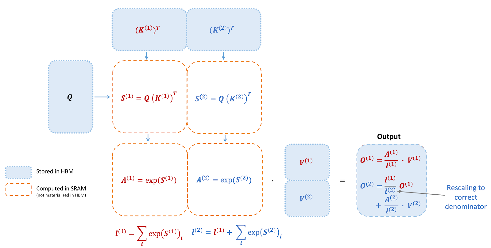
In theory, Attention is All You Need. In practice, however, we also need optimized attention implementations like FlashAttention.
Although these fused attention implementations have substantially improved performance and enabled long contexts, this efficiency has come with a loss of flexibility. You can no longer try out a new attention variant by writing a few PyTorch operators – you often need to write a new custom kernel! This operates as a sort of “software lottery” for ML researchers – if your attention variant doesn’t fit into one of the existing optimized kernels, you’re doomed to slow runtime and CUDA OOMs.
For some examples of attention variants, we have Causal, Relative Positional Embeddings, Alibi, Sliding Window Attention, PrefixLM, Document Masking/Sample Packing/Jagged Tensors, Tanh Soft-Capping, PagedAttention, etc. Even worse, folks often want combinations of these! Sliding Window Attention + Document Masking + Causal + Context Parallelism? Or what about PagedAttention + Sliding Window + Tanh Soft-Capping?
The left picture below represents the state of the world today – some combinations of masking + biases + setting have existing kernels implemented. But the various options lead to an exponential number of settings, and so overall we end up with fairly spotty support. Even worse, new attention variants researchers come up with will have zero support.
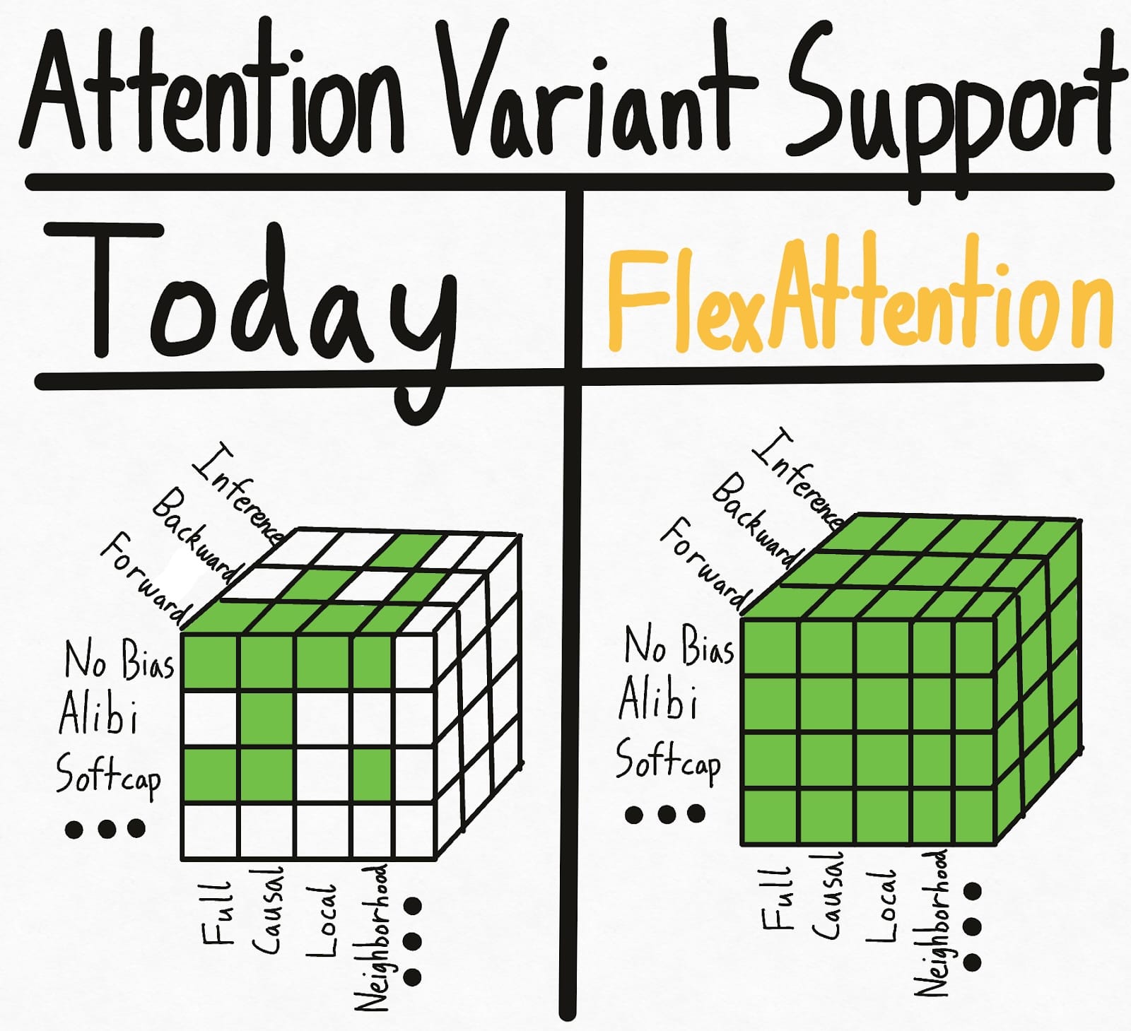
To solve this hypercube problem once and for all, we introduce FlexAttention, a new PyTorch API.
- We provide a flexible API that allows implementing many attention variants (including all the ones mentioned in the blog post so far) in a few lines of idiomatic PyTorch code.
- We lower this into a fused FlashAttention kernel through
torch.compile, generating a FlashAttention kernel that doesn’t materialize any extra memory and has performance competitive with handwritten ones.
- We also automatically generate the backwards pass, leveraging PyTorch’s autograd machinery.
- Finally, we can also take advantage of sparsity in the attention mask, resulting in significant improvements over standard attention implementations.
With FlexAttention, we hope that trying new attention variants will only be limited by your imagination.
You can find many FlexAttention examples at the Attention Gym: https://github.com/pytorch-labs/attention-gym. If you have any cool applications, feel free to submit an example!
PS: We also find this API very exciting since it leverages a lot of existing PyTorch infra in a fun way – more on that in the end.
FlexAttention
Here is the classic attention equation:
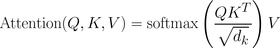
In code form:
Q, K, V: Tensor[batch_size, num_heads, sequence_length, head_dim]
score: Tensor[batch_size, num_heads, sequence_length, sequence_length] = (Q @ K) / sqrt(head_dim)
probabilities = softmax(score, dim=-1)
output: Tensor[batch_size, num_heads, sequence_length, head_dim] = probabilities @ V
FlexAttention allows for an user-defined function score_mod:
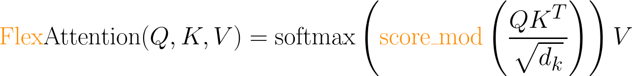
In code form:
Q, K, V: Tensor[batch_size, num_heads, sequence_length, head_dim]
score: Tensor[batch_size, num_heads, sequence_length, sequence_length] = (Q @ K) / sqrt(head_dim)
modified_scores: Tensor[batch_size, num_heads, sequence_length, sequence_length] = score_mod(score)
probabilities = softmax(modified_scores, dim=-1)
output: Tensor[batch_size, num_heads, sequence_length, head_dim] = probabilities @ V
This function allows you to modify the attention scores prior to softmax. Surprisingly, this ends up being sufficient for the vast majority of attention variants (examples below)!
Concretely, the expected signature for score_mod is somewhat unique.
def score_mod(score: f32[], b: i32[], h: i32[], q_idx: i32[], kv_idx: i32[])
    return score # noop - standard attention
In other words, score is a scalar pytorch tensor that represents the dot product of a query token and a key token. The rest of the arguments tell you which dot product you’re currently computing – b (current element in batch), h (current head), q_idx (position in query), kv_idx (position in key/value tensors).
To apply this function, we could implement it as
for b in range(batch_size):
    for h in range(num_heads):
        for q_idx in range(sequence_length):
            for kv_idx in range(sequence_length):
                modified_scores[b, h, q_idx, kv_idx] = score_mod(scores[b, h, q_idx, kv_idx], b, h, q_idx, kv_idx)
Of course, this is not how FlexAttention is implemented under the hood. Leveraging torch.compile, we automatically lower your function into a single fused FlexAttention kernel – guaranteed or your money back!
This API ends up being surprisingly expressive. Let’s look at some examples.
Score Mod Examples
Full Attention
Let’s first do “full attention”, or standard bidirectional attention. In this case, score_mod is a no-op – it takes as input the scores and then returns them as is..
def noop(score, b, h, q_idx, kv_idx):
    return score
And to use it end to end (including both forwards and backwards):
from torch.nn.attention.flex_attention import flex_attention

flex_attention(query, key, value, score_mod=noop).sum().backward()
Relative Position Encodings
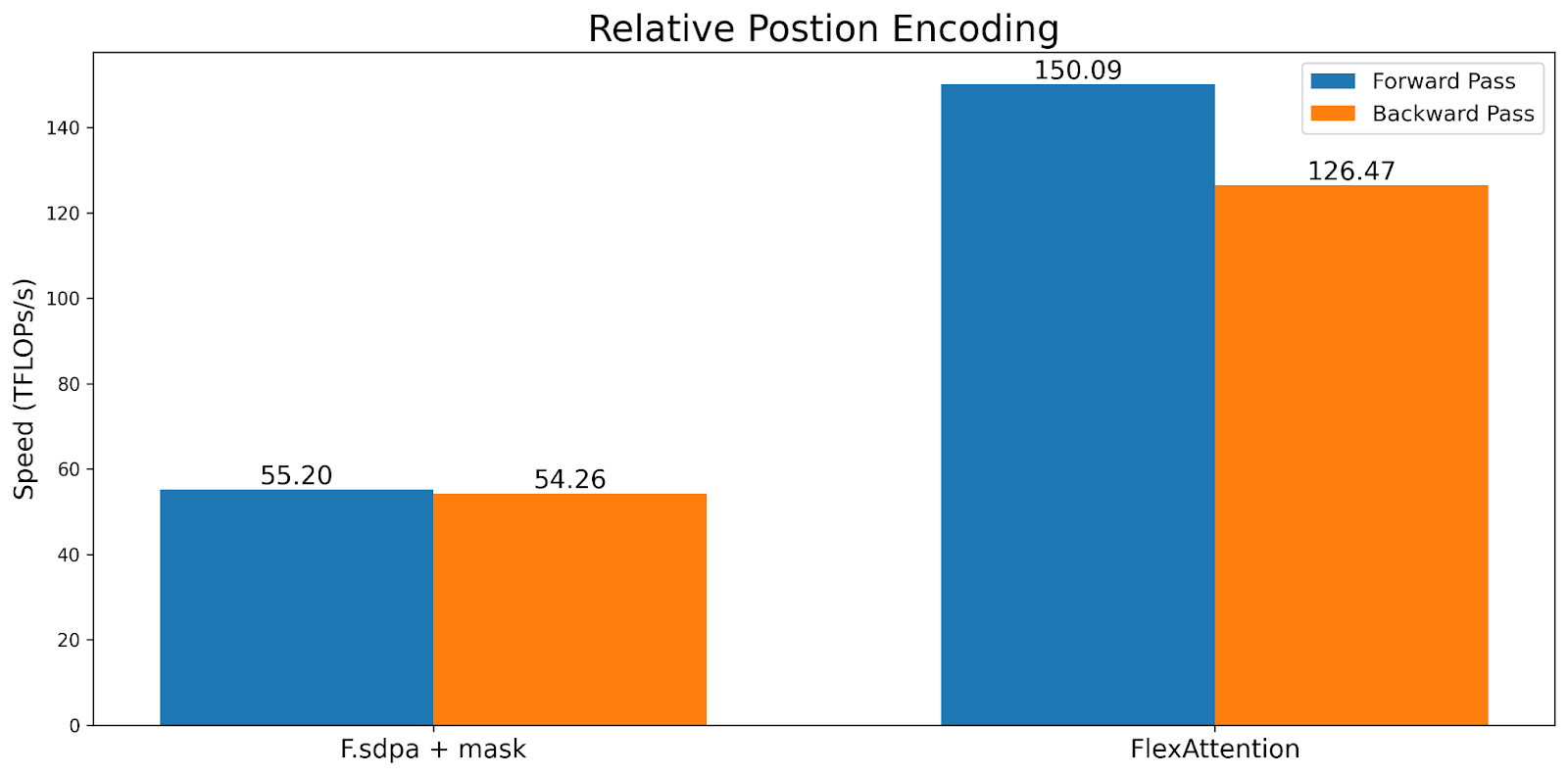
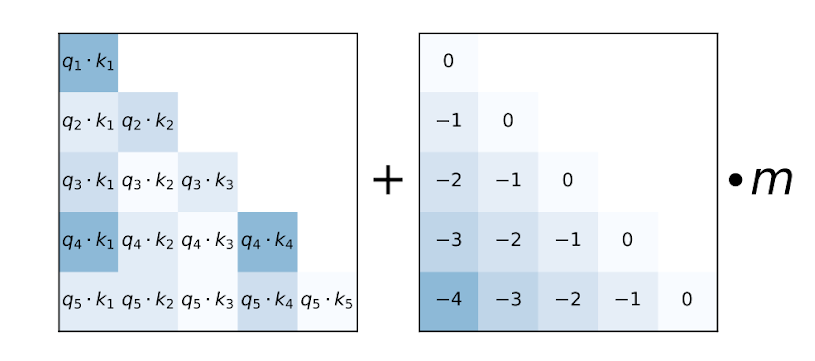
One common attention variant is the “relative position encoding”. Instead of encoding the absolute distance in the queries and keys, relative position encoding adjusts scores based on the “distance” between the queries and keys.
def relative_positional(score, b, h, q_idx, kv_idx):
    return score + (q_idx - kv_idx)
Note that unlike typical implementations, this does not need to materialize a SxS tensor. Instead, FlexAttention computes the bias values “on the fly” within the kernel, leading to significant memory and performance improvements.
ALiBi Bias
Source: Train Short, Test Long: Attention with Linear Biases Enables Input Length Extrapolation
ALiBi was introduced in Train Short, Test Long: Attention with Linear Biases Enables Input Length Extrapolation, and claims to have beneficial properties for length extrapolation at inference. Notably, MosaicML has pointed to “lack of kernel support” as the main reason why they eventually switched from ALiBi to rotary embeddings.
Alibi is similar to relative positional encodings with one exception – it has a per-head factor that is typically precomputed.
alibi_bias = generate_alibi_bias() # [num_heads]

def alibi(score, b, h, q_idx, kv_idx):
    bias = alibi_bias[h] * (q_idx - kv_idx)
    return score + bias
This demonstrates one interesting piece of flexibility torch.compile provides – we can load from alibi_bias even though it wasn’t explicitly passed in as an input! The generated Triton kernel will calculate the correct loads from the alibi_bias tensor and fuse it. Note that you could regenerate alibi_bias and we still wouldn’t need to recompile.
Soft-capping
Soft-capping is a technique used in Gemma2 and Grok-1 that prevents logits from growing excessively large. In FlexAttention, it looks like:
softcap = 20
def soft_cap(score, b, h, q_idx, kv_idx):
    score = score / softcap
    score = torch.tanh(score)
    score = score * softcap
    return score
Note that we also automatically generate the backwards pass from the forwards pass here. Also, although this implementation is semantically correct, we likely want to use a tanh approximation in this case for performance reasons. See attention-gym for more details.
Causal Mask
Although bidirectional attention is the simplest, the original Attention is All You Need paper and the vast majority of LLMs use attention in a decoder-only setting where each token can only attend to the tokens prior to it. Folks often think of this as a lower-triangular mask, but with the score_mod API it can be expressed as:
def causal_mask(score, b, h, q_idx, kv_idx):
    return torch.where(q_idx >= kv_idx, score, -float("inf"))
Basically, if the query token is “after” the key token, we keep the score. Otherwise, we mask it out by setting it to -inf, thus ensuring it won’t participate in the softmax calculation.
However, masking is special compared to other modifications – if something is masked out, we can completely skip its computation! In this case, a causal mask has about 50% sparsity, so not taking advantage of the sparsity would result in a 2x slowdown. Although this score_mod is sufficient to implement causal masking correctly, getting the performance benefits of sparsity requires another concept – mask_mod.
Mask Mods
To take advantage of sparsity from masking, we need to do some more work. Specifically, by passing a mask_mod to create_block_mask, we can create a BlockMask. FlexAttention can then use BlockMask to take advantage of the sparsity!
The signature of mask_mod is very similar to score_mod – just without the score. In particular
# returns True if this position should participate in the computation
mask_mod(b, h, q_idx, kv_idx) => bool
Note that score_mod is strictly more expressive than mask_mod. However, for masking, it’s recommended to use mask_mod and create_block_mask, as it’s more performant. See the FAQ on why score_mod and mask_mod are separate.
Now, let’s take a look at how we might implement causal mask with mask_mod.
Causal Mask
from torch.nn.attention.flex_attention import create_block_mask

def causal(b, h, q_idx, kv_idx):
    return q_idx >= kv_idx

# Because the sparsity pattern is independent of batch and heads, we'll set them to None (which broadcasts them)
block_mask = create_block_mask(causal, B=None, H=None, Q_LEN=1024, KV_LEN=1024)
# In this case, we don't need a score_mod, so we won't pass any in.
# However, score_mod can still be combined with block_mask if you need the additional flexibility.
flex_attention(query, key, value, block_mask=block_mask)
Note that create_block_mask is a relatively expensive operation! Although FlexAttention will not need to recompile when it changes, if you aren’t careful about caching it, it can lead to significant slowdowns (check out the FAQ for suggestions on best practices).
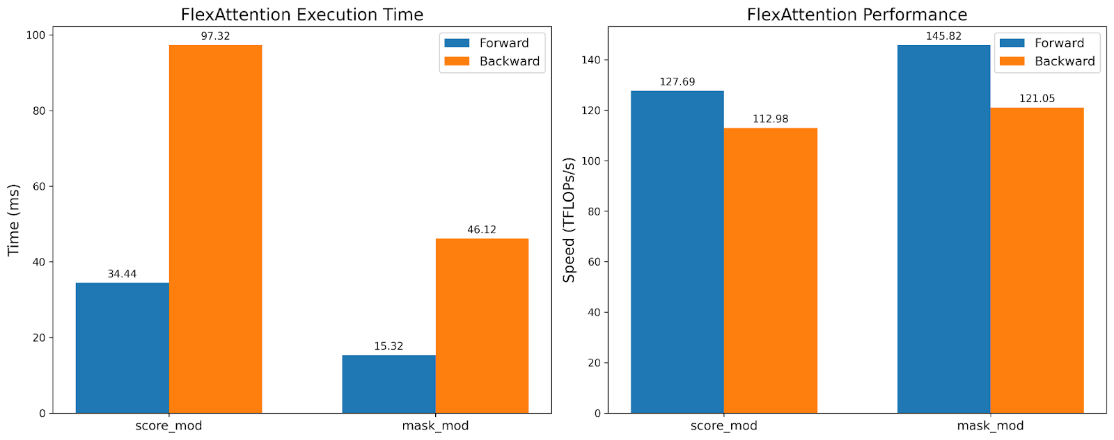
While the TFlops are roughly the same, the execution time is 2x faster for the mask_mod version! This demonstrates that we can leverage the sparsity that BlockMask provides us without losing hardware efficiency.
Sliding Window + Causal
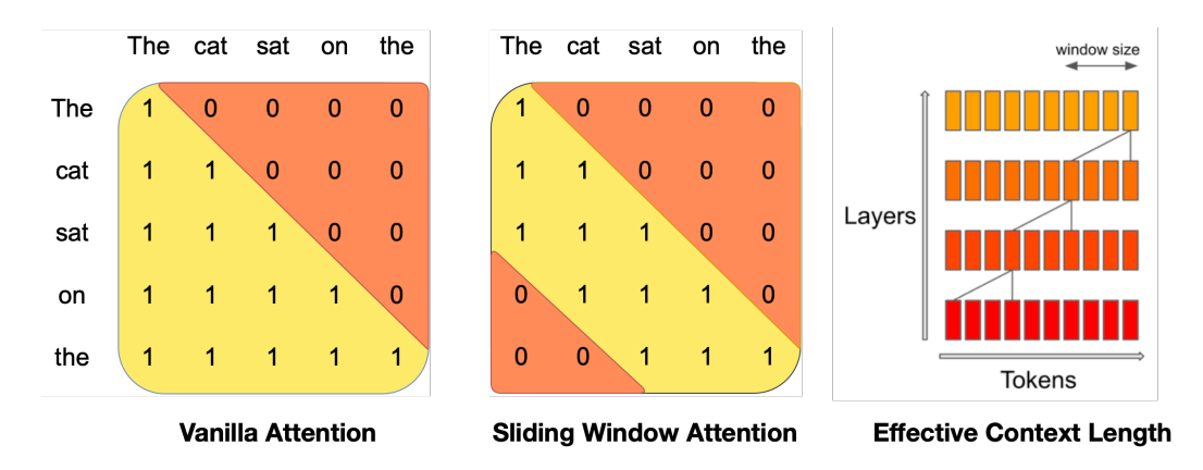
Source: Mistral 7B
Popularized by Mistral, sliding window attention (also known as local attention) takes advantage of the intuition that the most recent tokens are the most useful. In particular, it allows the query token to only attend to, say, the 1024 most recent tokens. This is often used together with causal attention.
SLIDING_WINDOW = 1024

def sliding_window_causal(b, h, q_idx, kv_idx):
    causal_mask = q_idx >= kv_idx
    window_mask = q_idx - kv_idx <= SLIDING_WINDOW
    return causal_mask & window_mask

# If you want to be cute...
from torch.nn.attention import or_masks

def sliding_window(b, h, q_idx, kv_idx)
    return q_idx - kv_idx <= SLIDING_WINDOW

sliding_window_causal = or_masks(causal_mask, sliding_window)
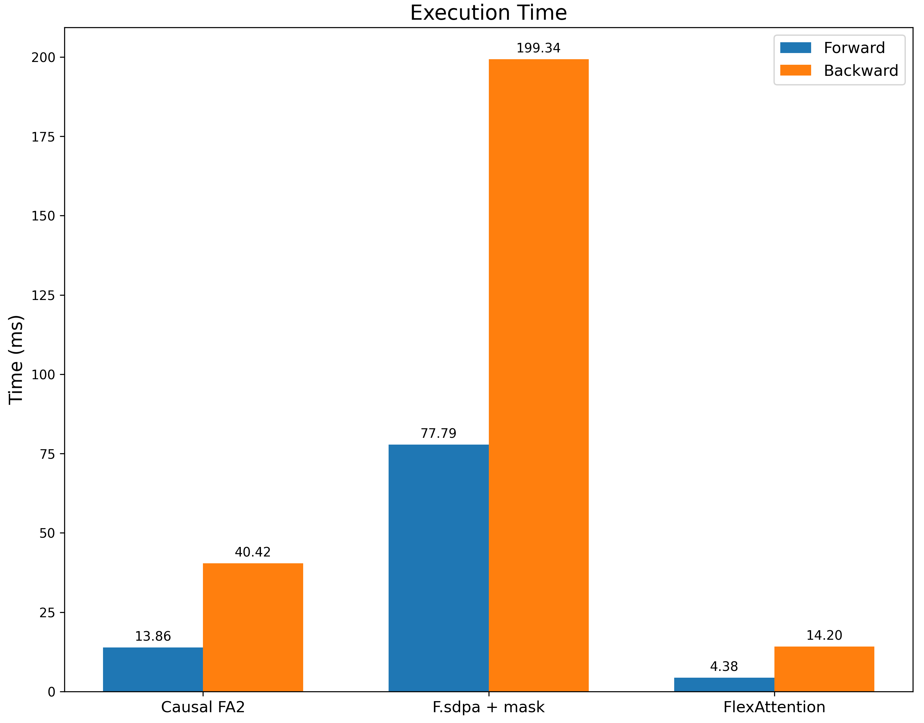
We benchmark it against F.scaled_dot_product_attention with a sliding window mask as well as FA2 with a causal mask (as a reference point for performance). Not only are we significantly faster than F.scaled_dot_product_attention, we’re also significantly faster than FA2 with a causal mask as this mask has significantly more sparsity.
PrefixLM
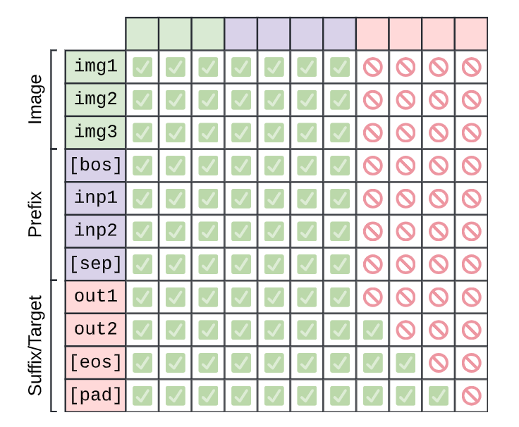
Source: PaliGemma: A versatile 3B VLM for transfer
The T5 architecture, proposed in Exploring the Limits of Transfer Learning with a Unified Text-to-Text Transformer, describes an attention variant that performs full bidirectional attention on a “prefix”, and causal attention on the rest. We again compose two mask functions to accomplish this, one for causal masking and one that is based off of the prefix length.
prefix_length: [B]
def prefix_mask(b, h, q_idx, kv_idx):
    return kv_idx <= prefix_length[b]

prefix_lm_causal = or_masks(prefix_mask, causal_mask)
# In this case, our mask is different per sequence so we set B equal to our batch size
block_mask = create_block_mask(prefix_lm_causal, B=B, H=None, S, S)
Just like with score_mod, mask_mod allows us to refer to additional tensors that aren’t explicitly an input to the function! However, with prefixLM, the sparsity pattern changes per input. This means that for each new input batch, we’ll need to recompute the BlockMask. One common pattern is to call create_block_mask at the beginning of your model and reuse that block_mask for all attention calls in your model. See Recomputing Block Masks vs. Recompilation.
However, in exchange for that, we’re not only able to have an efficient attention kernel for prefixLM, we’re also able to take advantage of however much sparsity exists in the input! FlexAttention will dynamically adjust its performance based off of the BlockMask data, without needing to recompile the kernel.
Document Masking/Jagged Sequences
Another common attention variant is document masking/jagged sequences. Imagine that you have a number of sequences of varying length. You want to train on all of them together, but unfortunately, most operators only accept rectangular tensors.
Through BlockMask, we can support this efficiently in FlexAttention as well!
- First, we flatten all sequences into a single sequence with sum(sequence lengths) tokens.
- Then, we compute the document_id that each token belongs to.
- Finally, in our
mask_mod, we simply whether the query and kv token belong to the same document!
# The document that each token belongs to.
# e.g. [0, 0, 0, 1, 1, 2, 2, 2, 2, 2, 2] corresponds to sequence lengths 3, 2, and 6.
document_id: [SEQ_LEN]
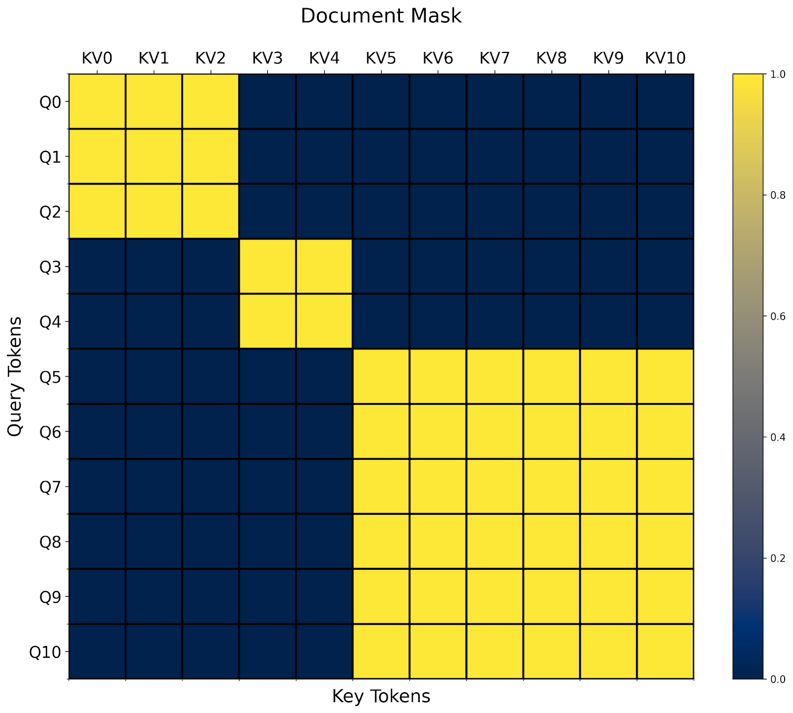
def document_masking(b, h, q_idx, kv_idx):
return document_id[q_idx] == document_id[kv_idx]
And that’s it! In this case, we see that we end up with a blockdiagonal mask.
One interesting aspect about document masking is that it’s easy to see how it might combine with an arbitrary combination of other masks . For example, we already defined prefixlm_mask in the previous section. Do we now need to define a prefixlm_document_mask function as well?
In these cases, one pattern we’ve found quite useful is what we call a “higher level modification”. In this case, we can take an existing mask_mod and automatically transform it into one that works with jagged sequences!
def generate_doc_mask_mod(mask_mod, document_id):
    # Get unique document IDs and their counts
    _, counts = torch.unique_consecutive(document_id, return_counts=True)
    # Create cumulative counts (offsets)
    offsets = torch.cat([torch.tensor([0], device=document_id.device), counts.cumsum(0)[:-1]])
    def doc_mask_wrapper(b, h, q_idx, kv_idx):
        same_doc = document_id[q_idx] == document_id[kv_idx]
        q_logical = q_idx - offsets[document_id[q_idx]]
        kv_logical = kv_idx - offsets[document_id[kv_idx]]
        inner_mask = mask_mod(b, h, q_logical, kv_logical)
        return same_doc & inner_mask
    return doc_mask_wrapper
For example, given the prefix_lm_causal mask from above, we can transform it into one that works on on packed documents like so:
prefix_length = torch.tensor(2, dtype=torch.int32, device="cuda")
def prefix_mask(b, h, q_idx, kv_idx):
    return kv_idx < prefix_length
prefix_lm_causal = or_masks(prefix_mask, causal_mask)
doc_prefix_lm_causal_mask = generate_doc_mask_mod(prefix_lm_causal, document_id)
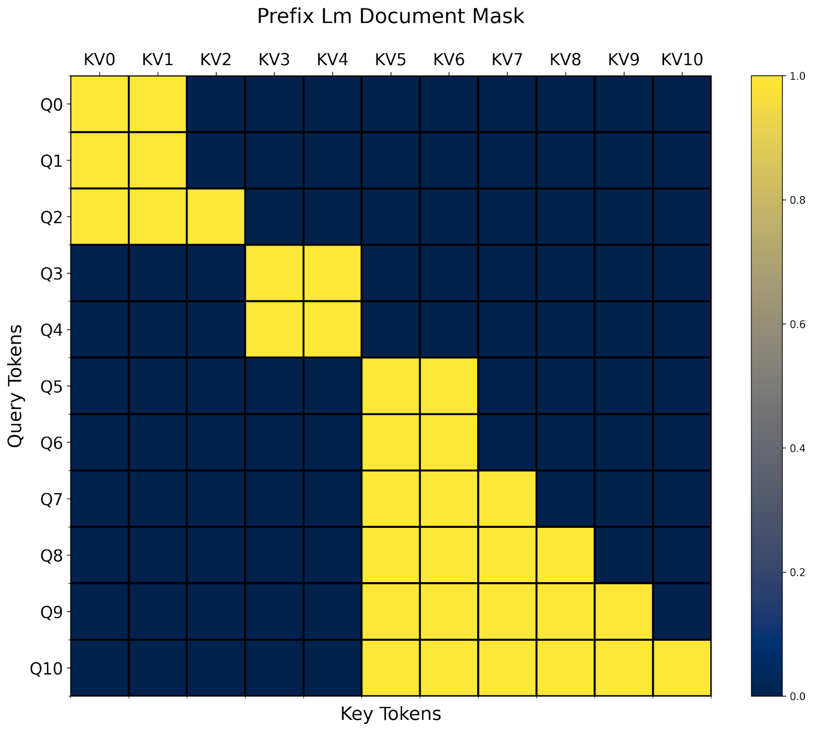
Now, this mask is “block-prefixLM-diagonal” shaped. 🙂
That’s all of our examples! There are far more attention variants than we have space to list, so check out Attention Gym for more examples. We hope that the community will contribute some of their favorite applications of FlexAttention as well.
FAQ
Q: When does FlexAttention need to recompile?
As FlexAttention leverages torch.compile for graph capture, it can actually avoid recompilation in a broad spectrum of cases. Notably, it does not need to recompile even if captured tensors change values!
flex_attention = torch.compile(flex_attention)
def create_bias_mod(bias)
    def bias_mod(score, b, h, q_idx, kv_idx):
        return score + bias
    return bias_mod
bias_mod1 = create_bias_mod(torch.tensor(0))
flex_attention(..., score_mod=bias_mod1) # Compiles the kernel here

bias_mod2 = create_bias_mod(torch.tensor(2))
flex_attention(..., score_mod=bias_mod2) # Doesn't need to recompile!
Even changing the block-sparsity doesn’t require a recompile. However, if the block-sparsity changes, we do need to recompute the BlockMask.
Q: When should we recompute the BlockMask?
We need to recompute the BlockMask whenever the block-sparsity changes. Although computing the BlockMask is much cheaper than recompilation (on the order of hundreds of microseconds as opposed to seconds), you should still take care to not excessively recompute the BlockMask.
Here are some common patterns and some recommendations on how you might approach them.
Mask never changes (e.g. causal mask)
In this case, you can simply precompute the block mask and cache it globally, reusing it for all attention calls.
block_mask = create_block_mask(causal_mask, 1, 1, S,S)
causal_attention = functools.partial(flex_attention, block_mask=block_mask)
Mask changes every batch (e.g. document masking)
In this case, we would suggest computing the BlockMask at the beginning of the model and threading it through the model – reusing the BlockMask for all layers.
def forward(self, x, doc_mask):
    # Compute block mask at beginning of forwards
    block_mask = create_block_mask(doc_mask, None, None, S, S)
    x = self.layer1(x, block_mask)
    x = self.layer2(x, block_mask)
    ...
    # amortize block mask construction cost across all layers
    x = self.layer3(x, block_mask)
    return x
Mask changes every layer (e.g. data-dependent sparsity)
This is the hardest setting, since we’re unable to amortize the block mask computation across multiple FlexAttention invocations. Although FlexAttention can certainly still benefit this case, the actual benefits from BlockMask depend on how sparse your attention mask is and how fast we can construct the BlockMask. That leads us to…
Q: How can we compute BlockMask quicker?
create_block_mask is unfortunately fairly expensive, both from a memory and compute perspective, as determining whether a block is completely sparse requires evaluating mask_mod at every single point in the block. There are a couple ways to address this:
- If your mask is the same across batch size or heads, make sure that you’re broadcasting over those (i.e. set them to
None in create_block_mask).
- Compile
create_block_mask. Unfortunately, today, torch.compile does not work directly on create_block_mask due to some unfortunate limitations. However, you can set _compile=True, which will significantly reduce the peak memory and runtime (often an order of magnitude in our testing).
-
Write a custom constructor for BlockMask. The metadata for BlockMask is quite simple (see the documentation). It’s essentially two tensors.
a. num_blocks: The number of KV blocks computed for each query block.
b. indices: The positions of the KV blocks computed for each query block.
For example, here’s a custom BlockMask constructor for causal_mask.
def create_causal_mask(S):
    BLOCK_SIZE = 128
    # The first query block computes one block, the second query block computes 2 blocks, etc.
    num_blocks = torch.arange(S // BLOCK_SIZE, device="cuda") + 1
    # Since we're always computing from the left to the right,
    # we can use the indices [0, 1, 2, ...] for every query block.
    indices = torch.arange(S // BLOCK_SIZE, device="cuda").expand(
        S // BLOCK_SIZE, S // BLOCK_SIZE
    )
    num_blocks = num_blocks[None, None, :]
    indices = indices[None, None, :]
    return BlockMask(num_blocks, indices, BLOCK_SIZE=BLOCK_SIZE, mask_mod=causal_mask)
Q: Why are score_mod and mask_mod different? Isn’t mask_mod just a special case of score_mod?
Very astute question, hypothetical audience member! In fact, any mask_mod can be easily converted to a score_mod (we do not recommend using this function in practice!)
def mask_mod_as_score_mod(b, h, q_idx, kv_idx):
    return torch.where(mask_mod(b, h, q_idx, kv_idx), score, -float("inf"))
So, if score_mod can implement everything mask_mod can, what’s the point of having mask_mod?
One immediate challenge: a score_mod requires the actual score value as an input, but when we’re precomputing the BlockMask, we don’t have the actual score value. We can perhaps fake the values by passing in all zeros, and if the score_mod returns -inf, then we consider it to be masked (in fact, we originally did this!).
However, there are two issues. The first is that this is hacky – what if the user’s score_mod returned -inf when the input is 0? Or what if the user’s score_mod masked out with a large negative value instead of -inf? It seems we’re trying to cram a round peg into a square hole. However, there’s a more important reason to separate out mask_mod from score_mod – it’s fundamentally more efficient!.
As it turns out, applying masking to every single computed element is actually quite expensive – our benchmarks see about a 15-20% degradation in performance! So, although we can get significant speedups by skipping half the computation, we lose a meaningful part of that speedup from needing to mask out every element!
Luckily, if we visualize the causal mask, we notice that the vast majority of blocks do not require a “causal mask” at all – they’re fully computed! It is only the blocks on the diagonal, partially computed and partially masked, that require masking to be applied.
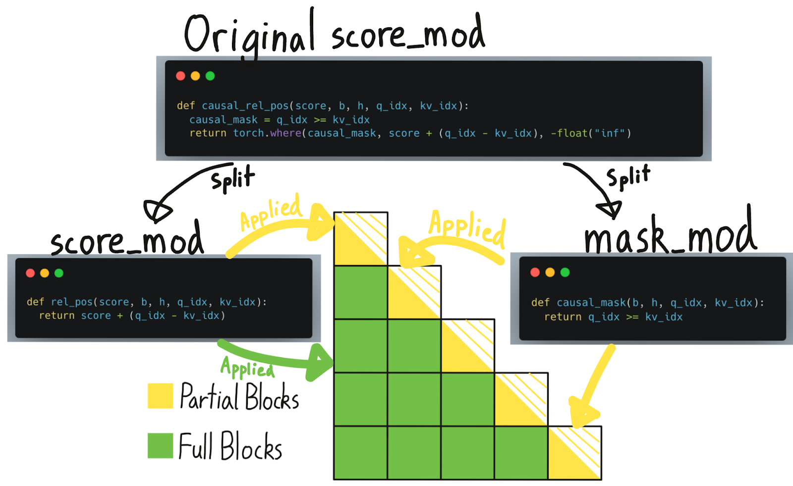
The BlockMask previously told us which blocks we need to compute and which blocks we can skip. Now, we further augment this data structure to also tell us which blocks are “fully computed” (i.e. masking can be skipped) vs. “partially computed” (i.e. a mask needs to be applied). Note, however, that although masks can be skipped on “fully computed” blocks, other score_mods like relative positional embeddings still need to be applied.
Given just a score_mod, there’s no sound way for us to tell which parts of it are “masking”. Hence, the user must separate these out themselves into mask_mod.
Q: How much additional memory does the BlockMask need?
The BlockMask metadata is of size [BATCH_SIZE, NUM_HEADS, QUERY_LEN//BLOCK_SIZE, KV_LEN//BLOCK_SIZE]. If the mask is the same across the batch or heads dimension it can be broadcasted over that dimension to save memory.
At the default BLOCK_SIZE of 128, we expect that the memory usage will be fairly negligible for most use cases. For example, for a sequence length of 1 million, the BlockMask would only use 60MB of additional memory. If this is a problem, you can increase the block size: create_block_mask(..., BLOCK_SIZE=1024). For example, increasing BLOCK_SIZE to 1024 would result in this metadata dropping to under a megabyte.
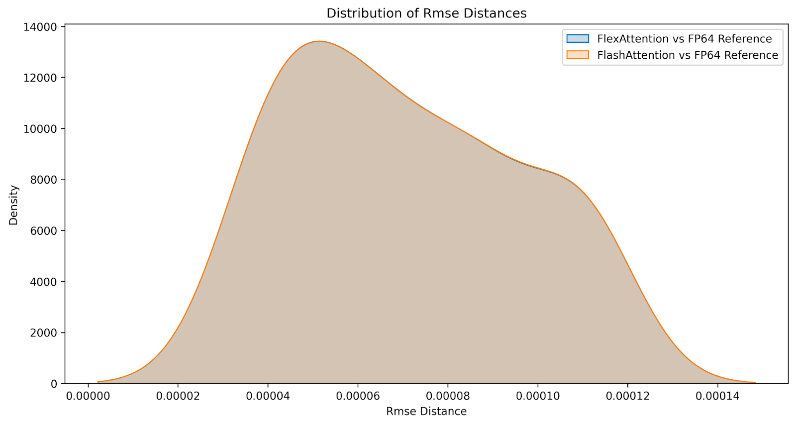
Q: How do the numerics compare?
Although the results are not bitwise identical, we are confident that FlexAttention is as numerically accurate as FlashAttention. We generate the following distribution of differences comparing FlashAttention versus FlexAttention over a large range of inputs on both causal and non causal attention variants. The errors are nearly identical.
Performance
Generally speaking, FlexAttention is nearly as performant as a handwritten Triton kernel, which is unsurprising, as we heavily leverage a handwritten Triton kernel. However, due to its generality, we do incur a small performance penalty. For example, we must incur some additional latency to determine which block to compute next. In some cases, we provide some kernel options that can affect the performance of the kernel while changing its behavior. They can be found here: performance knobs
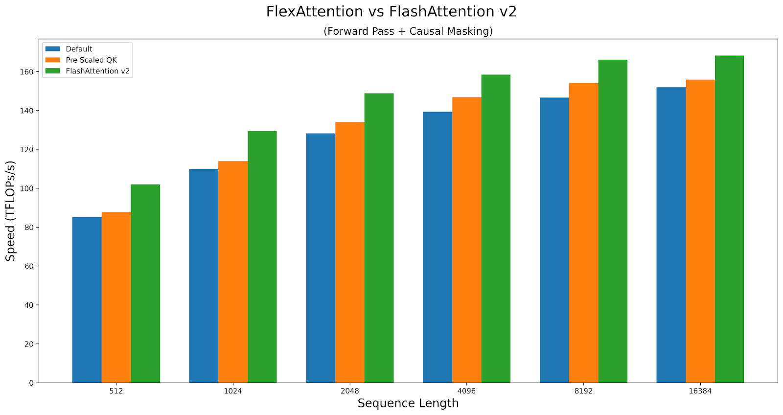
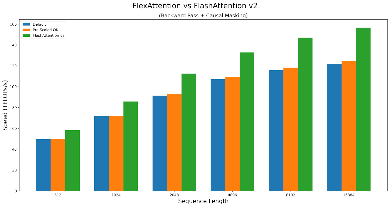
As a case study, let’s explore how the knobs affect the performance of causal attention. We will compare performance of the triton kernel versus FlashAttentionv2 on A100. The script can be found here.
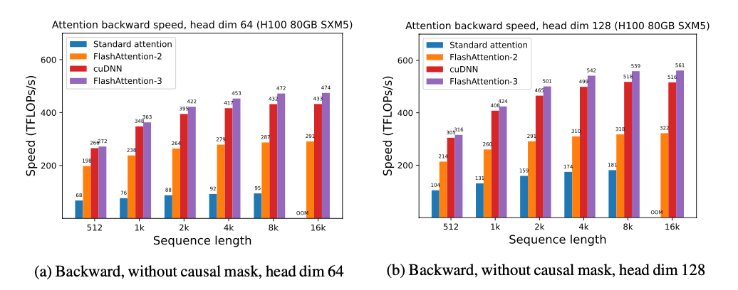
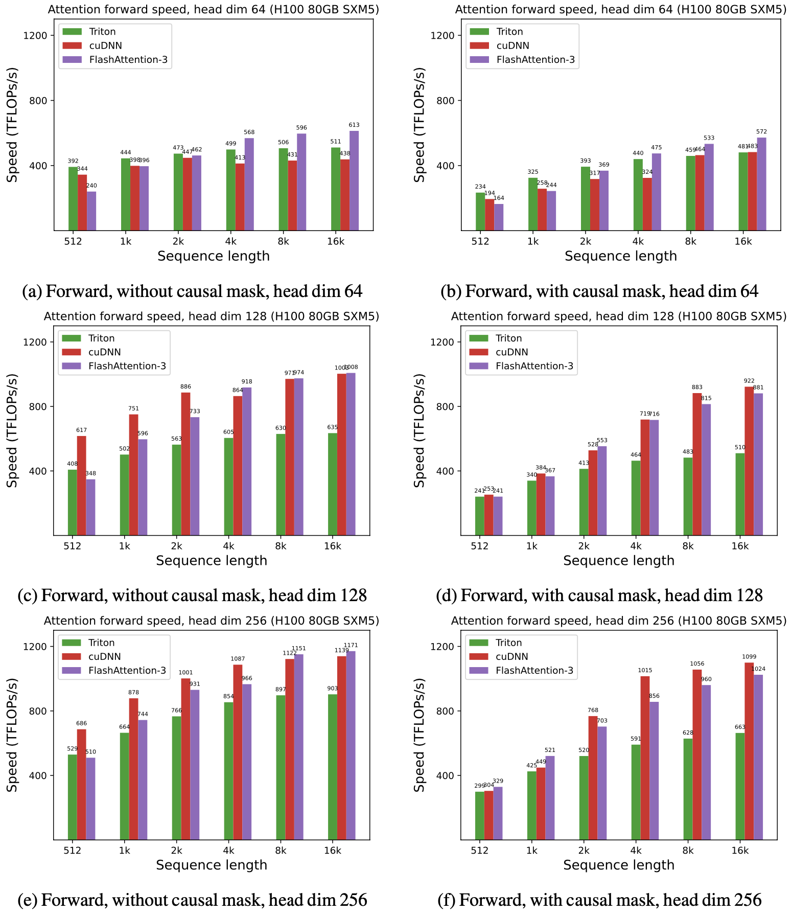
FlexAttention achieves 90% of FlashAttention2’s performance in the forward pass and 85% in the backward pass. FlexAttention is currently utilizing a deterministic algorithm that recomputes more intermediates than FAv2, but we have plans to improve FlexAttention’s backward algorithm and hope to close this gap!
Conclusion
We hope you have as much fun using FlexAttention as we did developing it! While working on this, we ended up finding way more applications of this API than we could have expected. We’ve already seen it accelerate torchtune’s sample packing throughput by 71%, replace the need for a researcher to spend over a week writing their own custom Triton kernel, and deliver competitive performance with custom handwritten attention variants.
One final thing that made implementing FlexAttention quite fun is that we were able to leverage a lot of existing PyTorch infra in an interesting way. For example, one of the unique aspects about TorchDynamo (torch.compile’s frontend) is that it does not require tensors used in the compiled function to be explicitly passed in as inputs. This allows us to compile mods like document masking, which require accessing global variables where the global variables need to change!
bias = torch.randn(1024, 1024)
def score_mod(score, b, h, q_idx, kv_idx):
    return score + bias[q_idx][kv_idx] # The bias tensor can change!
Furthermore, the fact that torch.compile is a generic graph-capture mechanism also allows it to support more “advanced” transformations, such as the higher order transform that transforms any mask_mod into one that works with jagged tensors.
We also leverage TorchInductor (torch.compile’s backend) infrastructure for Triton templates. Not only did this make it easy to support codegening FlexAttention – it also automatically gave us support for dynamic shapes as well as epilogue fusion (i.e. fusing an operator onto the end of attention)! In the future, we plan on extending this support to allow for quantized versions of attention or things like RadixAttention as well.
In addition, we also leveraged higher order ops, PyTorch’s autograd to automatically generate the backwards pass, as well as vmap to automatically apply score_mod for creating the BlockMask.
And, of course, this project wouldn’t have been possible without Triton and TorchInductor’s ability to generate Triton code.
We look forward to leveraging the approach we used here to more applications in the future!
Limitations and Future Work
- FlexAttention is currently available in PyTorch nightly releases, we plan to release it as a prototype feature in 2.5.0
- We did not cover how to use FlexAttention for inference here (or how to implement PagedAttention) – we will cover those in a later post.
- We are working to improve the performance of FlexAttention to match FlashAttention3 on H100 GPUs.
- FlexAttention requires that all sequence lengths be a multiple of 128 – this will be addressed soon.
- We plan on adding GQA support soon – for now, you can just replicate the kv heads.
Acknowledgements
We want to highlight some prior work (and people) that have inspired FlexAttention.
- Tri Dao’s work on FlashAttention
- Francisco Massa and the Xformers team for BlockSparseAttention in Triton
- The Jax team’s work on SplashAttention
- Philippe Tillet and Keren Zhou for helping us with Triton
- Ali Hassani for discussions on neighborhood attention
- Everybody who’s complained about attention kernels not supporting their favorite attention variant 🙂
Read More