TLDR
- ExecuTorch has achieved Beta status with the release of v0.4, providing stable APIs and runtime, as well as extensive kernel coverage.
- ExecuTorch is the recommended on-device inference engine for Llama 3.2 1B/3B models, offering enhanced performance and memory efficiency for both original and quantized models.
- There has been a significant increase in adoption and ecosystem growth for ExecuTorch, and the focus is now on improving reliability, performance, and coverage for non-CPU backends as the next steps.
Current On-Device AI Market
The on-device AI market has been rapidly expanding, and is revolutionizing the way we interact with technology. It is unlocking new experiences, enabling personalization, and reducing latency. Traditionally, computer vision and speech recognition have been the primary use-cases for on-device AI, particularly in IoT, industrial applications, and mobile devices. However, the emergence of Large Language Models (LLMs) has made Generative AI the fastest growing sector in AI, subsequently highlighting the importance of on-device Generative AI. IDC forecasts by 2028, close to 1 billion GenAI capable smartphones being shipped worldwide.
LLMs are not only getting smaller but more powerful. This has led to the creation of a new class of applications that leverage multiple models for intelligent agents and streamlined workflows. The community is rapidly adopting and contributing to these new models, with quantized versions being created within hours of model release. Several leading technology companies are investing heavily in small LLMs, even deploying Low-Rank Adaptation (LoRA) at scale on-device to transform user experiences.
However, this rapid progress comes at a cost. The fragmentation of our on-device AI landscape creates complexity and inefficiency when going from model authoring to edge deployment. This is where PyTorch’s ExecuTorch comes in – our Beta announcement marks an important milestone in addressing these challenges and empowering developers to create innovative, AI-powered applications.
What’s New Today
It’s been exactly one year since we first open sourced ExecuTorch, six months since Alpha release, and today, we’re excited to announce three main developments:
1. Beta. ExecuTorch has reached Beta status starting from v0.4! It is now widely adopted and used in production environments across Meta. Through this adoption process we’ve identified and addressed feature gaps, improved stability, and expanded kernel and accelerator coverage. These improvements make us confident to promote ExecuTorch from Alpha to Beta status, and we are happy to welcome the community to adopt it in their own production settings. Here are three concrete enhancements:
- Developers can write application code and include the latest ExecuTorch as a dependency, updating when needed with a clean API contract. This is possible due to our API stabilization efforts, as well as our explicit API lifecycle and backwards compatibility policy.
- Running ExecuTorch on CPUs reached the necessary performance, portability and coverage. In particular, we have implemented more than 85% of all core ATen operators as part of our portable CPU kernels library to ensure running a model on ExecuTorch just works in most cases and making missing ops an exception rather than the norm. Moreover, we integrated and extensively tested our XNNPACK delegate for high performance on a wide range of CPU architectures. It is used in a number of production cases today.
- In addition to the low-level ExecuTorch components for greater portability, we built extensions and higher-level abstractions to support more common use-cases such as developer tooling to support on-device debugging and profiling, and Module.h extension to simplify deployment for mobile devices.
2. On-Device Large-Language Models (LLMs). There has been a growing interest in the community to deploy Large Language Models (LLMs) on edge devices, as it offers improved privacy and offline capabilities. However, these models are quite large, pushing the limits of what is possible. Fortunately, ExecuTorch can support these models, and we’ve enhanced the overall framework with numerous optimizations.
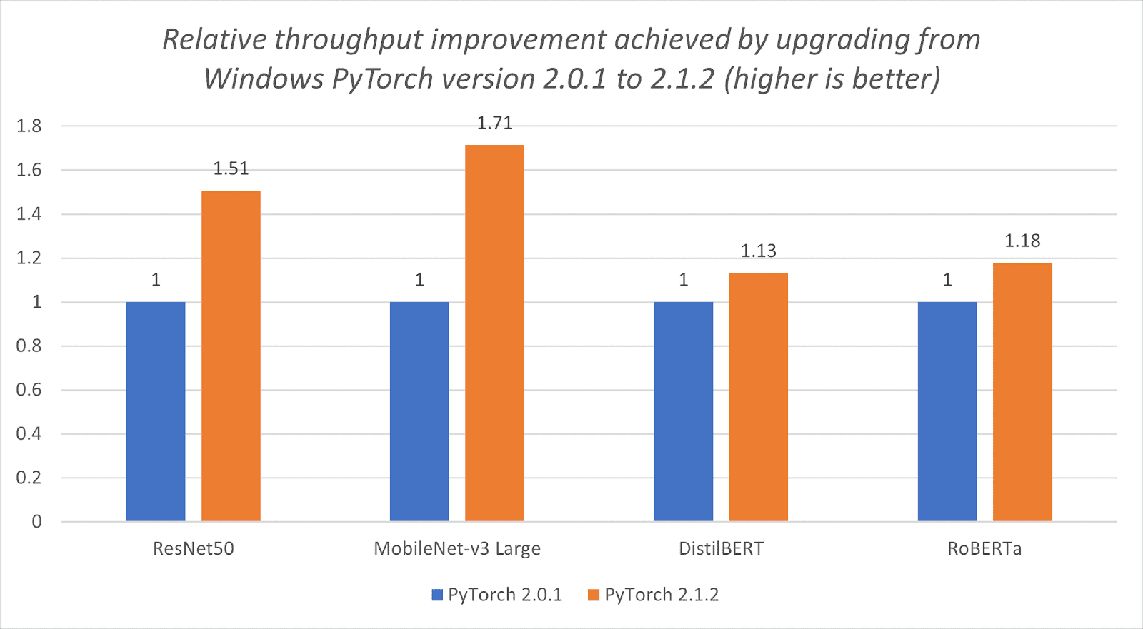
- ExecuTorch is the recommended framework to run latest Llama models on-device with excellent performance today. The Llama 3.2 1B/3B models are well-suited for mobile deployment, and it is especially true with the official quantized 1B/3B model releases from Meta, as it provides a great balance between performance, accuracy, and size. When deploying Llama 3.2 1B/3B quantized models, decode latency improved by 2.5x and prefill latency improved by 4.2x on average, while model size decreased by 56% and memory usage reduced by 41% on average when benchmarked on Android OnePlus 12 device (we’ve also verified similar relative performance on Samsung S24+ for 1B and 3B, and Samsung S22 for 1B). For Llama 3.2 1B quantized model, for example, ExecuTorch is able to achieve 50.2 tokens/s for decoding and 260 tokens/s for prefill on the OnePlus 12, using the latest CPU kernels from XNNPACK and Kleidi libraries. These quantized models allow developers to integrate LLMs into memory and power-constrained devices while still maintaining quality and safety.
- One of the value propositions of ExecuTorch is being able to use accelerators on mobile devices seamlessly. In fact, ExecuTorch also showcased accelerators to achieve even greater performance running Llama across Apple MPS backend, Qualcomm AI Accelerator, and MediaTek AI Accelerator.
- There has been growing community and industry interest in multimodal and beyond text-only LLMs, evidenced by Meta’s Llama 3.2 11B/90B vision models and open-source models like Llava. We have so far enabled Llava 1.5 7B model on phones via ExecuTorch, making many optimizations, notably reducing runtime memory from 11GB all the way down to 5GB.
3. Ecosystem and Community Adoption
Now that ExecuTorch is in Beta, it is mature enough to be used in production. It is being increasingly used at Meta across various product surfaces. For instance, ExecuTorch already powers various ML inference use cases across Meta’s Ray-Ban Meta Smart Glasses and Quest 3 VR headsets as well as Instagram and WhatsApp.
We also partnered with Hugging Face to provide native ExecuTorch support for models being exported using torch.export. This collaboration ensures exported artifacts can directly be lowered and run efficiently on various mobile and edge devices. Models like gemma-2b and phi3-mini are already supported and more foundational models support is in progress.
With stable APIs and Gen AI support, we’re excited to build and grow ExecuTorch with the community. The on-device AI community is growing rapidly and finding ways to adopt ExecuTorch across various fields. For instance, ExecuTorch is being used in a mobile app built by Digica to streamline inventory management in hospitals. As another example, Software Mansion developed an app, EraserAI, to remove unwanted objects from a photo with EfficientSAM running on-device with ExecuTorch via Core ML delegate.
Towards General Availability (GA):
Since the original release of ExecuTorch alpha, we’ve seen a growing interest within the community in using ExecuTorch in various production environments. To that end, we have made great progress towards more stabilized and matured APIs and have made a significant investment in community support, adoption and contribution to ExecuTorch. As are are getting close to GA, we are investing our efforts in the following areas:
-
Non-CPU backends: Bringing non-CPU backends to even greater robustness, coverage and performance is our next goal. From day one of our original launch, we have partnered with Apple (for Core ML and MPS), Arm (for EthosU NPU) and Qualcomm (for Hexagon NPU) on accelerator integration with ExecuTorch, and we’ve since then expanded our partnership to MediaTek (NPU) and Cadence (XTensa DSP). We’re also building Vulkan GPU integration in-house. In terms of feature coverage, we’ve successfully implemented the core functionalities with our partners, ensured seamless integration with our developer tooling, and showcased successful LLM integration with many of the accelerators. Our next big step is to thoroughly validate the performance and reliability of the system in real-world, production use-cases. This stage will help us fine-tune the experience and ensure the stability needed for smooth operations.
-
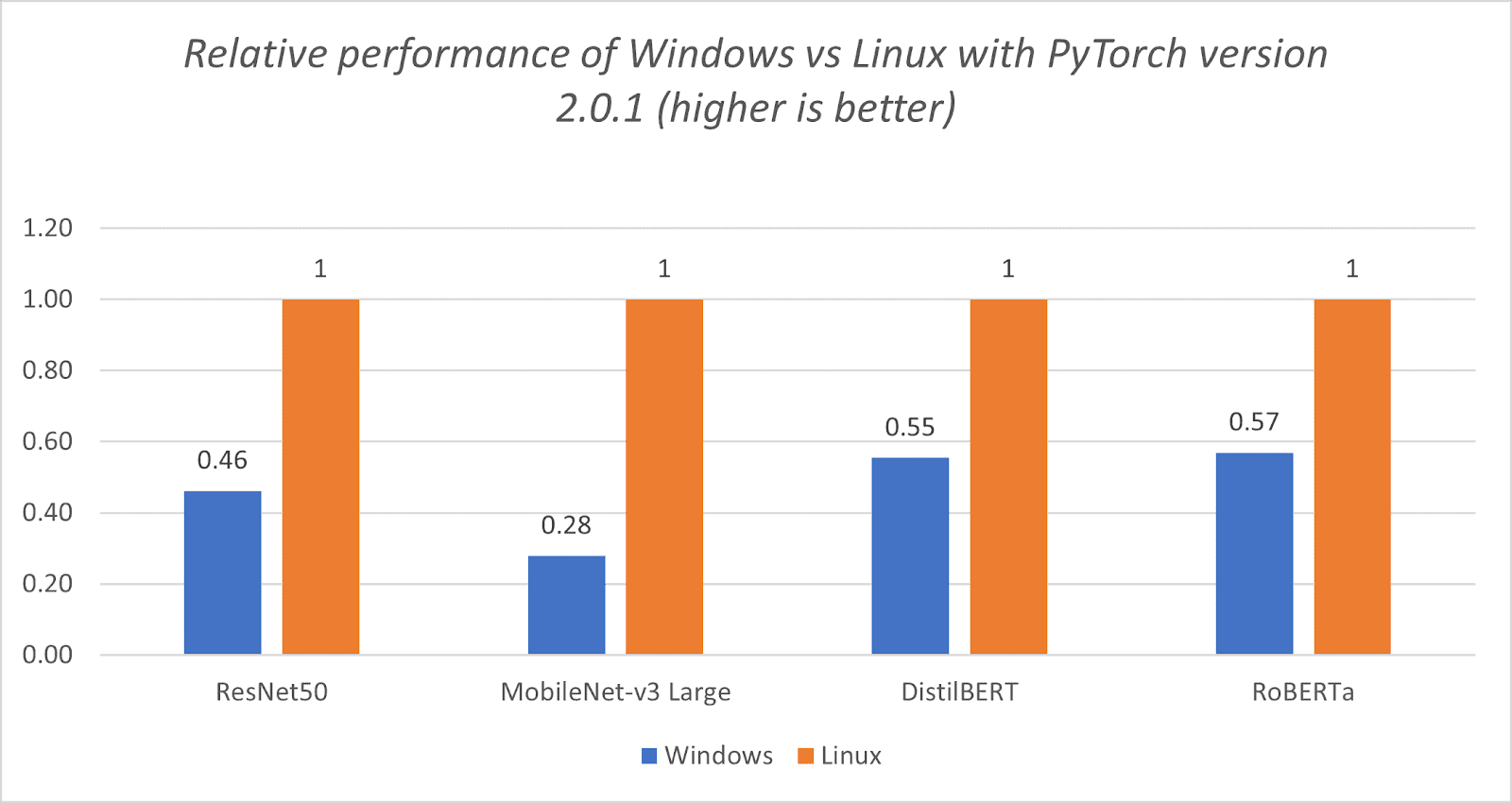
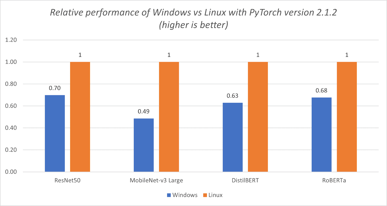
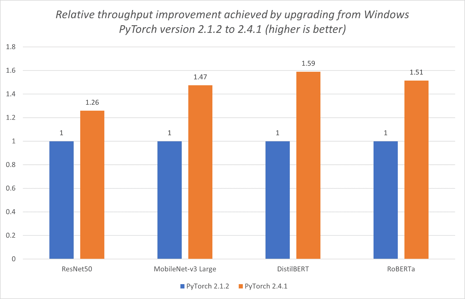
Benchmarking infra: As part of our ongoing testing efforts, we’ve developed a benchmarking infrastructure along with a public dashboard to showcase our progress toward on-device model inference benchmarking. This allows us to transparently track and display model coverage across various backends, giving our community real-time insights into how we’re advancing towards our goals.
We’re excited to share these developments with you and look forward to continued improvements in collaboration with our partners and the community! We welcome community contribution to help us make ExecuTorch the clear choice for deploying AI and LLM models on-device. We invite you to start using ExecuTorch in your on-device projects, or even better consider contributing to it. You can also report any issues on our GitHub page.