This blog is the fifth in a series focused on accelerating generative AI models with pure, native PyTorch. We demonstrate the GenAI acceleration of GPTFast, Segment Anything Fast, and Diffusion Fast on Intel® Xeon®Processors.
First, we revisit GPTFast, a remarkable work that speeds up text generation in under 1000 lines of native PyTorch code. Initially, GPTFast supported only the CUDA backend. We will show you how to run GPTFast on CPU and achieve additional performance speedup with weight-only quantization (WOQ).
In Segment Anything Fast, we have incorporated support for the CPU backend and will demonstrate performance acceleration by leveraging the increased power of CPU with BFloat16, torch.compile, and scaled_dot_product_attention (SDPA) with a block-wise attention mask. The speedup ratio against FP32 can reach 2.91x in vit_b and 3.95x in vit_h.
Finally, Diffusion Fast now supports the CPU backend and leverages the increased power of CPU with BFloat16, torch.compile, and SDPA. We also optimize the layout propagation rules for convolution, cat, and permute in Inductor CPU to improve performance. The speedup ratio against FP32 can achieve 3.91x in Stable Diffusion XL (SDXL).
Optimization strategies to boost performance on PyTorch CPU
GPTFast
Over the past year, generative AI has achieved great success across various language tasks and become increasingly popular. However, generative models face high inference costs due to the memory bandwidth bottlenecks in the auto-regressive decoding process. To address these issues, the PyTorch team published GPTFast which targets accelerating text generation with only pure, native PyTorch. This project developed an LLM from scratch almost 10x faster than the baseline in under 1000 lines of native PyTorch code. Initially, GPTFast supported only the CUDA backend and garnered approximately 5,000 stars in about four months. Inspired by Llama.cpp, the Intel team provided CPU backend support starting with the PyTorch 2.4 release, further enhancing the project’s availability in GPU-free environments. The following are optimization strategies used to boost performance on PyTorch CPU:
-
Torch.compile
torch.compile is a PyTorch function introduced since PyTorch 2.0 that aims to solve the problem of accurate graph capturing in PyTorch and ultimately enable software engineers to run their PyTorch programs faster.
-
Weight-only Quantization
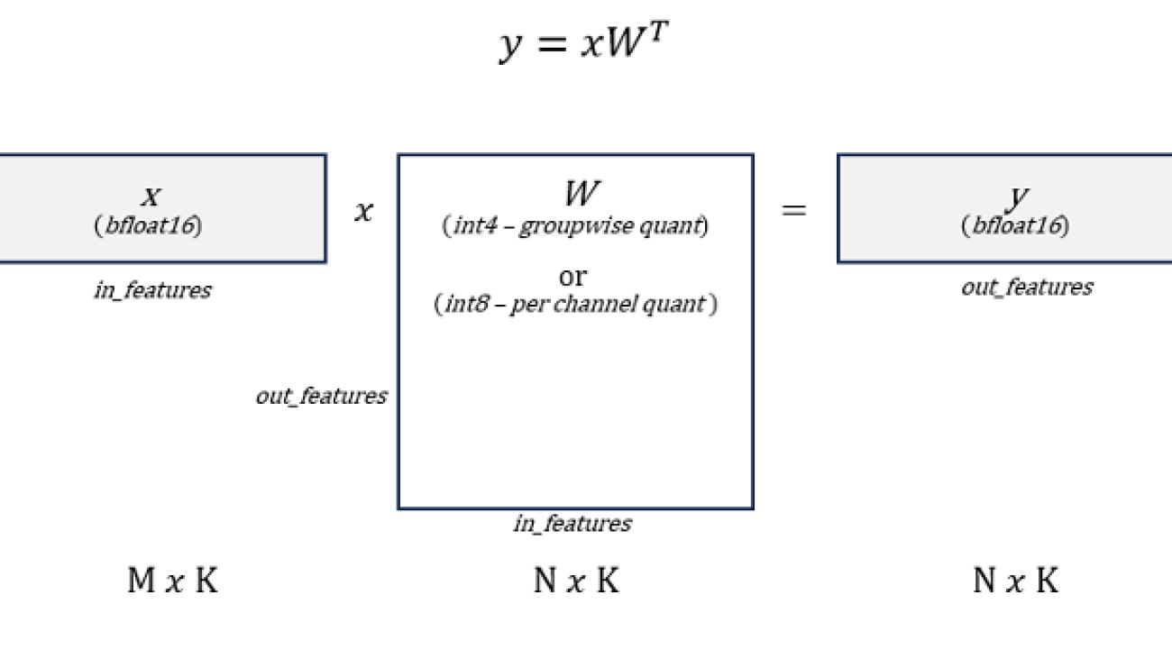
Weight-only quantization (WOQ) is a trade-off between the performance and the accuracy since the bottleneck of the auto-regressive decoding phase in text generation is the memory bandwidth of loading weights and generally WOQ could lead to better accuracy compared to traditional quantization approach such as W8A8. GPTFast supports two types of WOQs: W8A16 and W4A16. To be specific, activations are stored in BFloat16 and model weights could be quantized to int8 and int4, as shown in Figure 1.
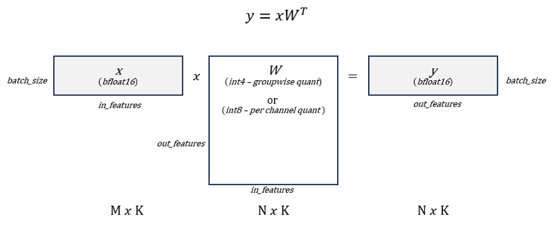
Figure 1. Weight-only Quantization Pattern. Source: Mingfei Ma, Intel
-
Weight Prepacking & Micro Kernel Design.
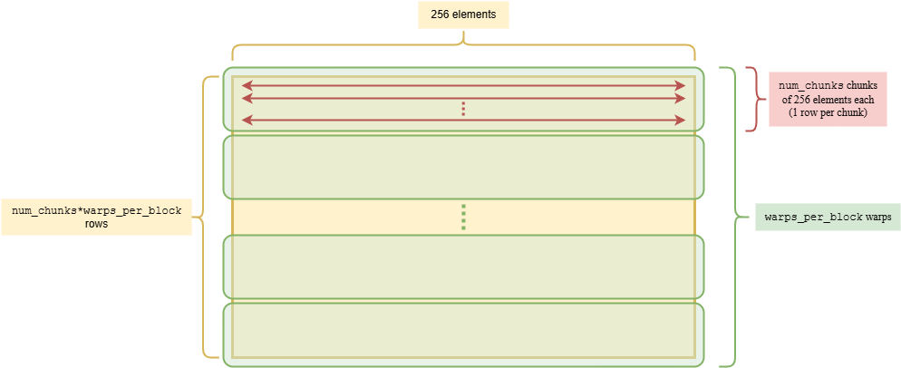
To maximize throughput, GPTFast allows model weights to be prepacked into hardware-specific layouts on int4 using internal PyTorch ATen APIs. Inspired by Llama.cpp, we prepacked the model weights from [N, K] to [N/kNTileSize, K, kNTileSize/2], with kNTileSize set to 64 on avx512. First, the model weights are blocked along the N dimension, then the two innermost dimensions are transposed. To minimize de-quantization overhead in kernel computation, we shuffle the 64 data elements on the same row in an interleaved pattern, packing Lane2 & Lane0 together and Lane3 & Lane1 together, as illustrated in Figure 2.
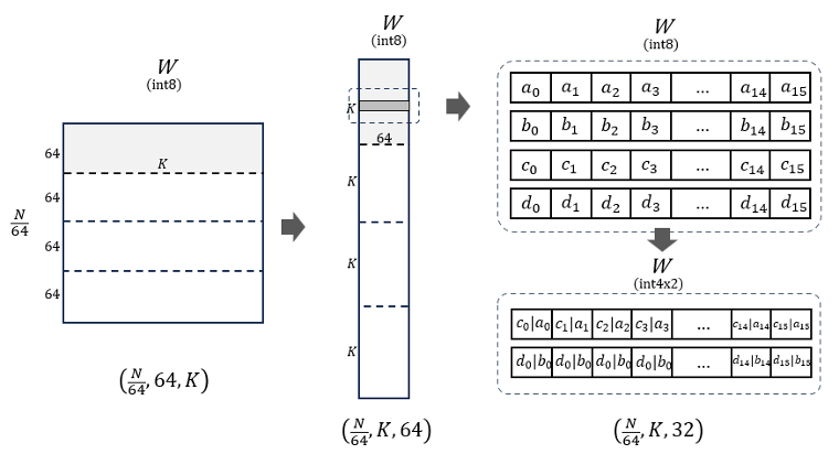
Figure 2. Weight Prepacking on Int4. Source: Mingfei Ma, Intel
During the generation phase, the torch.nn.Linear module will be lowered to be computed with high-performance kernels inside PyTorch ATen, where the quantized weights will be de-quantized first and then accumulated with fused multiply-add (FMA) at the register level, as shown in Figure 3.
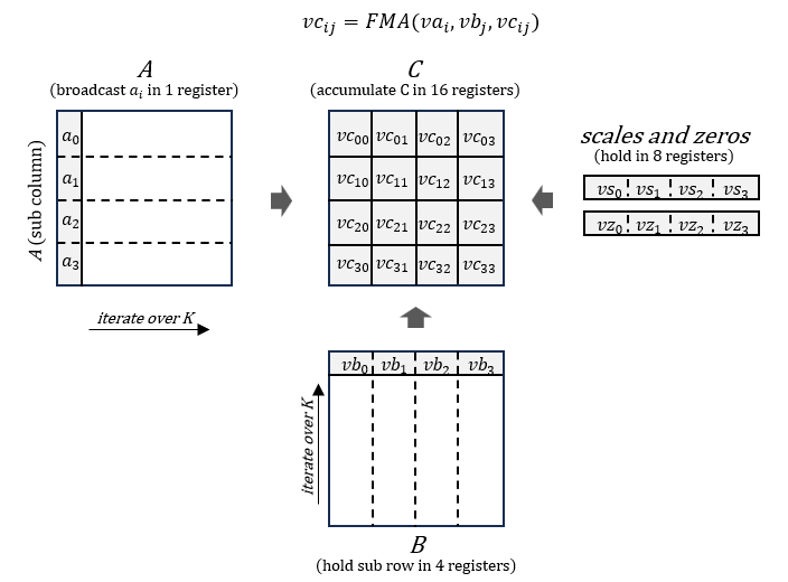
Figure 3. Micro Kernel Design. Source: Mingfei Ma, Intel
Segment Anything Fast
Segment Anything Fast offers a simple and efficient PyTorch native acceleration for the Segment Anything Model (SAM) , which is a zero-shot vision model for generating promptable image masks. The following are optimization strategies used to boost performance on PyTorch CPU:
-
BFloat16
Bfloat16 is a commonly used half-precision type. Through less precision per parameter and activations, we can save significant time and memory in computation.
-
Torch.compile
torch.compile is a PyTorch function introduced since PyTorch 2.0 that aims to solve the problem of accurate graph capturing in PyTorch and ultimately enable developers to run their PyTorch programs faster.
-
Scaled Dot Product Attention (SDPA)
Scaled Dot-Product Attention (SDPA) is a crucial mechanism in transformer models. PyTorch offers a fused implementation that significantly outperforms a naive approaches. For Segment Anything Fast, we convert the attention mask from bfloat16 to float32 in a block-wise manner. This method not only reduces peak memory usage, making it ideal for systems with limited memory resources, but also enhances performance.
Diffusion Fast
Diffusion Fast offers a simple and efficient PyTorch native acceleration for text-to-image diffusion models. The following are optimization strategies used to boost performance on PyTorch CPU:
-
BFloat16
Bfloat16 is a commonly used half-precision type. Through less precision per parameter and activations, we can save significant time and memory in computation.
-
Torch.compile
torch.compile is a PyTorch function introduced since PyTorch 2.0 that aims to solve the problem of accurate graph capturing in PyTorch and ultimately enable software engineers to run their PyTorch programs faster.
-
Scaled Dot Product Attention (SDPA)
SDPA is a key mechanism used in transformer models, PyTorch provides a fused implementation to show large performance benefits over a naive implementation.
Model Usage on Native PyTorch CPU
GPTFast
To launch WOQ in GPTFast, first quantize the model weights. For example, to quantize with int4 and group size of 32:
python quantize.py --checkpoint_path checkpoints/$MODEL_REPO/model.pth --mode int4 –group size 32
Then run generation by passing the int4 checkpoint to generate.py
python generate.py --checkpoint_path checkpoints/$MODEL_REPO/model_int4.g32.pth --compile --device $DEVICE
To use CPU backend in GPTFast, simply switch DEVICE variable from cuda to CPU.
Segment Anything Fast
cd experiments

export SEGMENT_ANYTHING_FAST_USE_FLASH_4=0

python run_experiments.py 16 vit_b <pytorch_github> <segment-anything_github> <path_to_experiments_data> --run-experiments --num-workers 32 --device cpu

python run_experiments.py 16 vit_h <pytorch_github> <segment-anything_github> <path_to_experiments_data> --run-experiments --num-workers 32 --device cpu
Diffusion Fast
python run_benchmark.py --compile_unet --compile_vae --device=cpu
Performance Evaluation
GPTFast
We ran llama-2-7b-chat model based on test branch and the above hardware configuration on PyTorch. After applying the following steps, we saw a 3.8x boost compared to the baseline in eager mode:
- Use
torch.compileto automatically fuse elementwise operators. - Reduce memory footprint with WOQ-int8.
- Further reduce memory footprint with WOQ-int4.
- Use AVX512 which enables faster de-quant in micro kernels.
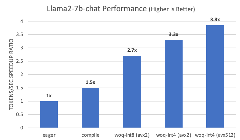
Figure 4. GPTFast Performance speedup in Llama2-7b-chat
Segment Anything Fast
We ran Segment Anything Fast on the above hardware configuration on PyTorch and achieved a performance speedup of BFloat16 with torch.compile and SDPA compared with FP32 as shown in Figure 5. The speedup ratio against FP32 can achieve 2.91x in vit_b, and 3.95x in vit_h.
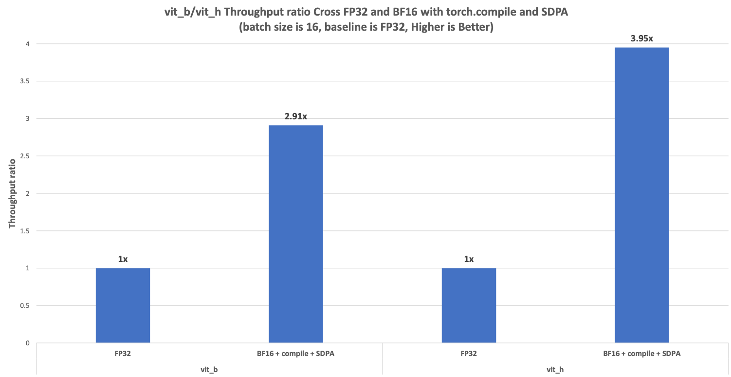
Figure 5. Segment Anything Fast Performance speedup in vit_b/vit_h
Diffusion Fast
We ran Diffusion Fast on the above hardware configuration on PyTorch and achieved a performance speedup of BFloat16 with torch.compile and SDPA compared with FP32 as shown in Figure 6. The speedup ratio against FP32 can achieve 3.91x in Stable Diffusion XL (SDXL).
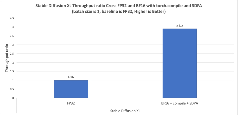
Figure 6. Diffusion Fast Performance speedup in Stable Diffusion XL
Conclusion and Future Work
In this blog, we introduced software optimizations for weight-only quantization, torch.compile, and SDPA, demonstrating how we can accelerate text generation with native PyTorch on CPU. Further improvements are expected with the support of the AMX-BF16 instruction set and the optimization of dynamic int8 quantization using torchao on CPU. We will continue to extend our software optimization efforts to a broader scope.
Acknowledgments
The results presented in this blog are a joint effort between Meta and the Intel PyTorch Team. Special thanks to Michael Gschwind from Meta who spent precious time providing substantial assistance. Together we took one more step on the path to improve the PyTorch CPU ecosystem.
Related Blogs
Part 1: How to accelerate Segment Anything over 8x with Segment Anything Fast.
Part 2: How to accelerate Llama-7B by almost 10x with help of GPTFast.
Part 3: How to accelerate text-to-image diffusion models up to 3x with Diffusion Fast.
Part 4: How to speed up FAIR’s Seamless M4T-v2 model by 2.7x.
Product and Performance Information
Figure 4: Intel Xeon Scalable Processors: Measurement on 4th Gen Intel Xeon Scalable processor using: 2x Intel(R) Xeon(R) Platinum 8480+, 56cores, HT On, Turbo On, NUMA 2, Integrated Accelerators Available [used]: DLB 2 [0], DSA 2 [0], IAA 2 [0], QAT 2 [0], Total Memory 512GB (16x32GB DDR5 4800 MT/s [4800 MT/s]), BIOS 3B07.TEL2P1, microcode 0x2b000590, Samsung SSD 970 EVO Plus 2TB, CentOS Stream 9, 5.14.0-437.el9.x86_64, run single socket (1 instances in total with: 56 cores per instance, Batch Size 1 per instance), Models run with PyTorch 2.5 wheel. Test by Intel on 10/15/24.
Figure 5: Intel Xeon Scalable Processors: Measurement on 4th Gen Intel Xeon Scalable processor using: 2x Intel(R) Xeon(R) Platinum 8480+, 56cores, HT On, Turbo On, NUMA 2, Integrated Accelerators Available [used]: DLB 2 [0], DSA 2 [0], IAA 2 [0], QAT 2 [0], Total Memory 512GB (16x32GB DDR5 4800 MT/s [4800 MT/s]), BIOS 3B07.TEL2P1, microcode 0x2b000590, Samsung SSD 970 EVO Plus 2TB, CentOS Stream 9, 5.14.0-437.el9.x86_64, run single socket (1 instances in total with: 56 cores per instance, Batch Size 16 per instance), Models run with PyTorch 2.5 wheel. Test by Intel on 10/15/24.
Figure 6: Intel Xeon Scalable Processors: Measurement on 4th Gen Intel Xeon Scalable processor using: 2x Intel(R) Xeon(R) Platinum 8480+, 56cores, HT On, Turbo On, NUMA 2, Integrated Accelerators Available [used]: DLB 2 [0], DSA 2 [0], IAA 2 [0], QAT 2 [0], Total Memory 512GB (16x32GB DDR5 4800 MT/s [4800 MT/s]), BIOS 3B07.TEL2P1, microcode 0x2b000590, Samsung SSD 970 EVO Plus 2TB, CentOS Stream 9, 5.14.0-437.el9.x86_64, run single socket (1 instances in total with: 56 cores per instance, Batch Size 1 per instance), Models run with PyTorch 2.5 wheel. Test by Intel on 10/15/24.
Notices and Disclaimers
Performance varies by use, configuration and other factors. Learn more on the Performance Index site. Performance results are based on testing as of dates shown in configurations and may not reflect all publicly available updates. See backup for configuration details. No product or component can be absolutely secure. Your costs and results may vary. Intel technologies may require enabled hardware, software or service activation.
Intel Corporation. Intel, the Intel logo, and other Intel marks are trademarks of Intel Corporation or its subsidiaries. Other names and brands may be claimed as the property of others.
AI disclaimer:
AI features may require software purchase, subscription or enablement by a software or platform provider, or may have specific configuration or compatibility requirements. Details at www.intel.com/AIPC. Results may vary.